The role of non-conservative scattering forces and damping on Brownian particles in optical traps
Matthieu Mangeat, Yacine Amarouchene, Yann Louyer, Thomas Gu\'erin and, David S. Dean

TL;DR
This paper investigates how non-conservative forces and damping influence the steady state and spectral properties of Brownian particles in optical traps, revealing strong signatures especially in underdamped regimes.
Contribution
It provides a comprehensive theoretical analysis of non-conservative forces on trapped particles, including probability distributions, phase space currents, and spectral densities across all dynamical regimes.
Findings
Non-conservative forces significantly alter steady state distributions.
Spectral density shows strong signatures of non-conservative forces in underdamped regimes.
Perturbative expressions are derived for all dynamical regimes.
Abstract
We consider a model of a particle trapped in a harmonic optical trap but with the addition of a non-conservative radiation induced force. This model is known to correctly describe experimentally observed trapped particle statistics for a wide range of physical parameters such as temperature and pressure. We theoretically analyse the effect of non-conservative force on the underlying steady state distribution as well as the power spectrum for the particle position. We compute perturbatively the probability distribution of the resulting non-equilibrium steady states for all dynamical regimes, underdamped through to overdamped and give expressions for the associated currents in phase space (position and velocity). We also give the spectral density of the trapped particle's position in all dynamical regimes and for any value of the non-conservative force. Signatures of the presence…
Click any figure to enlarge with its caption.
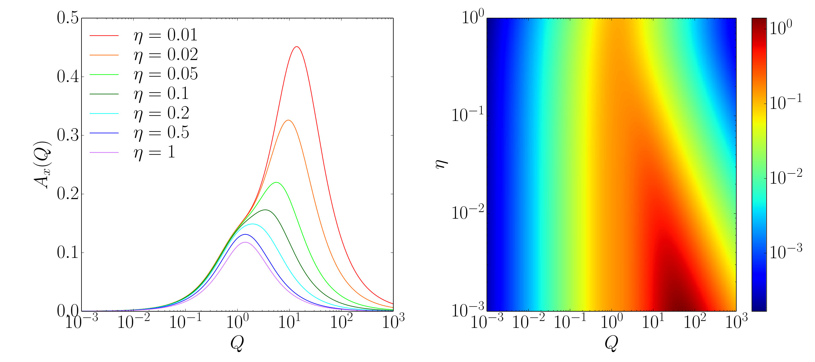 Figure 1
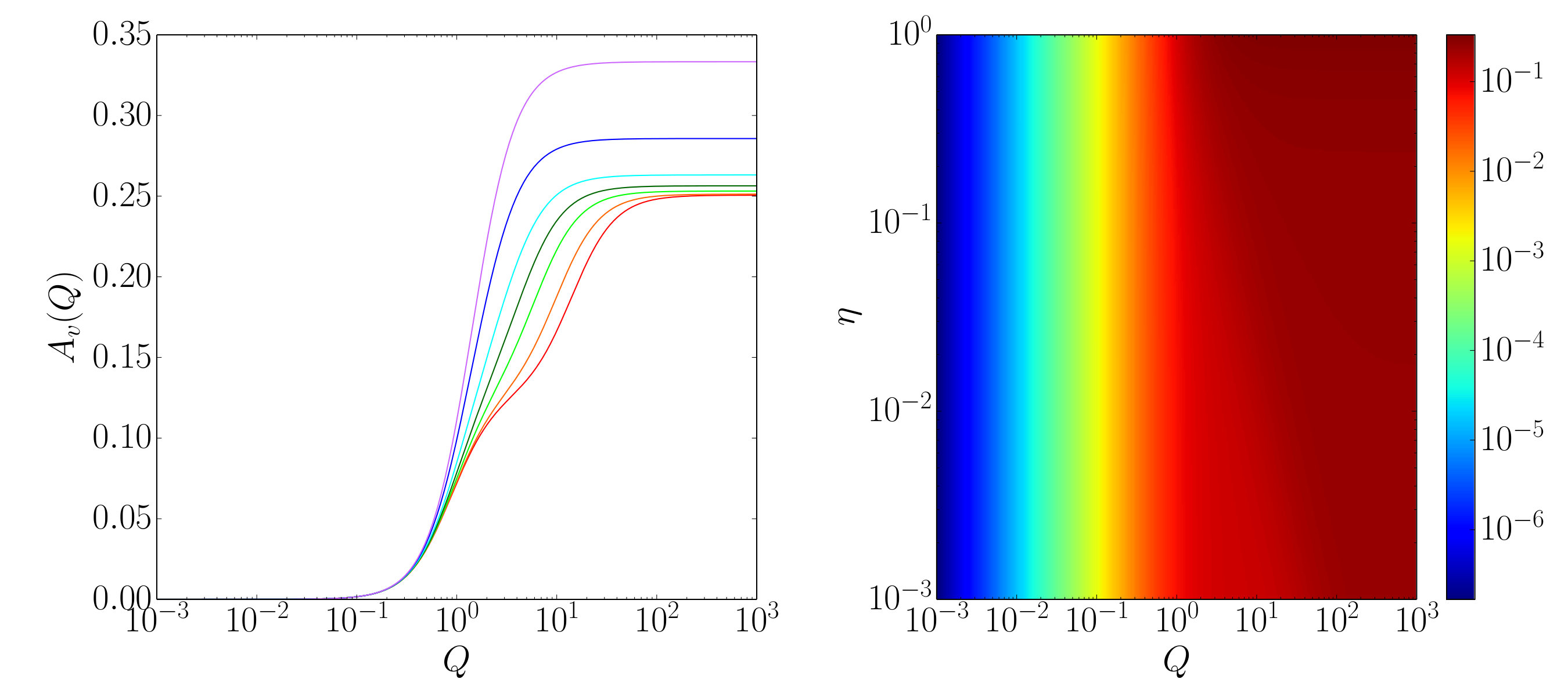 Figure 2
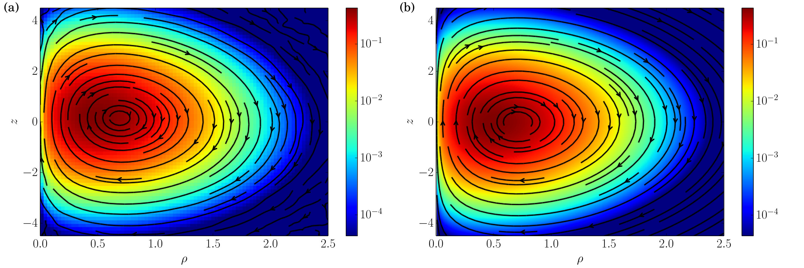 Figure 3
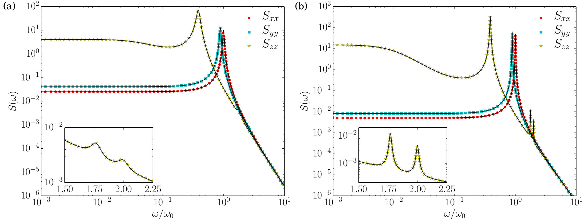 Figure 4
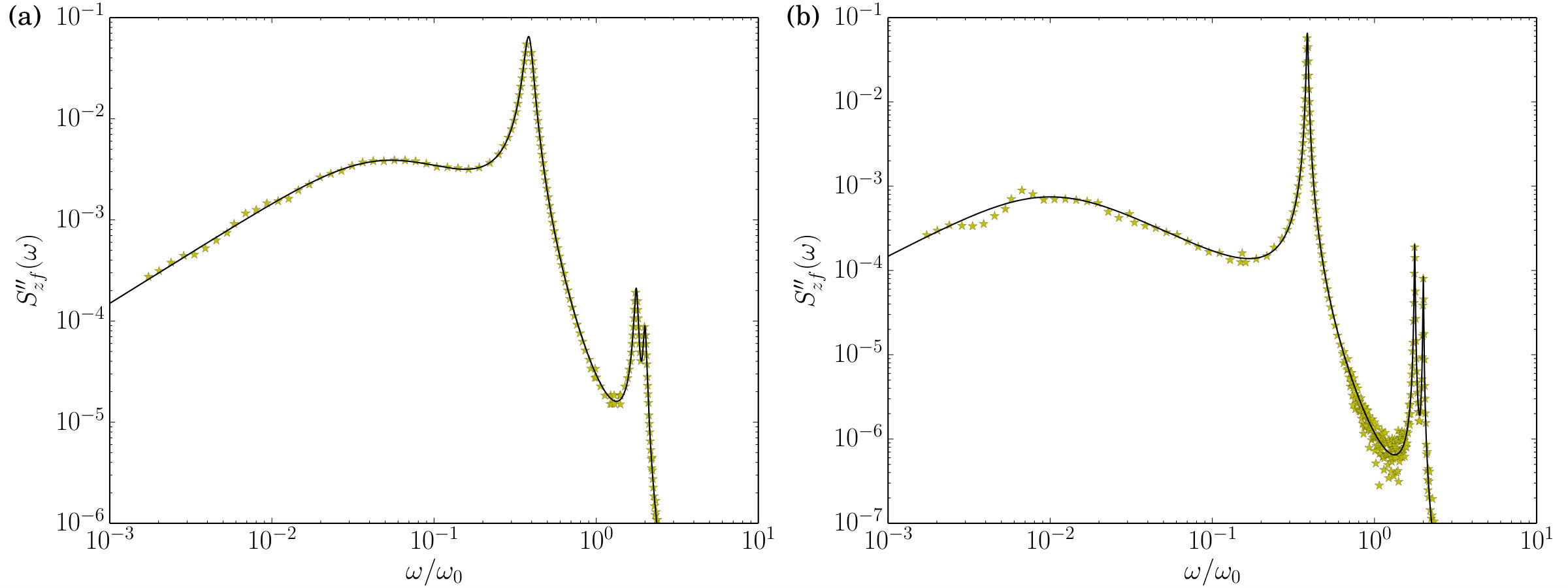 Figure 5
Peer Reviews
No public reviews on file for this paper yet. If you reviewed it on a platform where reviews are public (OpenReview, ICLR, NeurIPS, ICML), you can paste yours below so the community can read it here.
Videos
No videos yet. Explain this paper in a talk, walkthrough, or lecture? Add one.
The role of non-conservative scattering forces and damping on Brownian particles in optical traps
Matthieu Mangeat, Yacine Amarouchene, Yann Louyer, Thomas Guérin and David S. Dean
Univ. Bordeaux, CNRS, LOMA, UMR 5798, F-33400 Talence, France
Abstract
We consider a model of a particle trapped in a harmonic optical trap but with the addition of a non-conservative radiation induced force. This model is known to correctly describe experimentally observed trapped particle statistics for a wide range of physical parameters such as temperature and pressure. We theoretically analyse the effect of non-conservative force on the underlying steady state distribution as well as the power spectrum for the particle position. We compute perturbatively the probability distribution of the resulting non-equilibrium steady states for all dynamical regimes, underdamped through to overdamped and give expressions for the associated currents in phase space (position and velocity). We also give the spectral density of the trapped particle’s position in all dynamical regimes and for any value of the non-conservative force. Signatures of the presence non-conservative forces are shown to be particularly strong for in the underdamped regime at low frequencies.
I Introduction
The seminal work of Ashkin in the 1970s instigated the development of optical traps ash . Optical traps or tweezers are an invaluable tool for studying statistical mechanics, both in an out of equilibrium, at the level of single particles. Moving the center of the optical trap allows one to measure very small forces in a wide range of systems, including colloids colloid , biological systems (for instance viruses, proteins and biopolymers) bio , as well as dielectric and metallic nano-particles nano . The same kind of perturbation can be used to analyze non-equilibrium processes, for instance optical tweezers have been used to demonstrate various non-equilibrium fluctuation theorems fluct . However in such studies the optical trap does not simply furnish a simple potential, optical scattering forces actually generate a non-conservative component to the overall force exerted by the trap. Because of the presence of these scattering forces, even static optical traps represent non-equilibrium systems as the particles trapped within them are driven by the non-conservative forces and thus are not described by a Gibbs-Boltzmann probability distribution. For instance, it has been demonstrated grier2008 ; grier2009 ; grier2010 ; grier2015 both theoretically and experimentally that scattering forces induce non-equilibrium currents, so called Brownian vortices, for trapped overdamped Brownian particles. At atmospheric pressures and near room temperatures, the underlying dynamics of a trapped particle can be taken to be overdamped Brownian. However optical traps operated at low pressure can probe dynamics where inertial effects become important and cross over to the underdamped regime. Clearly the current state of the art of the theory has to be modified to take into account the effects of inertia and this is the goal of this paper. Using the model of a Gaussian optical trap in the presence of a simplified non-conservative force we examine the impact of inertial effects across the whole regime between overdamped and underdamped Brownian motion.
First a general theory for the probability distribution of the perturbed steady state due to a small non-conservative force is developed for general damped Brownian dynamics. The modification of the steady state probability distribution function for the full phase space in the optical model of grier2015 is found and the resulting marginal probability distributions for the particle position and velocity is computed. We demonstrate that the Brownian vortices found in the current of the particle position persists and remains geometrically the same as that found in grier2015 . However the amplitude of the vortices depends on the damping parameters, we will show that this damping parameter can be tuned in order to optimize the non-equilibrium current. In addition, we show that there is a non-equilibrium current in the space of velocities, the vortex here turns out to be remarkably similar to the vortex in position space.
For the optical trap model of grier2015 we also compute the spectral density of the particle position for general damping. Our result recovers the computation of laporta2011 for overdamped Brownian motion and generalizes it to all damping regimes. Here we see that the non-conservative force generates very strong changes in the spectral density at low frequencies and that the amplitude of the low frequency spectral density can be tuned by varying the friction coefficient and that there is a critical value of where it is minimized. Finally, we also derive a function correlation which is a signal of the breaking of time reversal symmetry due to the non-conservative optical scattering force.
Some of the results derived in this paper are used in a accompanying letter, where the role of inertia in the presence of non-conservative forces is demonstrated in the experimental context letter . In this paper we concentrate on the presence of a nonconservative force in addition to a purely harmonic trap. This simplified model allows the derivation of a large number of analytical results. However, to fully explain the results of letter , where small anharmonicities can give rise to large effects in the underdamped regime due to near resonance phenomena, quartic terms in the potential must be considered to fully reproduce the experimental results. However the results derived here can be adapted to the experimental context by using effective harmonic parameters describing the nonlinear system Renz1 . This therefore yields an analytic theory sufficient to completely describe the experiments and fully non-linear numerical simulations letter .
II Modeling particles in optical traps
II.1 Langevin Dynamics
In this section we first discuss the underlying Langevin dynamics used to model the trapped particle. We then discuss the underlying model for trapping, aimed at experts in non-equilibrium statistical mechanics who are perhaps not familiar with the physics of optical trapping.
In this paper we will consider the dynamics of Brownian particles in an optical trap. If denotes the particle position, the underlying Langevin equation is
[TABLE]
where is the particle mass, the friction coefficient and is a time independent force generated by the optical trap. The noise term is assumed to have Gaussian white noise correlations in time, this noise has zero mean and correlation function
[TABLE]
in the amplitude term is the temperature measured in units where . When the trap is applied in a gas phase the friction coefficient can be significantly modified and one can go from the underdamped to overdamped regimes with the same experimental set up if one can control the pressure in the trapping cell.
A semi-phenomenological relationship the friction coefficient in air as a function of the pressure is given by beresnev1990 ; Li2013
[TABLE]
where in the first, Stokes drag-like, term is the radius of the particle and the viscosity coefficient of air at atmospheric pressure. In addition, is the Knudsen number, accounting from the deviation from continuum behavior, where is the mean free path of air molecules and is given by , where is the applied pressure in the trap and is the atmospheric pressure. Finally . We thus see that the value of the friction coefficient can be tuned by modifying the pressure of the trap.
II.2 Model of the optical trap
In the experiment described in the accompanying paper letter , the wave length of the laser is , while the radius of the trapped (fused silica) particle is . As , we are in the Rayleigh regime, where the particle can be treated as a point dipole.
Here for completeness we review the model of the optical trap used in quid2013 as well as reviewing the underlying physics giving rise to both conservative and non-conservative forces in the dipole approximation hecht2006 . The Lorentz force acting on an electric dipole is given by
[TABLE]
The response of the dipole to the applied electric field is taken to be linear
[TABLE]
For a mono-chromatic electromagnetic field of angular frequency polarized in the direction we can write
[TABLE]
where denotes the unit vector in the direction and is the phase. Using the Maxwell equation we can write
[TABLE]
Using linear response we can write
[TABLE]
so is the polarizability at frequency and and denote the real (dispersive) and imaginary (dissipative) parts respectively. Now evaluating the force and replacing the terms and by their temporal average and cross terms and by their temporal average [math] we obtain
[TABLE]
where is the field intensity. The first term above is clearly a conservative force generated by the potential
[TABLE]
The second term contains in general a non-conservative component. Its underlying origin comes from the interaction of the magnetic field with the rate of change of the dipole moment.
The electric field produced by the laser is approximated by the Gaussian form
[TABLE]
where the field is polarized in the direction and for we have
[TABLE]
is the dependent beam radius. The phase is given by
[TABLE]
where is the wave vector. The parameter is the Rayleigh range and is normally used as a fitting parameter, however it is predicted to be given by . Finally, the particle is assumed to be spherical and the polarizability is taken to be hecht2006
[TABLE]
where is the zero-frequency polarizability given by
[TABLE]
and is the dielectric constant of the vaccum while is the relative dielectric constant of the particle. The form of the electric field given by Eq. (11) arises from the paraxial approximation to Maxwell’s equation for the electric field in the vacuum, and in this case the corresponding Helmholtz equation. The paraxial approximation assumes that for the whole electric field function denoted by (polarized in the direction ) one has that . Inspection of Eqs. (11) and (13) show that the paraxial approximation is valid when , and one can expand the force perturbatively for small when . The first inequality implies that we must have .
In the accompanying letter letter the laser waist parameters are estimated in the high pressure regime where both the effects of trap nonlinearities and the scattering forces are weak. It is found that , and (in the notation of letter ) and so we must have . In addition, one may also Taylor expand the forces when and are small, experimental results show that these two values are both of the order of , so while non-linear effects are weak they are not completely negligible.
Under the above assumptions, to lowest order, the potential part of the force is generated by a quadratic potential
[TABLE]
with spring constants given by , and .
The phase factor is given, expanding to first and next order of the particle displacement, by
[TABLE]
As mentioned above, the term is often treated as a fitting parameter as the solution Eq. (11) is an approximate solution. However an alternative physical approach is to insist that the approximated solution obeys Maxwell’s equations exactly near the center of the trap. Expanding the solution for small , and up to cubic order we find that
[TABLE]
Now using the Helmholtz equation near the origin we find the equation, coming from the real term,
[TABLE]
giving an exact relation between and the two waists and in terms of the wave vector . In the case where and when (so we assume that the paraxial approximation is valid) we obtain the standard formula . However this formula is only valid if . Taking the root of Eq. (19) compatible with the standard formula we find
[TABLE]
or in terms of the wavelength we have
[TABLE]
Using this to determine , with the values of and determined above yields , which is different from the fully fitted value of by about . This estimate thus provides a useful starting point to determine the trap parameters in the fitting procedure.
The scattering part of the force is given to leading, quadratic, order by
[TABLE]
which can be written in terms of the spring constant as
[TABLE]
which gives
[TABLE]
The lowest order approximation that takes into account both conservative/potential and scattering forces is thus the expressions for () and (). The next order corrections are terms to coming from anharmonic contributions.
Using the form Eq. (11) in the Helmholtz equation without making any approximations yields
[TABLE]
The real and imaginary parts of the above give two equations. The scattering force is given by
[TABLE]
and taking the divergence of this yields
[TABLE]
from Eq. (25). However the result Eq. (24) gives . In the limit , where the paraxial approximation becomes exact we find that this term is zero, but in general it is not. This actually mean that the very last term in Eq. (24) should not be there. This can be regarded as being due to an error in the phase term.
Taking this into account we can naturally divide the scattering force into two components
[TABLE]
where
[TABLE]
and
[TABLE]
For the values of obtained here the dominant scattering force is , however as scales as when just the harmonic confinement is taken into account it is not evident that the last term in the direction can be neglected. However we find that numerically this turns out to be the case.
III Perturbative calculation of the non-equilibrium steady state probability density function and current
In the standard paradigm of statistical physics, Brownian particles are subjected to forces generated by potentials and this means that the underlying steady state distribution is given by the Gibbs-Boltzmann distribution. The crucial point here is that the steady state in the presence of a nonconservative force has an associated current. We note that Brownian particles subject to linear potentials in unbounded systems also have currents, however because the system is unbounded the probability distribution spreads with time and can be associated with effective transport coefficients dea2007 . However in periodic systems the particle position modulo the period of the system does have a steady state which carries a current, and this system can be analysed for overdamped Brownian particles reim2001 . In general very few results exist on the steady states of systems with nonconservative forces or in the presence of driving, even for trapped mono-particle systems where only one body forces are present. Here we will resort to the use of perturbation theory, which can be justified when the nonconservative component of the force is weak in comparison to the conservative component. Indeed, perturbation theory was the approach employed in grier2015 to analyse a trapped overdamped Brownian particle.
We will consider systems which are driven by underlying white noise, and thus include both underdamped and overdamped Brownian motion. The probability distribution of the particle’s position in phase space is thus described by the Fokker-Planck equation
[TABLE]
where denote the phase-space coordinates and is the forward Fokker-Planck operator. Before perturbation by a non-conservative force we assume that the system obeys detailed balance and has an underlying Gibbs-Boltzmann distribution denoted by , obeying
[TABLE]
Now we consider what happens when the system is perturbed by an additional force which is in terms of the Fokker-Planck operator denoted by the perturbation . The question we address is what is the new steady state distribution defined by
[TABLE]
To first order in perturbation theory we write where is given by
[TABLE]
This now has the formal solution
[TABLE]
Here is the pseudo-Green’s function for the operator as the solution must obey the normalization
[TABLE]
The transition probability can formally be written as
[TABLE]
and the pseudo-Green’s function thus as
[TABLE]
This yields
[TABLE]
Now using the time reversal symmetry of the equilibrium state
[TABLE]
where ∗ indicates time reversal of the coordinates, this means that coordinates with an odd number of temporal derivatives change sign. Taking we see that time reversal symmetry also implies that . For overdamped Brownian particles this has no effect as the position vector obeys . However if represents the position and velocity we have . We thus find
[TABLE]
If the stochastic process represented by the Fokker-Planck equation is denoted by and we use the notation
[TABLE]
i.e. the average value of at time given that , and
[TABLE]
the equilibrium value of . We thus change the integration variable to write
[TABLE]
where we have used . This then yields
[TABLE]
The change in the equilibrium distribution at the point in phase space is thus given by a Kubo-type formula kubo . This result is general and applies to any system described by a Fokker-Planck equation.
III.1 Overdamped Brownian motion
Here we consider a process characterized solely by the position , that is to say the overdamped regimes. Here we assume that the unperturbed Fokker Planck operator, defined via its action on a test function , is given by
[TABLE]
i.e. it describes a particle with diffusivity in a potential at temperature (where for convenience we use units where , the results for measured in Kelvin are thus obtained by replacing by in all the formulas which follow) and .
Here the steady state is given by the Gibbs-Boltzmann equilibrium distribution
[TABLE]
The perturbation of the Fokker-Planck operator due to the presence of an extra force is given by
[TABLE]
From this we find
[TABLE]
This now gives
[TABLE]
The case where the force is derived from a potential, , should of course be simple as we know the new equilibrium measure should be
[TABLE]
and for small should find
[TABLE]
It is illuminating, as well as a useful check, to obtain this from the general formalism derived previously. To do this, we use the following result of stochastic calculus osk for an arbitrary function :
[TABLE]
Using this and the relation in Eq. (50) now gives
[TABLE]
Clearly we have
[TABLE]
and also we have by definition that
[TABLE]
The time integral in Eq. (54) can now be simply carried out to yield
[TABLE]
in agreement with Eq. (52).
In general the perturbing force can be decomposed into a conservative and nonconservative part via the Helmholtz decomposition where one writes
[TABLE]
where is determined from the equation
[TABLE]
and the remaining term can be similarly evaluated to write
[TABLE]
where the nonconservative part of the force is given by
[TABLE]
however, the solution for must be chosen so that . Using this decomposition then yields
[TABLE]
The modification of the steady state probability density function by the non-conservative force is thus seen to be related to the work done by the non-conservative force in the direction of the original potential . This formula is not particularly illuminating from a physical point of view for overdamped Brownian motion, when we study the case of general damping we will find a much more explicit interpretation.
III.1.1 Application to a model for an optical trap
Here we study the model proposed by Grier et al grier2015 , where
[TABLE]
so this represents an anisotropic harmonic trap unless . We have seen that the potential part of the scattering force in Eq. (16) in general also has as the difference between and is numerically small we carry out the analysis for this case to simplify the notation and the following analysis. In grier2015 the nonconservative component of the force generated by the optical trap is taken to be
[TABLE]
is proportional to the waist (we use the same notation as grier2015 for ease of comparison). The part of the scattering force used is thus , expressed in Eq. (29) which is that which is numerically the most important. However the nature of our perturbative computation means that the corrections to from each component of the non-conservative force is additive, and so we can simply compute the perturbations due to each component and then sum them. The perturbing parameter is dimensionless and we will compute the modified steady state probability density function to first order in .
The decomposition of the perturbation in terms of a conservative and nonconservative contribution now yields the potential
[TABLE]
and the nonconservative component of the force
[TABLE]
Using this we find
[TABLE]
The evaluations of the expectation values required to compute the renormalization of the steady state probability distribution can be carried out by explicitly solving the Langevin equation for the unperturbed process, the corresponding equations are
[TABLE]
where , and are independent Gaussian white noises. The above equations can be solved in terms of the particle positions at , denoted by , and to give
[TABLE]
Using these solutions we find
[TABLE]
and we also see that
[TABLE]
Putting all this together (and noting that ) we obtain
[TABLE]
where is interpreted as the renormalization of the trapping potential. This agrees with the result found in grier2015 for the same trapping potential and nonconservative perturbation considered here.
III.1.2 Alternative formulation for overdamped particles
The probabilistically based solution for the perturbed steady state distribution gives us an interpretation of the perturbation of the steady state in terms of work done by the perturbing forces. However in the case where the unperturbed solution is Gaussian we see that the solution is particularly simple, the solution having a polynomial form for a polynomial perturbing force. Given the structure of the solution found we make the same ansatz as in grier2015
[TABLE]
this yields
[TABLE]
For the case studied above as defined by the potential in Eq. (63) and the force in Eq. (64) we find
[TABLE]
Inspection of the probabilistic representation of the solution, and from the symmetry of the problem in the plane, now tells us that the solution must have the form
[TABLE]
this yields
[TABLE]
and comparing the coefficients of the polynomials now gives
[TABLE]
in agreement with the earlier calculation leading to Eq. (76) and thus the result given in grier2015 .
Here we also consider the perturbation to a force of type derived in Eq. (30) which we write as
[TABLE]
as it has no potential part. Here we find
[TABLE]
where the ′ on denotes that it is the form of for the perturbation . Here we see that the solution must be of the form
[TABLE]
This gives
[TABLE]
and thus
[TABLE]
This therefore gives a contribution to the steady state distribution
[TABLE]
III.2 Underdamped Brownian particles
Here the phase space corresponds to where and denote respectively the particle position and its velocity. Here the Fokker-Planck operator is given by
[TABLE]
where is the friction coefficient, is the particle mass, and is the total force on the particle which is assumed to depend only on the position . For the unperturbed system we take . The equilibrium distribution is then given by
[TABLE]
In the perturbed system we denote the additional force simply by . This yields
[TABLE]
and thus
[TABLE]
where we have used . The result in Eq. (95) immediately gives us a physical interpretation of the modification of the steady state probability density function. We see that
[TABLE]
where is the total work done, after a very long time , by the non-conservative force on a particle started at the posiiton but and with initial velocity , whereas is the total work done by the non-conservative force, at the same late time , for a particle whose initial velocity and position are taken from the unperturbed equilibrium probability density function. Both of these total works diverge as but their difference is constant. When the perturbing force is purely conservative, i.e. we immediately obtain, much more transparently that in the Brownian case,
[TABLE]
and as we find, using the same arguments as for the overdamped case
[TABLE]
thus recovering the corresponding modified Gibbs-Boltzmann distribution.
III.3 Application to under generally damped particles in optical trap model
In principle, for a harmonic trap all the average values in Eq. (95) can be computed. However, as for the overdamped case, the form of the solution suggests writing
[TABLE]
This then yields
[TABLE]
There is a distinct advantage, at least for complex perturbations by non-conservative forces, of using this algebraic formulation as opposed to the probabilistic representation. However the probabilistic representation allows one to predict the polynomial form of and only the coefficients of this polynomial need be determined after substituting the correct form of into Eq. (100). This is because in the expression we can see explicitly what terms in the initial position and velocity must arise by inspecting the form of given in Eq. (64).
From the symmetry in the plane, the solution of Eq. (100) must have the form
[TABLE]
After simplification, the coefficients are given by
[TABLE]
where . Using these expressions we have thus computed the perturbed probability density function in the full phase space. However the final expressions are rather unwieldy, we will therefore give explicit expressions for the marginal probability density functions of and then .
Denoting the marginal steady state probability density function for the position by , we find from Eq. (93)-(101)
[TABLE]
where . In the underdamped limit , we find thus
[TABLE]
and in the overdamped limit , we recover (for a third time) the result of grier2015 Eq. (76).
Using the modified probability density function in Eq. (110) can study various moments of the particle position. The average value of the height of the particle is given by
[TABLE]
while the average velocity in the direction is given by , after some mathematical cancellations which appear remarkable from a mathematical point of view but obvious from the simple physical insight that the particle is trapped! The above result for is thus independent of the details of the dynamics (it is independent of the damping parameters). This surprising result is a consequence of the fact that the average velocity is zero (as obviously must be the case if the particle remains trapped): as the average velocity is zero the mean position along the axis is given by a force balance equation where the friction term is zero and, as the average thermal force and acceleration are zero, the average force balance equation depend only on the external forces acting on the particle and is thus independent of the damping parameters.
Here we introduce the underlying frequency of the harmonic part of the trap and the damping rate . The quality factor is defined as , it quantifies the degree of damping in the system, large corresponding to the underdamped regime and small corresponding to the overdamped regime. In terms of these variables, which are often preferred in experimental studies, we find
[TABLE]
Denoting the marignal steady state probability density function for the velocity by , we find from Eq. (93)-(101)
[TABLE]
where and
[TABLE]
is the Maxwell-Boltzmann velocity distribution. The marginal probability distributions for , and however do not change in first order perturbation theory and are thus given by the Maxwell distribution.
In grier2015 the steady state current was computed for an overdamped Brownian particle. Here we have currents in both position and velocity spaces. From Eq. (92), we see that currents and can be read off from
[TABLE]
where
[TABLE]
The effective currents in position space and velocity space , can be found by integrating Eq. (116) over and respectively to obtain the Fokker-Plank equation for the marginal probability distribution in position, and velocity respectively. From this, and using the divergence theorem, the associated currents can be read off as
[TABLE]
In the non-equilibrium steady state, we find that the currents are given, to first order in the perturbation by the nonconservative force as,
[TABLE]
These expressions can then be rewritten in terms of the function to give
[TABLE]
Using the form of derived for the optical trap model we obtain
[TABLE]
where is the radial unit vector in polar coordinates (recall here ). In the limit , we recover the result of grier2015 for the overdamped case
[TABLE]
where is the effective diffusion constant, as defined by the Einstein relation, . In the underdamped limit , we obtain
[TABLE]
Remarkably the geometry of the current field in space is always the same, the damping parameters only appear via an overall space independent amplitude term such that
[TABLE]
where and
[TABLE]
We see above that when and , and thus the amplitude of the non-equilibrium current can be maximized at a given value of when all other physical parameters are fixed, as can be clearly seen in Fig. 1a. We also see that the amplitude increases as decreases, this is to be expected as the trapping in the direction becomes weaker on reducing .
As pointed out in grier2015 , at the point the direction of the current in the direction reverses, the value of is the value where the particles potential energy due to the harmonic trap attains the equilibrium value as predicted by the equipartition of energy. We also see that the current in the direction is positive for and negative for . The current in the radial (polar coordinate) direction is in the direction and its sign is proportional to , thus the current flows away from the origin in the plane when and towards the origin when .
The current in velocity space is given by
[TABLE]
where . In the overdamped limit, , one finds
[TABLE]
and the limit , we find
[TABLE]
Again we see that the geometric structure in phase space is independent of the damping parameters and that the damping parameters only appear in a velocity independent constant amplitude. Remarkably the geometric structure is basically identical to that of the position current if we reverse the direction and make the correspondence . Here the -dependent amplitude of the current is defined such that
[TABLE]
where , and
[TABLE]
Here we find that as , whereas as . This function is monotonically increasing with , as can be seen in Fig. 2a, it reaches a plateau at large . In contrast to the amplitude of the spatial current we see that the amplitude is largest for large values of , i.e. for strong trapping in the direction.
Note that the apparent divergence for is removed due to the presence of terms of next order in , however the point should present some form of resonance in the current. The value is however far from its typical experimental value which is around letter .
III.4 Application to general particles in optical trap model with the force
We want to find satisfying the equation (100) with defined in Eq. (84) instead of . The solution of this equation must have the form
[TABLE]
After simplification, the coefficients are given by
[TABLE]
where . Denoting the marginal steady state probability density function for the position by , we find from Eq. (93) and (135)
[TABLE]
We recover the Eq. (91) taking the limit . Denoting the marginal steady state probability density function for the velocity by , we find from Eq. (93) and (135)
[TABLE]
The effective current in position space is defined as from Eq. (123). Using the expression of from Eq. (135), we get
[TABLE]
The effective current in velocity space is defined from Eq. (124) as
[TABLE]
After some simplifications, we find
[TABLE]
We see that the above results currents induced by the force are remarkably similar to those induced by the non- conservative part of the force of the force . This can in fact be seen much more easily by noting that the nonconservative parts of and are proportional. Indeed, we can write
[TABLE]
where is a potential difference between the two nonconservative forces. This potential term does not contribute to the current at the order if perturbation theory used here, thus explaining the simple relationship between the two currents found here.
III.5 Comparison with numerical simulation
We will now verify the analytical results for the nonequilibrium steady state probability distribution function and the associated currents, presented above, by comparing them with the results of numerical integration of the corresponding Langevin equations which are given by
[TABLE]
Here, , and are independent Gaussian white noises. We consider the system with the following adimensionalized parameters, where and such that
[TABLE]
where is the quality factor, and and . The numerical integration of these equations is carried out using the algorithm of Sivak et al. sivak2014 . The probability density function is estimated using a spatial binning procedure, for boxes of volume , as
[TABLE]
where if , the particle position at time , is in the bin of and is the total number of points in the trajectory. The spatial current is computed from Eq. (119) using the estimator
[TABLE]
where is the measured particle velocity at time .
The numerically obtained value of the steady state probability distribution for the parameters , , , and while the bins are taken with respect to and (where ). The simulation is carried out using for the integration time step and over a total measurement time for a total of different trajectories. We show in Fig 3(a) the estimated steady state distribution as a grey-scale (color online) plot, along with the vector field plot of the current (shown as arrows). In Fig. 3b we see the corresponding quantities predicted by the perturbation theory employed in this paper. The agreement is excellent, as it should be for the small value of used here.
IV Power spectra for underdamped particles in perturbed Harmonic potentials
The computation of the spectral density function for the particle position in the trap model considered here has been carried out in laporta2011 . Here we generalize this calculation to the case of underdamped Brownian particles and show that significant differences arise. We then verify the calculation by comparing it with numerical simulations.
IV.1 Analytical calculation
Here we compute the power function of an underlying harmonic process subjected to a perturbing non-conservative force. The equations of motion for the components of the particle position are again given by Eqs. (152, 153, 154), and in this particular approximation only the steady state distribution of is changed (the positions and are not coupled to the non-conservative force and the process is a slave to the positions slave ). The addition of the perturbation gives a non-zero average value given by
[TABLE]
Due to the linearity of Eq. (154) we can decompose as
[TABLE]
where is the equilibrium fluctuation due to the thermal noise obeying
[TABLE]
and is the fluctuation in due to the fluctuations of the non-conservative force, then obeys
[TABLE]
where
[TABLE]
is the fluctuating part of the non-conservative noise in the direction. Fourier transforming in time then gives
[TABLE]
and
[TABLE]
The power spectrum of the fluctuations is then given by
[TABLE]
where
[TABLE]
is just given by the ordinary equilibrium fluctuation spectrum
[TABLE]
The contribution from the non-conservative force to the power spectrum is
[TABLE]
Defining
[TABLE]
then gives
[TABLE]
To proceed with the computation of we use
[TABLE]
and so the associated connected correlation function is given by
[TABLE]
In terms of the equilibrium spectral function for
[TABLE]
we thus find
[TABLE]
Using this we obtain
[TABLE]
the last line holding when the system is isotropic in the plane.
In order to compute we note that the poles of are given by
[TABLE]
In the underdamped case where the poles can be written as
[TABLE]
where
[TABLE]
In the evaluation of the integral in Eq. (177) the poles that contribute from come from the upper complex plane and thus only contribute. The poles of can be written to be at and thus . Therefore, only the poles contribute from . In terms of these poles we can write
[TABLE]
Evaluating the residues in the upper complex plane we thus find
[TABLE]
We now proceed by writing
[TABLE]
where and . Using this yields
[TABLE]
This finally gives
[TABLE]
Substituting this into Eq. (172) now gives
[TABLE]
which can be written as
[TABLE]
In terms of, nearly, all the physical parameters we have
[TABLE]
where
[TABLE]
This can also be written as
[TABLE]
In the overdamped limit, where we set , one finds
[TABLE]
which agrees with the calculation for an overdamped Brownian motion in laporta2011 .
In the case where the trap is also anisotropic in the plane we write the stiffnesses in the directions , and as , and , and use the corresponding values of and for the fluctuating nonconservative force which we write from Eq. (29) as
[TABLE]
where
[TABLE]
with where and . Here is the geometric mean of the stiffness in the directions and . We can thus write
[TABLE]
where and . We can now simply use the results obtained above (as the contributions from and are additive) to obtain
[TABLE]
If we denote the geometric mean of the two waists in the and directions by , we find that in terms of the waste variables we have
[TABLE]
If we consider the low frequency limit and consider the simplest case where the system is isotropic in the plane, i.e. , we find
[TABLE]
which has the form
[TABLE]
where and are damping independent constants given by
[TABLE]
This predicts that attains a minimal value at .
IV.2 Signatures of time reversal symmetry breaking
The crucial difference between equilibrium and non-equilibrium systems stems from the breaking of time reversal symmetry in the latter systems. It is this symmetry breaking that leads to the appearance of currents in non-equilibrium steady states kubo . Here we show time reversal symmetry breaking can be inferred from temporal measurements of the particle positions.
Consider two observables and in a steady state, their correlation function is defined by
[TABLE]
where the last step above uses the fact that any steady state by definition must be invariant by time translations kubo .
The time reversal symmetry is broken when
[TABLE]
so that in this case the Onsager reciprocal relation kubo ,
[TABLE]
does not hold.
For an equilibrium system, as , we find that is thus real. In the problem studied here we need to find two operators and , with non-zero correlation to demonstrate the violation of time reversal symmetry. The obvious choice and (or ) is not useful as the corresponding correlators are zero. However choosing (or ) does yield a non-zero correlation function. However, to simplify the calculations which follow, we will choose , the fluctuating part of the component of the nonconservative force in the direction, which, see Eq. (164), is a function of and with zero mean, and from which the aforementioned correlators can trivially extracted. We define the correlation function
[TABLE]
which simplifies to
[TABLE]
because is independent of and is chosen to have zero mean. This now gives
[TABLE]
where is given by Eq.(185). As is real, we see that is not real and has an imaginary component
[TABLE]
Therefore if one can experimentally measure the imaginary component of this correlation function, one has another method of probing the non-equilibrium steady state of trapped particles in optical traps.
IV.3 Numerical simulations
Following the equations (155)-(157), where we adimensionalized the space and time variables by writing them in units of and respectively. We compute the correlation function from a Fast Fourier Transform of the time variable functions and over points and stochastic averages where after discretization (where represents the complex conjugate). We verify here the exact equation for as predicted in Eq. (197) and the time reversal breaking predicted in via the non-zero value of function as is given in Eq. (207).
V Conclusion
Optical trapping can be carried out in both liquid and gas phases. In the gas phase, controlling the pressure can be used to modify the friction coefficient of the trapped particle as the gas viscosity changes. The fact that the system is subject to a non-conservative force means that the resulting steady state depends on the precise form of the dynamics, in this case the damping coefficient . We have shown that this dependence on can be demonstrated by measuring currents in the steady state, notably the currents associated with the marginal probability densities in both position and velocity space. Futhermore, the signature of optical scattering can be seen in the behavior of the spectral density function of the position and is particularly strong at low frequencies. We have also derived a correlation function between the particle position and the non-conservative force (equivalent to examining correlations between the position and the variable ) which has a component which does not respect time reversal symmetry, another measurement of non-equilibrium behavior.
Many of the non-equilibrium results derived here have a non-monotonic dependence on the particle’s friction coefficient and are thus susceptible to being optimized to maximize their potential experimental signals, pointing to directions for future experimental studies.
A promising future direction of this study is to study the full nonlinear model for the optical trap to see what modifications are engendered by non-linear effects. However our numerical studies of the non-linear model (see accompanying paper letter ) suggest that the effects predicted by the harmonic model here persist, and are thus robust. Finally, even within the harmonic model here, the non-linear form of the conservative force means that we have only computed the first two moments of the temporal correlation functions and our results for the modified steady state distribution are perturbative. However it would of be interest to compute the full distribution function even for this simple harmonic model.
Acknowledgements.
This work was partially funded by the Bordeaux IdEX program - LAPHIA (ANR-10-IDEX-03-02) and the ANR project RaMaTRaF.
The reference list from the paper itself. Each links out to its DOI / PubMed record.
- 1(1) A. Ashkin, Phys. Rev. Lett. 24 , 156 (1970).
- 2(2) P. Jop, J. Ruben G.-S., A. Petrosyan and Sergio Ciliberto, J. Stat. Mech P 04012 (2009); D.G. Grier, Current Opinion in Colloid and Interface Science 2 , 264 (1997); B. Lukić et al, Phys. Rev. E 76 , 011112 (2007).
- 3(3) A. Ashkin , J.M. Dziedzic, Science 235 , 1517 (1987); M. Wang et al, Biophys. J. 72 , 1335 (1997), C. Bustamante, S.B. Smith, J. Liphardt, D. Smith, Curr. Opin. Struct. Biol, 10 279 (2000); J.M. Huguet et al PNAS 107 15431 (2010); JD Wen, M Manosas, PTX Li, SB Smith, C Bustamante, F Ritort, I Tinoco Jr, Biophys. J. 92 , 3009 (2007); F Ritort, S Mihardja, SB Smith, C Bustamante, Phys. Rev. Lett. 96 , 118301(2006).
- 4(4) T. Li, S. Kheifets, and M.G. Raizen, Nature Physics 7 , 527 (2011); J. Gieseler, B. Deutsch, R. Quidant, L. Novotny, Phys. Rev. Lett. 109 , 103603 (2012); M. Dienerowitz, M. Mazilu, K. Dholakia, J. Nanophotonics 2 , 021875 (2008); A. Lehmuskero, P. Johansson, H. Rubinsztein-Dunlop, L. Tong and M. Käll, ACS Nano 9 , 3453 (2015).
- 5(5) D. Collin, F. Ritort, C. Jarzynski, S. B. Smith, I. Tinoco, C. Bustamante, Nature 437 231 (2005); A. Bérut, A. Imparato, A. Petrosyan, and S. Ciliberto. Phys. Rev. Lett. 116 , 068301 (2016); Carberry et al, Phys. Rev. Lett. 92 , 140601 (2004). D.M. Carberry, M.A.B. Baker, G.M. Wang, E.M. Sevick and D.J. Evans, Journal of Optics A: Pure and Applied Optics 8 , S 204 (2007).
- 6(6) B. Sun, D. G. Grier and A. Y. Grosberg, Physical Review E 82, 021123 (2010).
- 7(7) B. Sun, J. Lin, E. Darby, A. Y. Grosberg and D. G. Grier, Physical Review E 80 , 010401(R) (2009).
- 8(8) Y. Roichman, B. Sun, A. Stolarski and D. G. Grier, Physical Review Letters 101 , 128301 (2008).