Spatial Blind Source Separation
Fran\c{c}ois Bachoc (IMT), Marc G. Genton (KAUST), Klaus Nordhausen, (TU WIEN), Anne Ruiz-Gazen (TSE), Joni Virta

TL;DR
This paper introduces a novel spatial blind source separation method using joint diagonalisation of multiple scatter matrices, with theoretical analysis, simulation validation, and real data application.
Contribution
It proposes a new estimator based on joint diagonalisation of multiple scatter matrices, extending previous models and analyzing its asymptotic properties.
Findings
The new estimator performs well in simulations.
Asymptotic properties are rigorously derived.
Method is demonstrated on real spatial data.
Abstract
Recently a blind source separation model was suggested for spatial data together with an estimator based on the simultaneous diagonalisation of two scatter matrices. The asymptotic properties of this estimator are derived here and a new estimator, based on the joint diagonalisation of more than two scatter matrices, is proposed. The asymptotic properties and merits of the novel estimator are verified in simulation studies. A real data example illustrates the method.
Click any figure to enlarge with its caption.
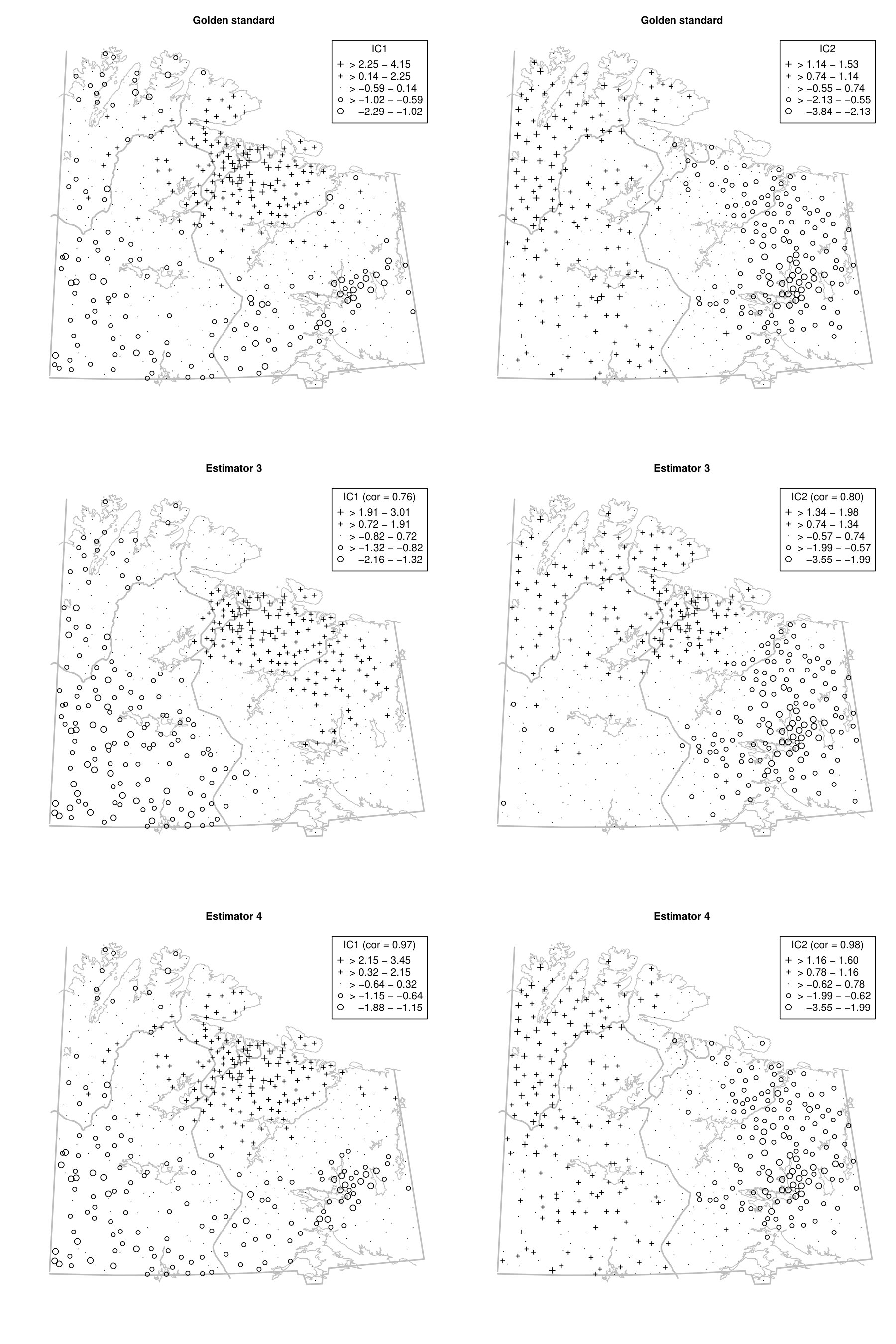 Figure 1
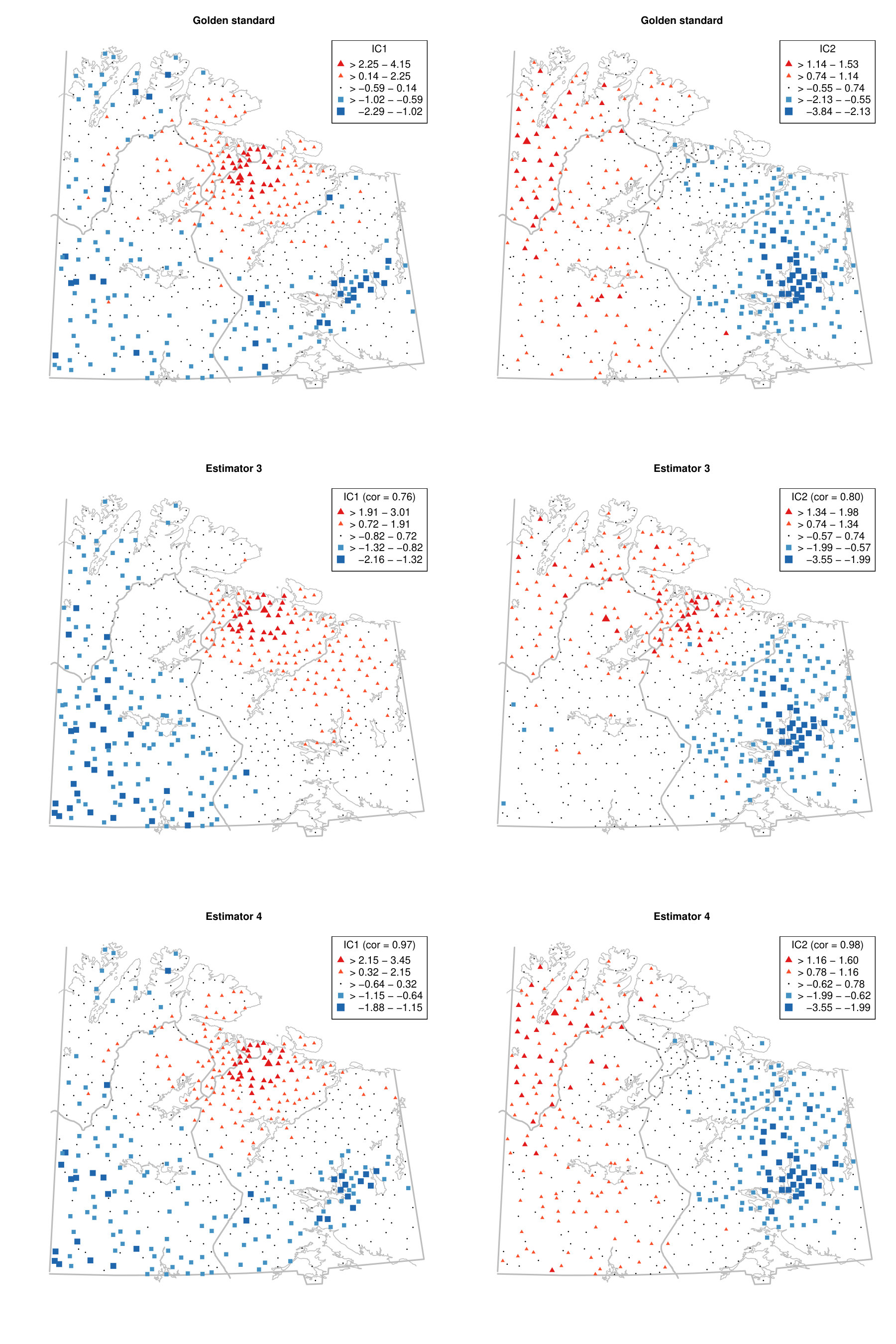 Figure 2
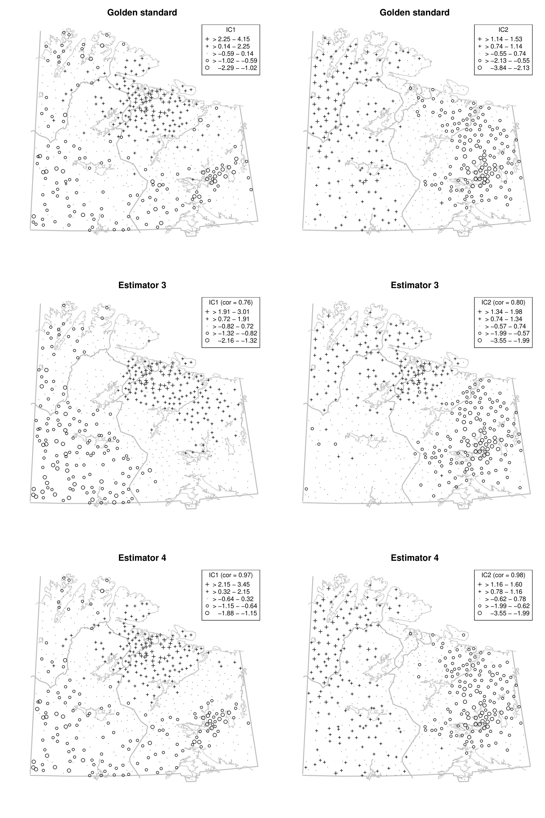 Figure 3
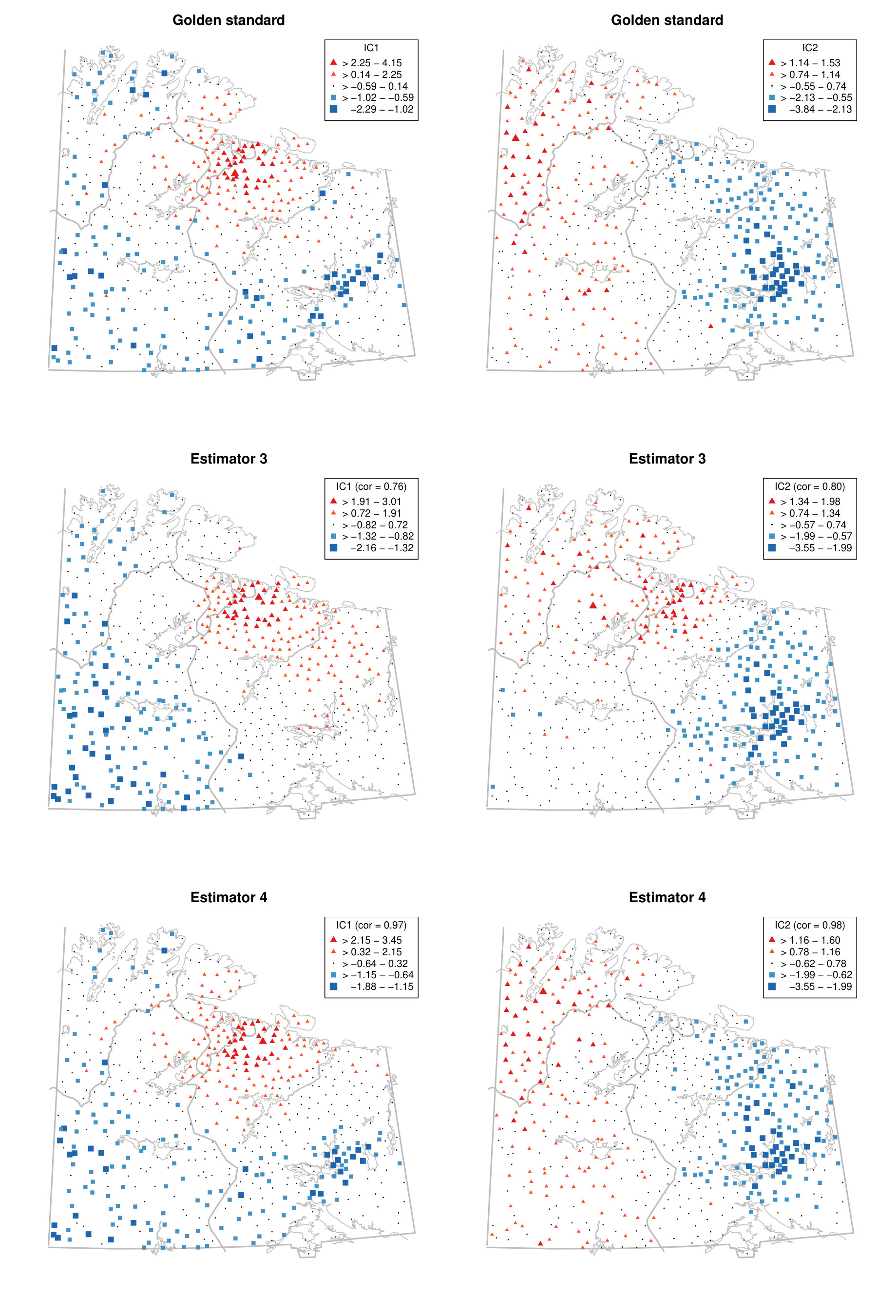 Figure 4
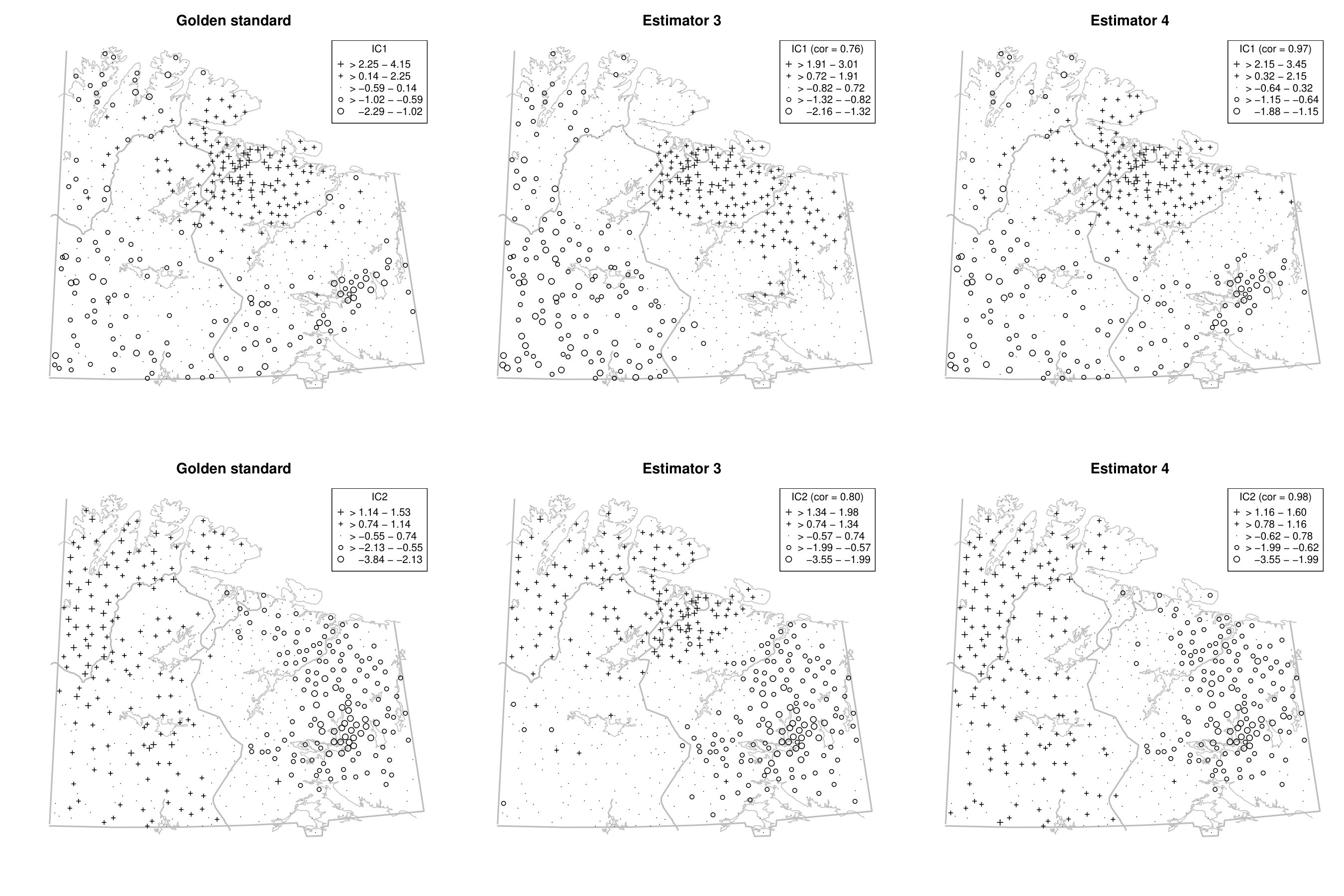 Figure 5
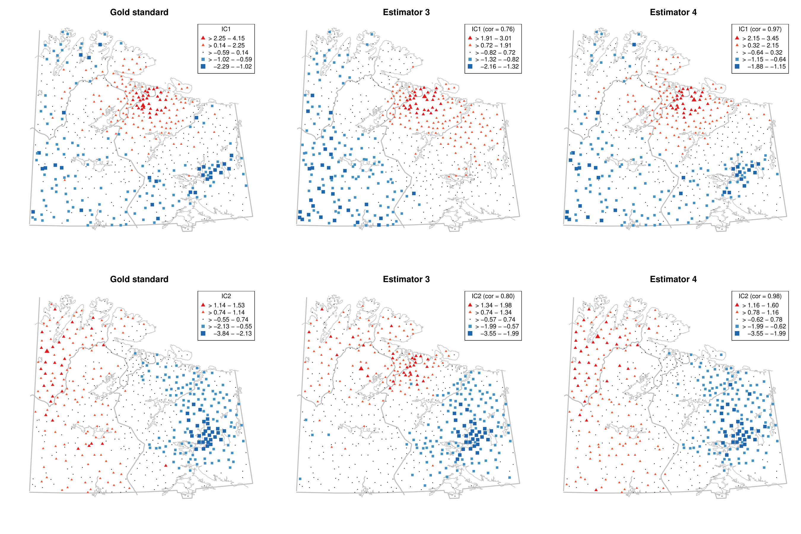 Figure 6
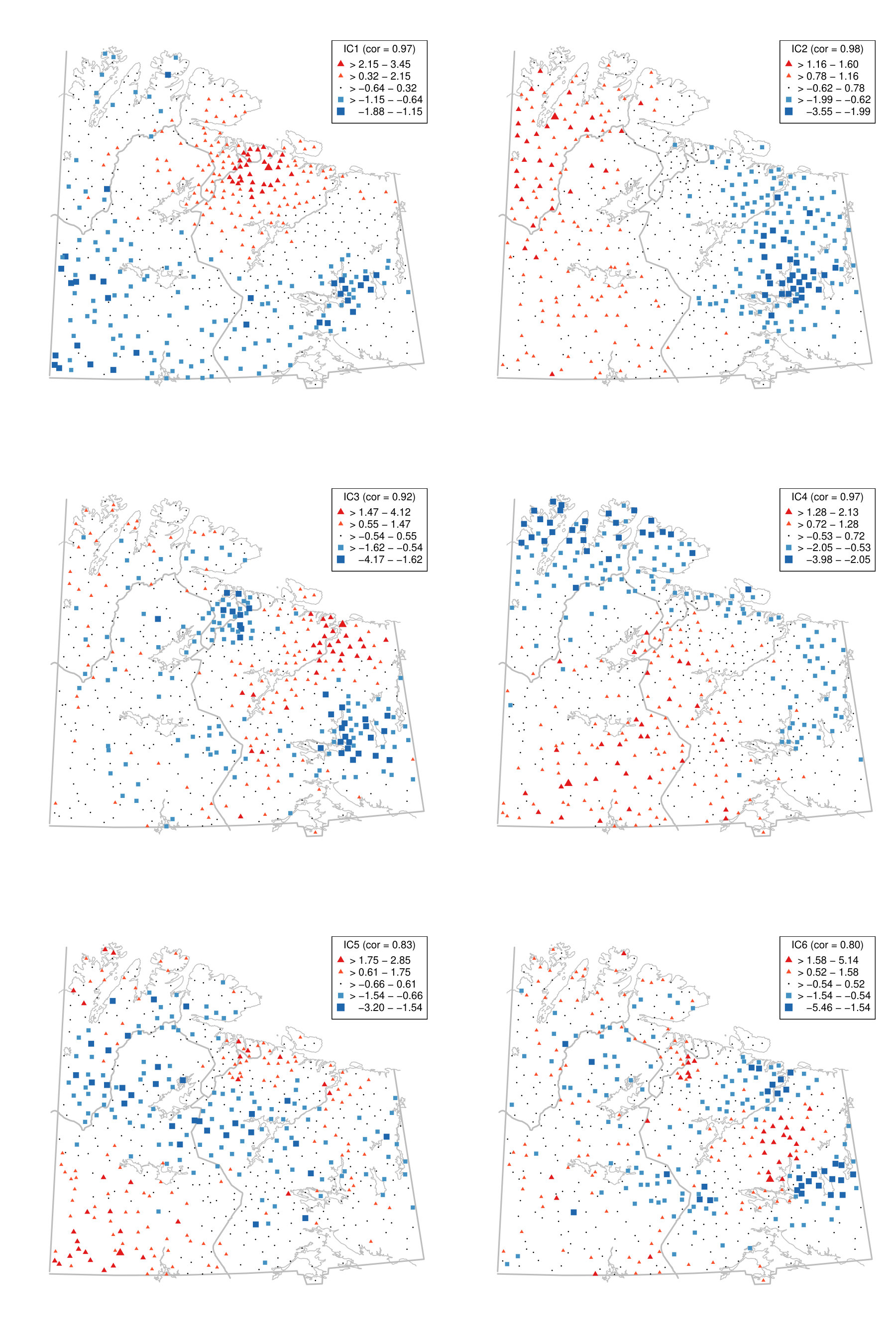 Figure 7
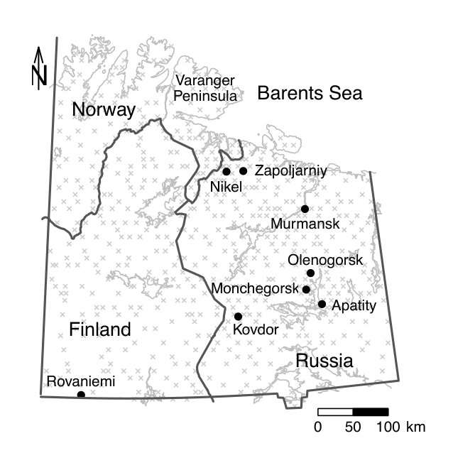 Figure 8
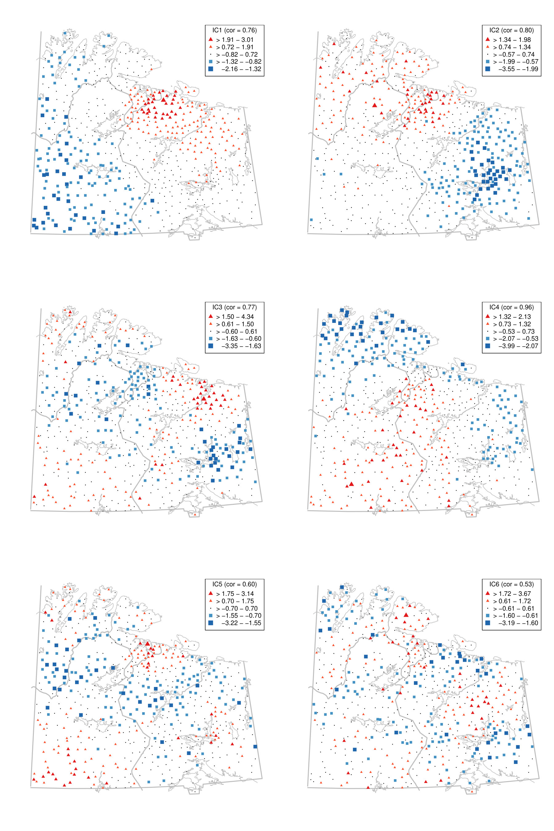 Figure 9
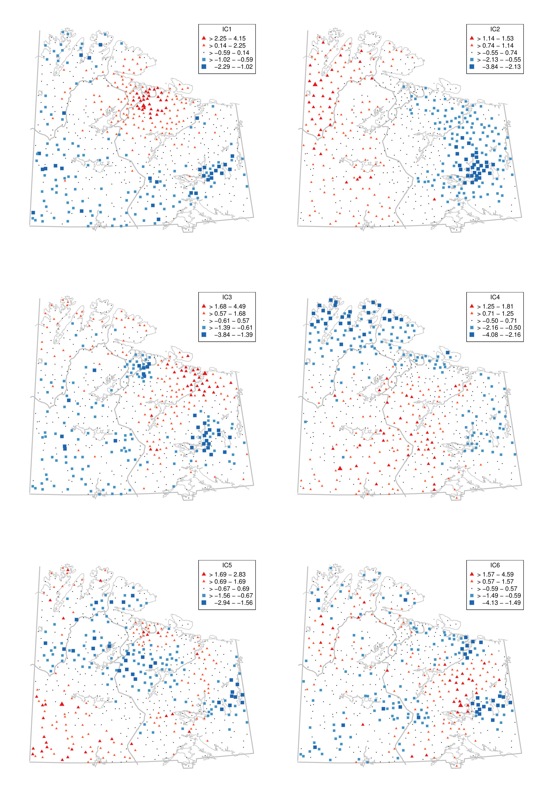 Figure 10
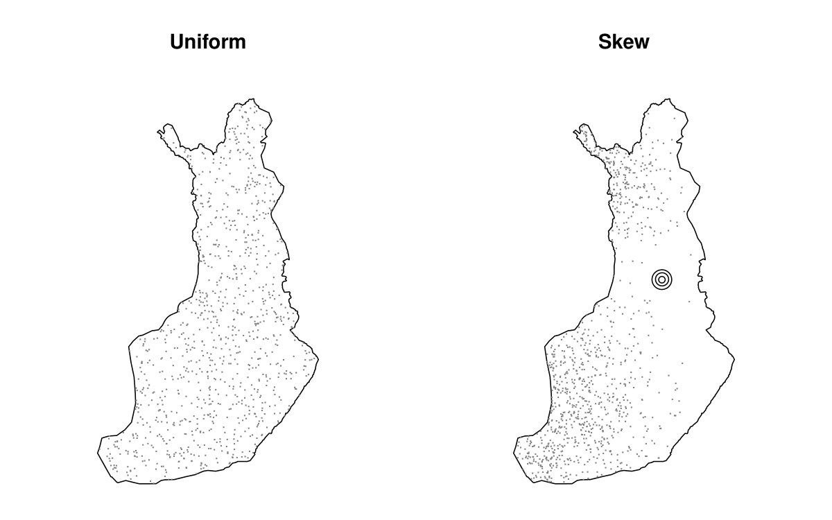 Figure 11
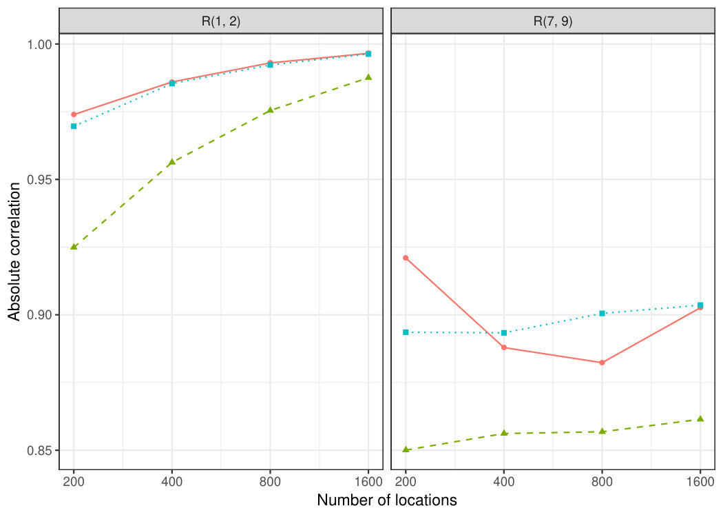 Figure 12
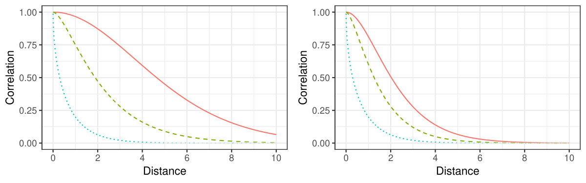 Figure 13
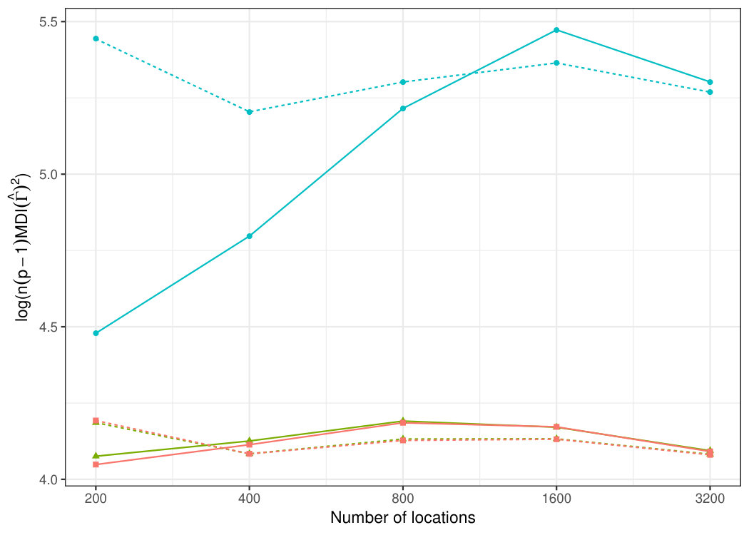 Figure 14
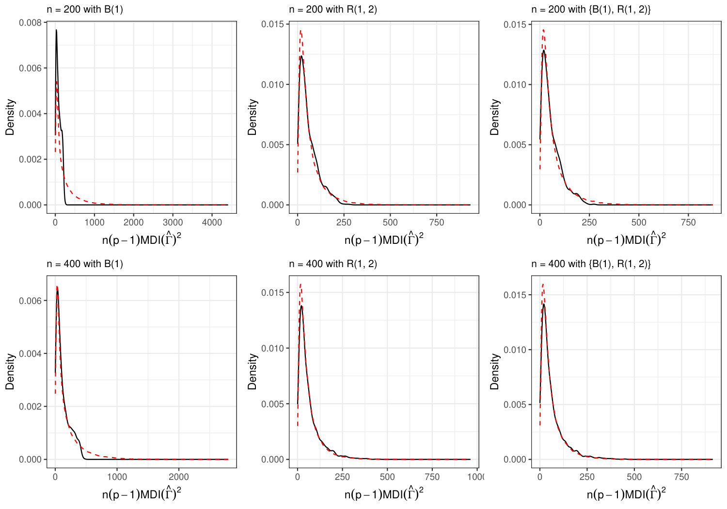 Figure 15
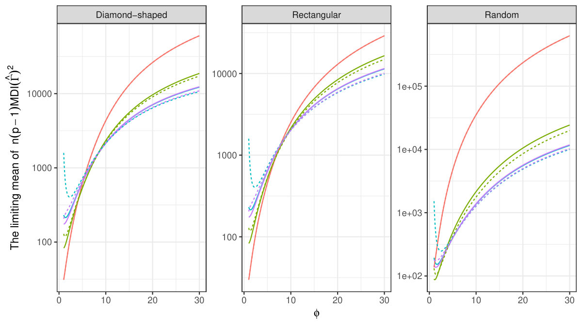 Figure 16
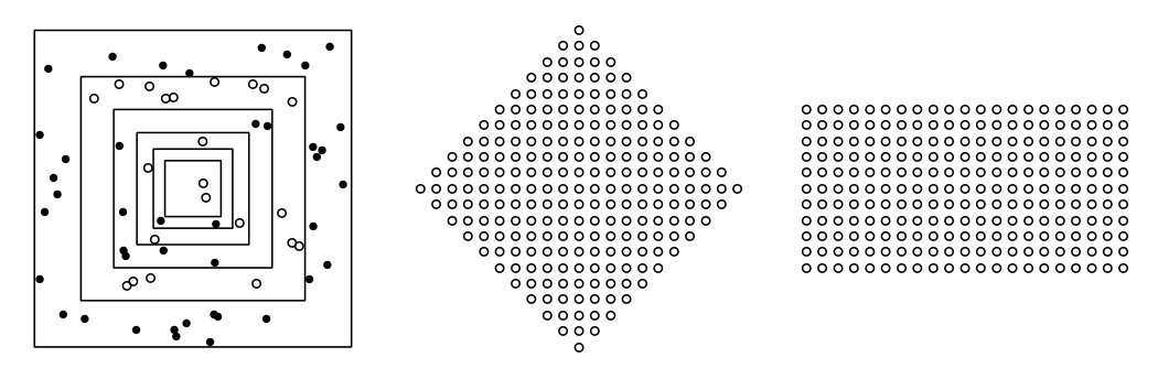 Figure 17
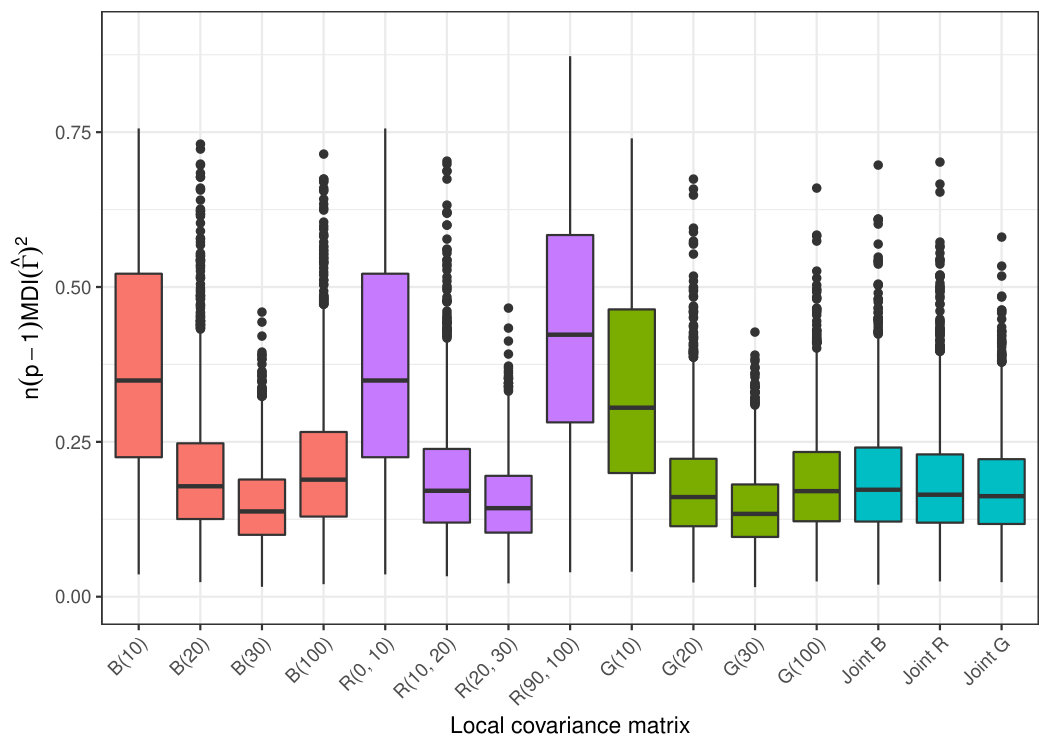 Figure 18
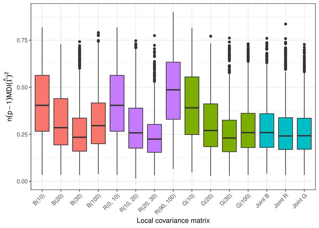 Figure 19
Peer Reviews
No public reviews on file for this paper yet. If you reviewed it on a platform where reviews are public (OpenReview, ICLR, NeurIPS, ICML), you can paste yours below so the community can read it here.
Videos
No videos yet. Explain this paper in a talk, walkthrough, or lecture? Add one.
Taxonomy
TopicsBlind Source Separation Techniques · Spectroscopy and Chemometric Analyses · Speech and Audio Processing
\AtAppendix\AtAppendix\AtAppendix\AtAppendix\AtAppendix\AtAppendix
Spatial blind source separation
François BACHOC
Institut de Mathématiques de Toulouse, Université Paul Sabatier,
118 route de Narbonne, 31062 Toulouse, France
Marc G. GENTON
Statistics Program, King Abdullah University of Science and Technology,
Thuwal 23955-6900, Saudi Arabia
Klaus NORDHAUSEN
CSTAT, Vienna University of Technology,
Wiedner Hauptstr. 7, A-1040 Vienna, Austria
Anne RUIZ-GAZEN
Toulouse School of Economics, University of Toulouse Capitole,
21 allée de Brienne, 31000 Toulouse, France
Joni VIRTA
Department of Mathematics and Statistics, University of Turku,
20014 Turun yliopisto, Finland,
Department of Mathematics and Systems Analysis, Aalto University,
PL 11000, 00076 AALTO, Finland.
Abstract
Recently a blind source separation model was suggested for spatial data together with an estimator based on the simultaneous diagonalisation of two scatter matrices. The asymptotic properties of this estimator are derived here and a new estimator, based on the joint diagonalisation of more than two scatter matrices, is proposed. The asymptotic properties and merits of the novel estimator are verified in simulation studies. A real data example illustrates the method.
keywords:
Joint diagonalisation; Limiting distribution; Multivariate random field; Spatial scatter matrix.
1 Introduction
There is an abundance of multivariate data measured at spatial locations in a domain . Such data exhibit two kinds of dependence: measurements taken closer to each other tend to be more similar than measurements taken further apart, and the variable values within a single location are likely to be correlated.
This complexity makes modelling multivariate spatial data computationally and theoretically difficult due to the large number of parameters required to represent the dependencies. In this work we address this problem through blind source separation, a framework established as independent component analysis for independent and identically distributed data and for stationary and non-stationary time series; see Comon & Jutten (2010) and Nordhausen & Oja (2018). Denoting a -variate random field as , where T is the transpose operator, we assume that obeys the spatial blind source separation model introduced in Nordhausen et al. (2015). That is, at a location is a linear mixture of an underlying -variate latent field with independent components,
[TABLE]
where is an unknown full rank matrix. In this introduction section, we consider that the random fields and have mean functions zero, for the sake of simplicity.
When the observed random field takes the form (1.1), modeling and computational simplifications can be obtained. Indeed, if no assumption at all is made on , then the distribution of is characterized by covariance functions and by cross-covariance functions. In contrast, when it is assumed that takes the form (1.1), then the distribution of is characterized by covariance functions and by a matrix. As a function is an infinite-dimensional object, it is more difficult to model and estimate than a fixed-dimensional matrix. Thus, when the observed random field takes the form (1.1), modeling simplifications are available.
When no assumption is made on , a common practice in geostatistics is to let each of the covariance functions and each of the cross-covariance functions of be characterized by parameters. For instance the case can correspond to a variance and a length scale parameter for an isotropic function. Then, the resulting parameters are usually estimated jointly by optimizing a fit criterion, typically the likelihood (Genton & Kleiber, 2015). This requires to perform an optimization in dimension , where the computational cost of an evaluation of the likelihood is . Once the parameters are estimated, the prediction of for new values of can be performed at the computational cost .
In contrast, consider that model (1.1) holds for . We will show in this paper that an estimate of can be obtained. This is carried out by, first, computing scatter matrices with computational cost and, second, performing an optimization in dimension where the computational cost of the function to be evaluated is , see § 4 for details. If each covariance function of is characterized by parameters, each of them can be estimated separately, by optimizing the likelihood in dimension . The evaluation cost of the likelihood is . Once the covariance parameters are estimated, the prediction of for new values of can be performed at cost . Indeed, the predictions of can be performed separately at cost and aggregated with negligible cost.
Not all random fields obey a spatial blind source separation model of the form (1.1). For instance, (1.1) forces the cross-covariance functions of to be symmetric. Nevertheless, it is a reasonable assumption in a fair number of practical situations (Nordhausen et al., 2015) and brings the computational benefits discussed above. Furthermore, an additional benefit of the form (1.1) is dimension reduction. In blind source separation, often significantly fewer than the full latent components are needed to capture the essential structure of the original observations and the remaining components can be discarded as noise.
We thus consider the spatial blind source separation model (1.1) in this paper and focus on the estimation of . As discussed above, this estimation enables to estimate the cross-covariance functions of and to perform prediction. Our approach for estimating is based on the use of local covariance, or scatter, matrices,
[TABLE]
where is called the kernel function. Nordhausen et al. (2015) obtained estimators of through a generalized eigendecomposition of pairs of local covariance matrices with kernels of the form , with , for a positive constant , where denotes the indicator function and . Their estimators were based on the following definition, with for some .
Definition 1.1**.**
An unmixing matrix estimator jointly diagonalizes and in the following way
[TABLE]
*where is a diagonal matrix with diagonal elements in decreasing order. *
This method is conceptually close to principal component analysis where latent variables that have maximal variance are found through the diagonalisation of the covariance matrix. However, since the covariance matrix does not capture spatial information, it was extended to the concept of a local covariance matrix in Nordhausen et al. (2015). Analogously, diagonalising local covariance matrices then aims to find latent fields that maximize spatial correlation.
Here, we expand on their work by not restricting the kernel in Definition 1.1 to be of the “ball” form . Furthermore, we derive the asymptotic behavior for the method proposed in Nordhausen et al. (2015) for a large class of kernel functions .
The idea when constructing these kernel functions is that the mean values of and would be diagonal matrices if, in their definition, the mixed components were replaced by the latent components . Hence, a general blind source separation strategy is to undo the mixing in by finding a matrix which simultaneously diagonalizes and . This is computationaly simple and can always be done exactly using generalized eigenvalue-eigenvector theory. From temporal blind source separation, it is however well known that when diagonalising only two matrices, the choice of the matrices can have a large impact on the separation efficiency. Therefore, it is a popular strategy to approximately diagonalize more than two matrices with the hope of including more information; see for example Belouchrani et al. (1997), Nordhausen (2014), Miettinen et al. (2014), Matilainen et al. (2015) and Miettinen et al. (2016). Approximate diagonalization becomes then necessary as the matrices commute only at the population level but not when estimated using finite data. There are many algorithms available for this purpose. We use this idea to extend the method of Nordhausen et al. (2015) to jointly diagonalize more than two local covariance matrices. We also derive the asymptotic behaviour of these novel estimators.
2 Spatial blind source separation model
2.1 General assumptions
In the spatial blind source separation model, the following assumptions are made: {assumption} for ;
{assumption} ;
{assumption} , where is a diagonal matrix whose diagonal elements depend only on .
Let , where denotes the stationary covariance function of , for .
Assumption 2.1 is made for convenience and can easily be replaced by assuming a constant unknown mean (see Lemma B.31 in the supplementary material). Assumption 2.1 says that the components of are uncorrelated and implies that the variances of the components are one, which reduces identifiability issues and comes without loss of generality. Assumption 2.1 says that there is also no spatial cross-dependence between the components. However, even after these assumptions are made, the model is not uniquely defined. The order of the latent fields and also their signs can be changed. This is common for all blind source separation approaches and is not considered a problem in practice.
2.2 Identifiability
The expectations of and are respectively
[TABLE]
Thus the empirical procedure of Definition 1.1, operating on and , can be associated to the following theoretical procedure, operating on and .
Definition 2.1**.**
For any function , an unmixing matrix functional is defined as a functional which jointly diagonalizes and in the following way
[TABLE]
*where is a diagonal matrix with diagonal elements in decreasing order. *
We remark that an unmixing matrix can be found using the generalized eigenvalue-eigenvector theory. In addition, an unmixing matrix is never unique, since if and satisfy Definition 2.1, then and also satisfy Definition 2.1 for any diagonal matrix with diagonal elements equal to or . We also remark that is not the expectation of , in general. Indeed, Definitions 1.1 and 2.1 are based on non-linear functions of and of .
The usual notion of identifiability in blind source separation is that any unmixing functional should recover the components of up to signs and order of the components. Thus, any unmixing functional should coincide with , up to the order and signs of the rows.
Definition 2.2**.**
*We say that the unmixing problem given by is identifiable if any unmixing functional satisfying Definition 2.1 can be written as , where is a permutation matrix and is a diagonal matrix with diagonal elements equal to or . *
The motivation behind identifiability is that, if identifiability holds, then estimating and consistently by and enables to obtain , which will be approximately equal to a matrix of the form , with and as in Definition 2.2. The following proposition provides a necessary and sufficient condition for identifiability. This proposition is proved in § B.2 of the supplementary material. All the other theoretical results in this paper are also proved in the supplementary material. Let denote the inverse of the transpose of .
Proposition 2.3**.**
*The unmixing problem given by is identifiable if and only if the diagonal elements of are distinct. *
We remark that identifiability is a joint property of the kernel and the covariance functions . For instance, consider the situation where are compactly supported and equal to zero at distances larger than , and where one uses the function , with as kernel. Then identifiability does not hold because is equal to the zero matrix. On the other hand, if is a ball kernel of the form with , then identifiability may hold, for the same covariance functions .
Finally, for any kernel , a necessary condition for identifiability is that there does not exist , , such that for all . Indeed, if this was the case, then the diagonal elements and of would be equal, for any kernel . An extreme example of this issue is with only Gaussian components. If this is the case, then, for any orthogonal matrix , the distribution of the random field is the same as that of the random field . Hence, no statistical procedure can be expected to recover the components of , even up to signs and permutations, when only observing the transformed random field .
2.3 Relationships with other models of multivariate random fields
The spatial blind source separation is notably different from the usual multivariate models for spatial data, which are often defined starting with their covariance functions contained in a cross-covariance matrix,
[TABLE]
whereas our approach for estimating does not need to model or estimate the covariance functions of the latent fields .
In a recent extensive review, Genton & Kleiber (2015) discussed different approaches to define cross-covariance matrix functionals and gave a list of properties and conventions that they should satisfy, for instance stationarity and invariance under rotation. As Genton & Kleiber (2015) pointed out, to create general classes of models with well-defined cross-covariance functionals is a major challenge. Multivariate spatial models are particularly challenging as many parameters need to be fitted. In textbooks such as Wackernagel (2003) usually the following two popular models are described.
In the intrinsic correlation model it is assumed that the stationary covariance matrix can be written as the product of the variable covariances and the spatial correlations, , for all lags , where is a non-negative definite matrix and a univariate spatial correlation function.
The more popular linear model of coregionalization is a generalization of the intrinsic correlation model, and the covariance matrix then has the form
[TABLE]
for some positive integer with all the ’s being univariate spatial correlation functions and ’s being non-negative definite matrices, often called coregionalization matrices. Hence, with this reduces to the intrinsic correlation model. The linear model of coregionalization implies a symmetric cross-covariance matrix.
Estimation in the linear model of coregionalization is discussed in several papers. Goulard & Voltz (1992) focused on the coregionalization matrices using an iterative algorithm where the spatial correlation functions are assumed to be known. The algorithm was extended in Emery (2010). Assuming Gaussian random fields, an expectation-maximisation algorithm was suggested in Zhang (2007) and a Bayesian approach was considered in Gelfand et al. (2004).
There is a simple connection between the spatial blind source separation model and the linear model of coregionalization. The covariance matrix resulting from a spatial blind source separation model is always symmetric and can be written as
[TABLE]
with , being the th column of . Thus the spatial blind source separation model is a special case of the linear model of coregionalization with and where all coregionalization matrices , , are rank one matrices.
3 Asymptotic properties for simultaneous diagonalisation of two matrices
Recall the definition (1.2) of a local covariance matrix and that
[TABLE]
is the covariance estimator. Asymptotic results can be derived for the previous estimators assuming that Assumptions 1 to 3 hold together with the following assumptions: {assumption} The coordinates of are stationary Gaussian processes on ;
{assumption} A fixed exists so that, for all and, for all , , ;
{assumption} Fixed and exist such that, for all and, for all ,
[TABLE]
{assumption}
Assuming Assumption 3.1 holds, then for the same and we have
[TABLE]
{assumption}
We have
[TABLE]
Assumption 3.1 implies that is unbounded as , which means that we address the increasing domain asymptotic framework (Cressie, 1993).
Assumption 3 holds in particular for the function and for the “ball” and “ring” kernels with fixed and with fixed .
Up to reordering the components of , which comes without loss of generality, Assumption 3 is an asymptotic version of the identifiability condition in Proposition 2.3. Under Assumption 3, identifiability in the sense of Definition 2.2 holds for sufficiently large , from Proposition 2.3.
Proposition 3.1 below gives the consistency of the estimator , where satisfies Assumption 3. The proof of this proposition is provided in § B.4 of the supplementary material.
Proposition 3.1**.**
*Suppose and Assumptions 2.1 to 3.1 hold and let satisfy Assumption 3. Then in probability when . *
We remark that depends on and that we do not assume that the sequence of matrices converges to a fixed matrix as . Hence, Proposition 3.1 shows that converges to zero, and not that converges to .
Next, we show the joint asymptotic normality of and , seen as sequences of random vectors. Similarly as in Proposition 3.1, we do not need to assume that the sequence of covariance matrices of these two sequences of vectors converges to a fixed matrix. Hence, we will not show that these sequences of random vectors converge jointly to a fixed Gaussian distribution. Instead, we will show that the distances between the distributions of these random vectors and Gaussian distributions converge to zero as . As a distance between distributions, we consider a metric generating the topology of weak convergence on the set of Borel probability measures on Euclidean spaces (see, e.g., Dudley (2002), p. 393). The benefit of such a distance is that a sequence of distributions converges to a fixed distribution if and only if converges to zero. The next proposition provides the asymptotic normality result. It is proved in § B.4 of the supplementary material.
Proposition 3.2**.**
Assume the same assumptions as in Proposition 3.1. Let be the vector of size , defined for , , by
[TABLE]
Let be the distribution of . Then, as ,
[TABLE]
*where denotes the normal distribution and details concerning the matrix are given in Appendix A.2. Furthermore, the largest eigenvalue of is bounded as . *
In Proposition 3.2, is a matrix that depends on and is interpreted as an asymptotic covariance matrix. Also, in Proposition 3.2, the vectors and , that are asymptotically Gaussian, are obtained by row vectorization of and . Taking with in Propositions 3.1 and 3.2 gives the asymptotic properties of the method proposed in Nordhausen et al. (2015).
Remark 3.3**.**
*Propositions 3.1 and 3.2 remain valid when centering the process by . Indeed, we prove in Lemma B.31 of the supplementary material that the difference between the centered estimator and is of order . *
For a matrix with rows , let be the row vectorization of and for a matrix of size , let . Next, Proposition 3.4 shows the joint asymptotic normality of the estimators and . This proposition is proved in § B.4 of the supplementary material.
Proposition 3.4**.**
Assume the same assumptions as in Proposition 3.1. Assume also that Assumption 3 holds. For and in Definition 1.1, let be the distribution of
[TABLE]
Then, we can choose and in Definition 1.1 so that when ,
[TABLE]
*where details concerning the matrix are given in Appendix A.3. *
In Proposition 3.4, similarly as before, we consider the sequences of vectors obtained by vectorizing and taking the diagonal of . Again, we do not show that the sequence of joint distributions of these vectors converges to a fixed distribution. Instead, we show that these joint distributions are asymptotically close to Gaussian distributions, with covariance matrices given by . We remark that denotes a sequence of matrices. We also remark that, in Definition 1.1, is not uniquely defined. It is defined up to the signs of its rows. Hence, Proposition 3.4 shows that there exists a choice of the sequence in Definition 1.1 such that asymptotic normality holds as .
The performance of the estimators and depends on the choice of that should be chosen so that has diagonal elements as distinct as possible. This is similar to the time series context as described in Miettinen et al. (2012). To avoid this dependency in the time series context, the joint diagonalisation of more than two matrices has been suggested and we will apply this concept to the spatial context in the following section.
4 Improving the estimation of the spatial blind source separation model by jointly diagonalising more than two matrices
Spatial blind source separation with more than two kernel functions of the form , with , can be formulated as
[TABLE]
We can show that, if , the set of satisfying (4.1) coincides with the set of satisfying Definition 1.1. From experience in time series blind source separation (see for example Miettinen et al., 2016), usually the diagonalisation of several matrices gives a better separation than those based on two matrices only. In this paper, we indeed show that using is beneficial from a theoretical point of view and in practice.
The identifiability notion of Definition 2.2 and Proposition 2.3 can be extended to the case of more than two local covariance matrices. We first remark that the theoretical version of (4.1) is
[TABLE]
We then extend Definition 2.2 and Proposition 2.3 to the case of more than two local covariance matrices.
Definition 4.1**.**
*We say that the unmixing problem given by is identifiable if any unmixing functional satisfying (4.2) can be written as , where is a permutation matrix and is a diagonal matrix with diagonal elements equal to or . *
Proposition 4.2**.**
*The unmixing problem given by is identifiable if and only if for every pair , , there exists such that . *
Proposition 4.2 is proved in § B.5 of the supplementary material. We remark that the identifiability condition in Proposition 4.2 is weaker than that in Proposition 2.3, because if the condition in Proposition 2.3 holds with being one of the , then the condition in Proposition 4.2 holds. This is one of the benefits of jointly diagonalising more than two matrices.
One of the main theoretical contributions of this paper is to provide an asymptotic analysis of the joint diagonalisation of several matrices in the spatial context. Assumption 3, on asymptotic identifiability, can be replaced by the following weaker assumption.
{assumption}
A fixed and exist so that for all , , for every pair , , there exists , such that .
In the next proposition, we prove the consistency of . This proposition is proved in § B.6 of the supplementary material.
Proposition 4.3**.**
*Suppose Assumptions 2.1 to 3.1 hold. Let be fixed. Let satisfy Assumption 3. Assume that Assumption 4 holds. Let satisfy (4.1). Then we can choose so that in probability when goes to infinity. *
In Proposition 4.3, we remark that is defined only up to permutation of the rows and multiplications of them by or . Hence, we show that there exists a choice of a sequence that converges to . The next proposition provides an asymptotic normality result. It is proved in § B.6 of the supplementary material.
Proposition 4.4**.**
Assume the same assumptions as in Proposition 4.3. Let be any sequence of matrices so that for any , satisfies (4.1). Then, a sequence of permutation matrices and a sequence of diagonal matrices exist, with diagonal components in , so that the distribution of with satisfies, as ,
[TABLE]
*where details concerning the matrix are given in Appendix A.4. *
In Proposition 4.4, for any , the choice of satisfying (4.1) is not unique. The proposition shows that, for any choice of the sequence of matrices , one can exchange the rows and multiply them by or , to obtain a sequence of matrices that converges to as . Furthermore, similarly as in Proposition 3.4, we show that the sequence of distributions of is asymptotically close to a sequence of Gaussian distributions. The sequence of covariance matrices of these Gaussian distributions is .
The idea of joint diagonalisation is not new in spatial data analysis. For example in Xie & Myers (1995), Xie et al. (1995) and De Iaco et al. (2013), in a model-free context, matrix variograms have been jointly diagonalized. However, the unmixing matrix was restricted to be orthogonal, which would therefore not solve the spatial blind source separation model.
While two symmetric matrices can always be simultaneously diagonalized, this is usually not the case for more than two matrices which are estimated based on finite data. Therefore, algorithms are needed for approximate joint diagonalisation. In this paper we use an algorithm which is based on Givens rotations (Clarkson, 1988). Other possible algorithms and their impact on the properties of the estimates are for example discussed in Illner et al. (2015).
5 Simulations
5.1 Preliminaries
In this section we use simulated data to verify our asymptotic results and to compare the efficiencies of the different local covariance estimates under a varying set of spatial models. All simulations are performed in R (R Core Team, 2019) with the help of the packages geoR (Ribeiro Jr & Diggle, 2016), JADE (Miettinen et al., 2017) and RcppArmadillo (Eddelbuettel & Sanderson, 2014). To generate the simulation data, we have chosen some particular covariance functions for the latent fields. However, our proposed methods do not use this information in any way, but operate solely through the selection of local covariance matrices.
5.2
Asymptotic approximation of the unmixing matrix estimator
We start with a simple simulation to establish the validity of the asymptotic approximation of the unmixing matrix estimator for different kernels and to obtain some preliminary comparative results between the proposed estimators. We consider a centered, three-variate spatial blind source separation model where each of the three independent latent fields has a Matérn covariance function with shape and range parameters (\kappa,\phi)\in\{(6,\text{1\cdot2}),(1,\text{1\cdot5}),(\text{0\cdot25},1)\}, which correspond to the left panel in Fig. 5.1. We recall that the Matérn correlation function is defined by
[TABLE]
where is the shape parameter, is the range parameter and is the modified Bessel function of the second kind of order . Our location pattern is constructed in the following way: the first 200 locations are drawn uniformly random from an origin-centered square of side length units. For the next 200 locations, we scale the side length of the square by the factor to obtain the larger square and draw the points uniformly random on . Next, we always scale the side length of the previous square by to obtain and draw the same amount of locations we already have on , thus doubling the number of points every time. This process is continued until we have obtained a total of locations. In the simulation we consider the sample sizes , for , each time using the first of the points, that is, all points inside the th innermost square on the left-hand side of Fig. 5.2. The six samples then correspond to nested samples of points and represent the increasing domain asymptotic scheme implied by Assumption 3.1.
We expect any successful unmixing estimator to satisfy up to sign changes and row permutations. The minimum distance index (Ilmonen et al., 2010b) is defined as,
[TABLE]
where is the set of all matrices with exactly one non-zero element in each row and column and is the Frobenius norm. The minimum distance index measures how close is to the identity matrix up to scaling, order and signs of its rows, and with lower values indicating more efficient estimation. Moreover, for any such that for some limiting covariance matrix , the transformed index converges to a limiting distribution where are independent chi-squared random variables with one degree of freedom and are the non-zero eigenvalues of the matrix,
[TABLE]
where and is the matrix with one as its th element and the rest of the elements equal zero, and is the usual tensor matrix product. In particular, the expected value of the limiting distribution is the sum of the limiting variances of the off-diagonal elements of . This provides us with a useful single-number summary to measure the asymptotic efficiency of the method, i.e., the mean value of over several replications.
Following the argument of the proof of Proposition B.17 in the supplementary material, our spatial blind source separation estimators are affine equivariant. More precisely, let be computed from according to (4.1) and recall that is computed from according to (4.1). Then we have , up to sign changes and row permutations. In this sense, is invariant to the value of . As the minimum distance index depends on only through , it is thus without loss of generality that we may consider throughout § 5 only the trivial mixing case . Taking different into consideration would give exactly the same results as those provided below.
Recall that the ball and ring kernels are defined as and for fixed and . We simulate 2000 replications for each sample size and estimate the unmixing matrix in each case with three different choices for the local covariance matrix kernels: and , where the argument is dropped and the brackets denote the joint diagonalisation of the kernels inside. The latent covariance functions on the left panel of Fig. 5.1 show that the dependencies of the last two fields die off rather quickly, and we would expect that already very local information is sufficient to separate the fields. Moreover, out of all one-unit intervals, the magnitudes of the three covariance functions differ the most from each other in the interval from 1 to 2 and we may reasonably assume that either or will be the most efficient choice.
The mean values of over the 2000 replications are shown as the solid lines in Fig. 5.3, with the dashed lines representing the asymptotic approximated values of the means, towards which they are expected to converge (see Propositions 3.4 and 4.4). As evidenced in Fig. 5.3, this is indeed what happens. For the reasons detailed in the previous paragraph, the kernel is notably a more efficient choice than . However, the ball kernel still carries some additional information to the ring as their joint diagonalisation, , gives the best results out of the three choices, albeit marginally. As the main purpose of the current simulation was to verify the limiting theorems and compare the different choices of kernels, the estimation accuracy of the sources was considered jointly, through the minimum distance index. However, as it is possible that some of the individual sources are more difficult to estimate than others, we have included in § C.2 of the supplementary material a simulation study exploring individual component recovery.
The previous investigation and Fig. 5.3 used only the expected value of the asymptotic distribution. In Fig. C.1 of the supplementary material, we have also plotted the estimated densities of for all local covariance matrices and a few selected sample sizes and compared with the density of the asymptotic approximation estimated from a sample of 100,000 random variables drawn from the corresponding distributions. Overall, the two densities fit each other rather well, especially for the local covariance matrices involving the ring kernel. This shows that the asymptotic approximation to the distribution of is good already for small sample sizes.
5.3 The effect of range on the efficiency
The second simulation explores the effect of the range of the latent fields on the asymptotically optimal choice of local covariance matrices. The comparisons between the estimators are made on the basis of the expected values of the asymptotic approximations to the distribution of (that is, using the equivalent of the dashed lines in Fig. 5.3), meaning that no randomness is involved in this simulation.
We consider three-variate random fields , where and the latent fields have Matérn covariance functions with respective shape parameters \kappa=2,1,\text{0\cdot25} and a range parameter \phi\in\,\{\text{1\cdot0},\text{1\cdot1},\text{1\cdot2},\ldots,\text{30\cdot0}\}. The three covariance functions are shown for in the right panel of Fig. 5.1. The random field is observed at three different point patterns: diamond-shaped, rectangular and random, which was simulated once and held fixed throughout the study. The diamond-shaped point pattern has a radius of and a total of locations, whereas the rectangular point pattern has a “radius” of with a total of locations. In both patterns, the horizontal and vertical distance between two neighbouring locations is one unit and examples of the two pattern types are shown in the middle and right panels of Fig. 5.2 with a radius . A rectangular pattern with “radius” is defined to have the width and the height . The random point pattern is generated simply by simulating points uniformly in the rectangle . We consider a total of eight different local covariance matrices, for , and the joint diagonalisations of the previous sets: and .
The results of the simulation are displayed in Fig. 5.4 where the two joint diagonalisations are denoted by having value “J” as the parameter . Recall that the lower the value on the -axis, the better that particular method is at estimating the three latent fields. The relative ordering of the different curves is very similar across all three plots, and it seems that the choice of the location pattern does not have a large effect on the results. In all the patterns, the local covariance matrices with either or are the best choices for small values of the range but they quickly deteriorate as increases. The opposite happens for the local covariance matrices with ; they are among the worst for small and relatively improve with increasing . The joint diagonalisation-based choices fall somewhere in-between and are never the best nor the worst choice. However, they yield performance very close to the best choice in the right end of the range-scale and are close to the optimal ones in the left end. Thus, their use could be justified in practice as the “safe choice”. Comparing the two types of local covariance matrices, balls and rings, we observe that in the majority of cases the rings prove superior to the balls.
5.4 Efficiency comparison
To compare a larger number of local covariance matrices and their combinations, we simulate three-variate random fields , where and the latent fields have Matérn covariance functions with the shape parameters \kappa=6,1,\text{0\cdot25} and the range parameter , in kilometers. We consider two different fixed-location patterns fitted inside the map of Finland; see Fig. 5.5. The first location pattern has the locations drawn uniformly from the map and the second location pattern is drawn from a west-skew distribution. Both patterns have a total of locations and to better distinguish the scale we have added three concentric circles with respective radii of 10, 20, and 30 kilometers in the empty area of the skew map.
We simulate a total of 2000 replications of the above scheme with the fixed maps. In each case we compute the minimum distance index values of the estimates obtained with the local covariance matrix kernels , where , and the joint diagonalisation of each of the three quadruplets , and adding up to a total of 15 estimators. The Gaussian kernel is parametrized as G(r)\equiv\exp[-\text{0\cdot5}\{\Phi^{-1}(\text{0\cdot95})s/r\}^{2}], where is the distance and is the quantile function of the standard normal distribution, making have % of its total mass in the radius ball around its center. Thus, can be considered a smooth approximation of . The larger radius kernels , , are included in the simulation to investigate what happens when we overestimate the dependency radius. The mean minimum distance index values for the 15 estimators are plotted in Fig. 5.6 and show that for both maps and all local covariance types, increasing the radius yields more accurate separation results all the way up to , whereas for the results again worsen. This observation shows that when using a single local covariance matrix, the choice of the type and the radius are especially important, most likely requiring some expert knowledge on the study. However, this problem is completely averted when we use the joint diagonalisation of several matrices. For both maps and all local covariance types the joint diagonalisation produces results very comparable to the best individual matrices, even though the joint diagonalisations also include the “bad choices”, . We also observe a similar behaviour in the first and second simulation studies where, in the absence of knowledge on the optimal choice, the joint diagonalisation either is the most efficient choice or provides a performance very close to the most efficient choice. Thus, we recommend the use of the joint diagonalisation of scatter matrices with a sufficiently large variation of radii for the kernels.
Finally, a comparison between the two maps reveals that the relative behaviour of the estimators is roughly the same in both maps, but the estimation is generally more difficult in the skew map, revealed by the on average higher minimum distance index values. This is explained by the large number of isolated points which contribute no information to the estimation of the local covariance matrices, making the sample size essentially smaller than .
6 Data application
To illustrate the benefit of jointly diagonalising more than two scatter matrices from a practical point of view, we reconsider the moss data from the Kola project which are available in the R package StatDa (Filzmoser, 2015) and described in Reimann et al. (2008), for example. The data consist of 594 samples of terrestrial moss collected at different sites in north Europe on the borders of Norway, Finland and Russia. The corresponding map with sampling locations is given in the online supplement in Fig. D.1. The amount of 31 chemical elements found in the moss samples was already used as a spatial blind source separation example in Nordhausen et al. (2015) where the covariance matrix and were simultaneously diagonalized. The goal of that analysis was to reveal interpretable components exhibiting clear spatial patterns. In Nordhausen et al. (2015), the radius of 50 kilometers was carefully chosen by an expert in that analysis and considered best compared to several other radii not mentioned there. The analysis found six meaningful components, which could be used to distinguish underlying natural geological patterns from environmental pollution patterns. These six components had the six largest eigenvalues and are visualized in Fig. D.2 in the online supplement.
We show that the gold standard components can be stably estimated without subject knowledge on the optimal radius by simply jointly diagonalizing a large enough collection of local covariance matrices. To address the compositional nature of the data, we follow the same data preparation steps as in Nordhausen et al. (2015) and then compute five competing spatial blind source separation estimates. The scatters we used in addition to the covariance matrix are detailed in Table 6. Using these methods, we identify the six components with the highest correlations, in absolute values, to the six main components identified in Nordhausen et al. (2015). Table 6 gives the correlations of the six components.
The table shows that when using only two scatters, estimators 1, 2 and 3, some components cannot be easily found. However, when jointly diagonalising more than two scatters, the results are more stable and less dependent on the chosen distances of the scatters as can be seen for estimators 4 and 5.
This is illustrated using the gold standard and estimators 3 and 4 in Fig. A.1 in the Appendix for the first two components. For completeness, § D of the online supplement contains all six components for the three estimators. The first two components represent, according to Nordhausen et al. (2015), areas with different types of industrial contamination and Figure A.1 shows that the gold standard and estimator 4 agree quite well on these, but estimator 3 yields a different map. More precisely, the first component obtained by the gold standard and the estimator 4 highlights a cluster of negative scores around the Monchegorsk and Apatity region, which reveals the mining and processing of alkaline deposits. This cluster is not revealed by estimator 3. Similarly, the second components are similar between the gold standard and the estimator 4, but the component from the estimator 3 differs from these two, especially for the sampling locations in Finland. Thus, using several scatters gives a more stable impression whereas the maps can vary considerably when only two scatters are used, in which case subject expertise becomes more relevant.
7 Discussion
Our proposed methodology can be extended in multiple directions in future work. The assumptions of Gaussian or stationary fields could be relaxed. The spatial and temporal blind source separation methodologies could be combined to obtain spatio-temporal blind source separation. If used for dimension reduction, estimators for the number of latent non-noise fields could be devised using strategies similar to those in Virta & Nordhausen (2019). Additionally, the combination of spatial blind source separation with univariate kriging and univariate modelling warrants investigation.
How to choose the local covariance matrices optimally is also of interest. This is still an open problem for temporal blind source separation methods, such as second-order blind identification (Belouchrani et al., 1997). Several strategies have been suggested, see for example Tang et al. (2005), and many of them could be useful also in selecting the kernels in spatial blind source separation. The estimation accuracy of our proposed method is based on how well separated the eigenvalues of the matrices , , are. Since the connection between the eigenvalues and the unknown covariance functions is complicated, our suggestion, backed up also by the simulations, is to stay on the safe side and jointly use a large number of ring kernels. However, including large numbers of unnecessary kernels can still have the drawback of inducing some noise to the estimates. One way to remove the unneeded kernels would be to first obtain preliminary estimates for the latent fields using a large number of kernels jointly. Then, our asymptotic results could be used to select from a large collection of sets of kernels, the one which achieves the smallest value of ; see § 5.2. The final estimates could then be computed with this asymptotically optimal choice of kernels. A similar technique was used in the context of temporal blind source separation in Taskinen et al. (2016).
Acknowledgement
The work of Nordhausen, Ruiz-Gazen and Virta was partly supported by the CRoNoS Cost action. The work of Nordhausen was also partly supported by the Austrian Science Fund. Ruiz-Gazen acknowledges funding from the French National Research Agency (ANR) under the Investments for the Future (Investissements d’Avenir) program. The authors are very grateful for the comments by the referees which helped considerably to improve the manuscript.
\appendixone
Appendix A Appendix
A.1 Notation
Let and be the vectors defined by and , for , . Let and . Let be the th base column vector of for . For and for , let be the matrix, that we see as a block matrix composed of blocks of sizes , and with block equal to .
For , we let . We remark that for a matrix . Let . We remark that for a matrix . For , let and be the unique so that . For , let and note that for a matrix . For a matrix of size , recall that and that denotes its trace.
A.2 Expression of the matrix from Proposition 3.2
Let . Using the notation of Appendix A.1, let and be the matrices defined by, for and , with ,
[TABLE]
Let
[TABLE]
Then is equal to for .
A.3 Expression of the matrix from Proposition 3.4
From Assumption 3, there exists such that for the diagonal elements of are strictly decreasing. Write these diagonal elements as . Using the notation of Appendix A.1, for , let , , and be respectively the , , and matrices defined by
[TABLE]
[TABLE]
[TABLE]
Let
[TABLE]
Let and be respectively the and matrices defined by
[TABLE]
Let be defined as but with replaced by . Then, for , is defined as
[TABLE]
A.4 Expression of the matrix from Proposition 4.4
Let . For a diagonal matrix , let . Let and be matrices defined by, for with the notation of Assumption 4,
[TABLE]
[TABLE]
and
[TABLE]
Let be the matrix defined by , for . Let be as in Appendix A.3. Let be the matrix composed of blocks of size with block defined similarly as in Appendix A.2, but with replaced by . Then, for , is defined as
[TABLE]
A.5 Map for data application
Appendix B Proofs
B.1 Introduction
We first prove Proposition 2.3 in Section B.2. Then Section B.3 provides general results for the proofs of Propositions 3.1, 3.2, 3.4, 4.3 and 4.4. Section B.4 provides the proofs of Propositions 3.1, 3.2 and 3.4. Section B.5 provides the proof of Proposition 4.2. Section B.6 provides the proofs of Propositions 4.3 and 4.4.
Propositions 3.1, 3.2, 3.4, 4.3 and 4.4 correspond to Proposition B.7, B.9, B.17, B.27 and B.29, respectively.
B.2 Proof of Proposition 2.3
We let for . We restate Proposition 2.3 and prove it.
Proposition B.1**.**
*The unmixing problem given by is identifiable if and only if the diagonal elements of are distinct. *
Proof B.2** (of Proposition B.1 (Proposition 2.3)).**
We have that is an unmixing functional if and only if
[TABLE]
*Hence the matrix is orthogonal, and its rows provide the eigenvectors of the diagonal matrix . If the diagonal elements of are distinct, then the set of one-dimensional eigenspaces of is unique and thus where is a permutation matrix and is a diagonal matrix with diagonal elements equal to or . If there are two diagonal elements of that are equal, say the first and the second without loss of generality, then consider the block diagonal matrix with first block equal to and second block equal to . Then there is an unmixing functional such that . In this case, , which is not of the form . *
B.3 General results
Recall that and are fixed. are independent stationary Gaussian processes on with zero mean functions, unit variances and covariance functions . We have and with a fixed invertible matrix.
Let be the observation points in and let be a kernel function from into . We recall
[TABLE]
and
[TABLE]
where is the diagonal matrix defined by
[TABLE]
Let be the sup norm for . Since this norm is equivalent to the Euclidean norm, and since we work under Assumptions 3.1 to 3, we can assume without loss of generality that the following conditions hold.
{condition}
With defined in Assumption 3.1, for all and for all , , we have .
{condition}
With and defined in Assumptions 3.1 and 3, for all and for all , we have
[TABLE]
{condition}
With and defined in Assumptions 3.1 and 3, for all , we have
[TABLE]
For a matrix , denote by the element from the th row and the th column of . For a vector or a matrix , denote by the th element of and by the element from the th row and the th column of . The singular values of a matrix are denoted by and, in the case when is symmetric, the eigenvalues are denoted by . The spectral norm is given by and denotes the Frobenius norm. For a sequence of random variables , we write when converges to [math] in probability as and we write when is bounded in probability as . Let be the th base column vector of . Let be the vector defined by , for , .
Lemma B.3**.**
Under Conditions B.3 and B.3, there exists a finite constant so that for all ,
[TABLE]
Proof B.4**.**
Let denote the th row of . We have
[TABLE]
*from Condition B.3. Note also that where is the vector defined by for , . Hence, the lemma is a direct consequence of Lemma 6 in Furrer et al. (2016). *
The next theorem provides a general multivariate central limit theorem for quadratic forms of Gaussian vectors. It extends standard central limit theorems in spatial statistics, see, e.g., Bachoc (2014) or Istas & Lang (1997), by allowing cases where the sequence of covariance matrices is non-converging or asymptotically singular. The full proof is given for self-consistency, although some of the arguments have appeared previously.
Theorem B.5**.**
Let be a sequence of -dimensional centered Gaussian vectors. Let be the covariance matrix of . Assume that for all , where is a fixed finite constant. Let be fixed and let be sequences of deterministic symmetric matrices. Assume that for , for , . Let be the matrix defined for , by
[TABLE]
Let be the -dimensional vector defined for , by
[TABLE]
Let be the vector defined for , by
[TABLE]
Let be the probability measure of on . Let be the Gaussian distribution on with mean vector [math] and covariance matrix . Let denote a metric generating the topology of weak convergence on the set of Borel probability measures on ; for specific examples see the discussion in Dudley (2002) p. 393. Then we have, for ,
[TABLE]
Proof B.6**.**
Assume that when . Then there exists fixed and a subsequence so that . Let be fixed. Let . We have
[TABLE]
Hence, we see that is a non-negative matrix, and, from the assumptions on and , that . Also, . Hence, by compacity, and up to extracting a further subsequence, we can assume that and when . One can show simply that when . Hence, when ,
[TABLE]
Let us prove (B.2) . We have
[TABLE]
where we have applied the triangle inequality for the metric in the last inequality above. Hence . Thus (B.2) is proved.
We remark that the matrix is symmetric, because are assumed to be symmetric in the theorem. Hence, can be diagonalized and there exist a matrix such that and a diagonal matrix such that . Let also . Observe that follows the distribution. We have
[TABLE]
where follows the distribution. Hence letting
[TABLE]
we have
[TABLE]
If , then when . Hence, and so . Hence in distribution when .
Now, if , one can show from the Lindeberg-Feller central limit theorem that when , in distribution, see also Lemma 2 in Istas & Lang (1997).
Hence, since both of the above-considered convergences in distribution hold for any , we have, by Cramér-Wold theorem, that when , in distribution. This is in contradiction with (B.2). Hence when
[TABLE]
B.4 Asymptotics when diagonalising two matrices
The next proposition gives the consistency of .
Proposition B.7**.**
*Let Conditions B.3 and B.3 hold and let satisfy Condition B.3. Then as , in probability. *
Proof B.8**.**
Clearly . Let be fixed. In order to prove the proposition, it is sufficient to show that when , .
We have,
[TABLE]
Let be the matrix, that we see as a block matrix composed of blocks of sizes , and with block equal to . We remark that is symmetric. With this notation,
[TABLE]
The largest singular value of is bounded as . Indeed, from Gershgorin’s circle theorem, is no larger than . This maximum is no larger than . This last quantity is bounded as from Condition B.3 and from Lemma 4 in Furrer et al. (2016).
Hence is bounded by a constant . Thus, using Theorem 3.2d.3 in Mathai & Provost (1992) and the fact that is symmetric,
[TABLE]
*with from Lemma B.3. *
The next proposition is a corollary of Theorem B.5 and gives the asymptotic normality of .
Proposition B.9**.**
Let, for and , be defined as in the proof of Proposition B.7. Let and let be the matrix defined by, for and , with ,
[TABLE]
Define, for , as the matrix defined for and , with by
[TABLE]
Let
[TABLE]
Then, is symmetric non-negative definite.
Assume that Conditions B.3 and B.3 hold. Let satisfy Condition B.3. Let for , be the vector of size , defined for , , by .
Let be the distribution of . Then as
[TABLE]
*Furthermore is bounded as . *
Proposition 3.2 is a direct corollary of Proposition B.9 with and . Moreover, Proposition B.9 gives details concerning the matrix .
Proof B.10**.**
Let and . We have seen in the proof of Proposition B.7 that
[TABLE]
Hence
[TABLE]
Let us first prove that is symmetric non-negative definite. Let be defined as , but with replaced by . Let be defined similarly with replaced by . For , we have
[TABLE]
Now for , let such that and . We have, using Theorem 3.2d.3 in Mathai & Provost (1992) and the fact that and are symmetric,
[TABLE]
We show similarly that
[TABLE]
and that
[TABLE]
Hence
[TABLE]
Hence, since a square matrix is uniquely defined by its corresponding quadratic forms, it follows that is the covariance matrix of the vector
[TABLE]
Hence, is symmetric non-negative definite.
*Let us now prove (B.3). We have, from Lemma B.3 and the proof of Proposition B.7, that and are bounded as for . Hence, (B.3) is a consequence of Theorem B.5. Finally, is bounded as because each component of is bounded as . *
Our objective is now to prove Proposition 3.4, which is a central limit theorem for and .
There is an equivariance property in Definition 1.1 that we will exploit. More precisely, let and let
[TABLE]
For , let
[TABLE]
and
[TABLE]
Let and satisfy the following modification of Definition 1.1:
[TABLE]
where is a diagonal matrix with diagonal elements in decreasing order. Then, we can show that
[TABLE]
satisfy Definition 1.1. The above display is the equivariance property that we will exploit. That is, we will first show a central limit theorem for and in Lemma B.15. Then, we will use the equivariance property (B.5) to obtain, directly, a central limit theorem for and in Proposition B.17.
In the next lemma, we first show a central limit theorem for and . Recall that where are the rows of a matrix . Recall also the notation .
Lemma B.11**.**
Let Conditions B.3 and B.3 hold. Let satisfy Condition B.3. Let
[TABLE]
Let be as in Proposition B.9 but where is replaced by where is the vector defined for , , by . Let be the distribution of . Then we have
[TABLE]
*Furthermore, is bounded as . *
Proof B.12**.**
*The proof is identical to the proof of Proposition B.9. We remark that, with the notation of the proof of Proposition B.9, , for . *
Now, we show, in Lemma B.13, that the transformation given by (B.4), that defines and from and , is asymptotically linear, so to speak. This will allow us to transfer the central limit theorem for and into a central limit theorem for and , for an appropriate choice of . This argument is similar to the delta method in asymptotic statistics.
We will need the following notation. We let . We remark that for a matrix . Let . We remark that for a matrix . For , let and be the unique so that . For , let and note that for a matrix . For a matrix of size , recall that .
Lemma B.13**.**
Let Conditions B.3 and B.3 hold. Let satisfy Condition B.3. Assume that Assumption 3 holds. Remark then that there exists such that for the diagonal elements of are strictly decreasing. Write these diagonal elements as . For , let be the matrix defined by
[TABLE]
Let be the matrix defined by
[TABLE]
Let be the matrix defined by
[TABLE]
Let be the matrix defined by
[TABLE]
Then, with probability going to one as , there exist and satisfying (B.4). Furthermore, can be chosen so that as ,
[TABLE]
Proof B.14**.**
Let us assume that throughout the proof. From Proposition B.7, with probability going to one, the eigenvalues of are distinct. In the rest of the proof, we set ourselves on the event when this is the case. Then, choose and satisfying (B.4) and such that
[TABLE]
We remark that and indeed exist, since when and satisfy (B.4), one can multiply each row of by or and still satisfy (B.4).
Let
[TABLE]
and
[TABLE]
Assume that in probability when . Then there exist and a subsequence so that along
[TABLE]
One can show, as for the proof of Proposition B.7, that when . Hence, up to extracting a further subsequence, we can assume that when , , where has distinct, decreasing, eigenvalues.
From Lemma 4.3 in Sun & Sun (2002), since is diagonal, there exists a sequence of random orthogonal matrices such that is diagonal and goes to in probability and so that in probability when . Hence, the pair satisfies (B.4) with probability going to one. Furthermore, all the matrices for which and satisfy (B.4) satisfy where is a diagonal matrix with diagonal elements equal to or . Hence with probability going to one, we must have for (B.6) to be also satisfied. Hence, with probability going to one, . Hence we have finally obtained and in probability when .
The rest of the proof is similar to those given in Ilmonen et al. (2010a) and Miettinen et al. (2012). By definition of and , we have
[TABLE]
Hence
[TABLE]
Also, from Lemma B.11, we have and . Thus, we get
[TABLE]
This then yields
[TABLE]
*This is in contradiction with (B.7), by definition of , , and . Hence the proof is finished. *
From Lemmas B.11 and B.13, we now obtain a central limit theorem for and . Note that .
Lemma B.15**.**
Assume the same conditions as in Lemma B.13 and let be defined as in Lemma B.13. Let, for ,
[TABLE]
from Lemma B.13. For and satisfying (B.4), let
[TABLE]
Let be the distribution of . Let be defined as in Lemma B.11. Then, we can choose and satisfying (B.4) such that when ,
[TABLE]
Proof B.16**.**
*The lemma is a direct consequence of Lemmas B.11 and B.13. The proof is carried out by contradiction, by taking subsequences along which the bounded sequences of matrices and converge, and by applying Slutsky’s lemma. *
We now use the equivariance property (B.5) to conclude.
Proposition B.17**.**
Assume the same conditions as in Lemma B.13. Let and be defined as in Lemmas B.11 and B.15. Let be the matrix defined by
[TABLE]
Let be the matrix of size defined by
[TABLE]
For and satisfying Definition 1.1, let
[TABLE]
Let be the distribution of . Let, for with as in Lemma B.13,
[TABLE]
Then, we can choose , satisfying Definition 1.1, so that when ,
[TABLE]
Proof B.18**.**
The proof directly follows from Lemma B.15 and from (B.5). Indeed, for and satisfying the central limit theorem in Lemma B.15, we can choose and satisfying Definition 1.1 and such that
[TABLE]
*We also remark that . *
B.5 Proof of Proposition 4.2
We let for . We restate Proposition 4.2 and prove it.
Proposition B.19**.**
*The unmixing problem given by is identifiable if and only if for every pair , , there exists such that . *
Proof B.20** (of Proposition B.19 (Proposition 4.2)).**
We have that satisfies (4.2) if and only if
[TABLE]
If the condition of the proposition holds, then only orthogonal matrices of the form satisfy (B.8), with the double sum being equal to
[TABLE]
*where is a permutation matrix and is a diagonal matrix with diagonal elements equal to or , see the end of the proof of Lemma B.21 below. Assume now that there exist , , such that for , . Without loss of generality, assume that and . Then consider the block diagonal matrix with first block equal to and second block equal to . Then one can show that satisfies (B.8). In this case, satisfies (4.2), and is not of the form . *
B.6 Asymptotics when diagonalising more than two matrices
Lemma B.21**.**
Let Conditions B.3 and B.3 hold. Let be fixed. Let satisfy Condition B.3. Assume that Assumption 4 holds. Let be such that
[TABLE]
*Then we can choose so that in probability when . *
Proof B.22**.**
Let, for a orthogonal matrix with rows ,
[TABLE]
Let
[TABLE]
We observe that any orthogonal matrix can be obtained from a matrix in , by row permutation and row multiplication by or . Hence, for any , there exists so that and satisfies (B.9).
We now aim at showing that in probability as , which will conclude the proof since in probability. Assume that this is not the case. Then, there exists and a subsequence so that for all and along
[TABLE]
The matrices are bounded (this can be shown as in Proposition B.7). Hence, by compacity, up to extracting a further subsequence, we have that (B.10) holds along and, as and along , .
We let
[TABLE]
We have, from Proposition B.7 and as observed in Miettinen et al. (2016), that, as and along ,
[TABLE]
in probability as . Hence, using a standard M-estimator argument and because is compact, if the unique maximum of on is , we obtain that, as and along , in probability. This is contradictory to (B.10).
Hence, to conclude the proof, it suffices to show that the unique maximum of on is . We have
[TABLE]
Also,
[TABLE]
We next show that the identity matrix is the unique maximizer of in . To see this, consider an arbitrary orthogonal matrix which maximizes . From (B.11) we see that is a diagonal matrix for all . Then, by its non-singularity, the matrix must have a column with a non-zero first element. Call the first (from the left) such column of by . We show that all other elements of must be zero. By the previous, is an eigenvector of all and we have,
[TABLE]
for some eigenvalues , . Assume then that has a second non-zero element at some arbitrary position , meaning that both . Then we write
[TABLE]
*which in turn implies that for all . By a continuity argument, this is a contradiction with Assumption 4. As the choice of was arbitrary, the only non-zero element in is the first. Repeating now the same reasoning for other elements besides the first, we observe that each column of the maximizer must have a single non-zero element, and by its orthogonality we have for some permutation matrix and some diagonal matrix with diagonal components in . The only matrix of that form belonging to is and thus, for all with , we have . *
Lemma B.23**.**
Assume the same setting and conditions as in Lemma B.21. For a diagonal matrix , let . Let and be matrices defined by, for with the notation of Assumption 4,
[TABLE]
for ,
[TABLE]
and
[TABLE]
Then, as , there exists satisfying (B.9) so that
[TABLE]
Proof B.24**.**
Assume that throughout the proof. Let satisfy (B.9) and in probability when (the existence follows from Lemma B.21). The proof of the lemma follows the proofs of ii) in Theorem 2 of Miettinen et al. (2016) and Theorem 3 in Virta et al. (2018) and as such, we present below only some key steps.
From Lemma B.11, we have and , for all . By a continuity argument and our assumptions, we further have such that the limit matrices satisfy: there exists a fixed so that for every pair , , there exists such that . The previous convergence holds up to extracting a subsequence. We omit this step in this proof for concision, but see the proof of Lemma B.13. Finally, the rotation so that also satisfies in probability.
Then, as in Virta et al. (2018), the maximisation problem,
[TABLE]
yields the estimation equations , where
[TABLE]
where we have used the shorthand and is equal to the square matrix but with its off-diagonal elements set to zero. Linearizing the estimating equations asymptotically and vectorizing, we arrive at the following form,
[TABLE]
where is the commutation matrix satisfying , and is the column vectorization where are the columns of a matrix . The orthogonality constraint can be similarly linearized to yield,
[TABLE]
Summing (B.12) and (B.13), we obtain,
[TABLE]
where in probability, where we use the notation , . Using the fact that for any conformable matrices , we get the alternative form,
[TABLE]
Continuing as in Virta et al. (2018), each diagonal element of has a corresponding diagonal block equal to 2 in . Similarly, each pair of th and th off-diagonal elements in has a corresponding sub-matrix in of the form,
[TABLE]
where is the th diagonal element of . The inverse of the sub-matrix is
[TABLE]
showing that is invertible as by our assumptions for all distinct pairs . Thus, by Slutsky’s theorem, we obtain from (B.14) that,
[TABLE]
showing that, . Consequently, also .
Finally, we next proceed as in the proof of ii) in Theorem 2 of Miettinen et al. (2016) to obtain that, as ,
[TABLE]
and for ,
[TABLE]
*Hence, the lemma follows from the definition of . *
Lemma B.25**.**
Assume the same settings and conditions as in Lemma B.21. Let be as in Proposition B.9 with replaced by where is the vector defined by, for , , . Let . Let be the matrix, composed of blocks of sizes with block equal to for .
Let be the matrix defined by , for , with the notation of Lemma B.23. Let be as in Proposition B.17 and let, for ,
[TABLE]
Then, satisfying (B.9), with replaced by , can be chosen so that, with the distribution of , we have as
[TABLE]
Proof B.26**.**
*The proof is the same as that of Proposition B.17. In particular, for satisfying (B.9), the matrix satisfies (B.9), with replaced by . *
Proposition B.27**.**
*Assume the same settings and conditions as in Lemma B.21. Let be any sequence of matrices so that for any , satisfies (B.9), with replaced by . Then, there exists a sequence of permutation matrices and a sequence of diagonal matrices , with diagonal components in so that, with , the sequence satisfies the conclusions of Lemma B.21, with the limit replaced by . *
Proof B.28**.**
*With the notation of the proof of Lemma B.21, for satisfying (B.9), there exist , as described in the proposition, so that and satisfies (B.9). Hence, with the same argument as in the proof of the last part of Lemma B.21, we have in probability as . Furthermore, as in the proof of Lemma B.25, we can show that satisfies the conclusion of this lemma. The proof is concluded by observing that any matrix satisfies (B.9), with replaced by , if and only if the corresponding matrix satisfies (B.9). *
Proposition B.29**.**
*Assume the same settings and conditions as in Lemma B.21. Let be any sequence of matrices so that for any , satisfies (B.9), with replaced by . Then, there exists a sequence of permutation matrices and a sequence of diagonal matrices , with diagonal components in so that, with , the sequence satisfies the conclusions of Lemma B.25. *
Proof B.30**.**
*The proof is the same as that of Proposition B.27. *
The results of Propositions 4.3 and 4.4 derive directly from Propositions B.27 and B.29.
Lemma B.31**.**
Let Conditions B.3 and B.3 hold. Let satisfy Condition B.3. Let . Let
[TABLE]
Then as
[TABLE]
Proof B.32**.**
Let and let . We have
[TABLE]
Now, for , and
[TABLE]
Also, is bounded because of (B.4) and Lemma 4 in Furrer et al. (2016). Hence and so .
Also, let
[TABLE]
Then and
[TABLE]
From Condition B.3 and Lemma 4 in Furrer et al. (2016), there exists a finite constant so that
[TABLE]
Hence
[TABLE]
as before. Hence . Also, we have seen above that
[TABLE]
*is bounded. Hence, from (B.32), we conclude the proof of the lemma. *
Appendix C Simulation complements
C.1 Asymptotic approximate distribution of the unmixing matrix estimator
In Fig. 5.3 of Section 5.2, we used only the expected value of the asymptotic approximation. In Fig. C.1 we have plotted the estimated densities of , in solid lines, against the densities of the corresponding asymptotic approximations, in dashed lines, for all local covariance matrices and a few selected sample sizes. The density functions of the asymptotic approximations are estimated from a sample of 100,000 random variables drawn from the corresponding distributions. Overall, the two densities fit each other rather well, especially for the local covariance matrices involving the ring kernel. This shows that the asymptotic distribution of is a good approximation of the true distribution already for small sample sizes.
C.2 A simulation study on individual component estimation accuracy
In this simulation, we investigate the estimation accuracies of the individual latent fields under the spatial blind source separation model.
We use the same setting as in the first simulation study in Section 5. That is, let where each of the three independent latent fields has a Matérn covariance function with shape and range parameters (\kappa,\phi)\in\{(6,\text{1\cdot2}),(1,\text{1\cdot5}),(\text{0\cdot25},1)\}, illustrated in the left panel in Fig. 5.1. The location pattern is taken to be the same growing pattern of nested squares depicted on the left of Fig. 5.2.
To quantify the estimation accuracies of the individual components, we use the same strategy as in the real data example of Section 6. Let contain the estimated components for a single repetition of the simulation. For each of the three true sources, , we record the maximum absolute sample correlation between and over . The larger the maximum absolute correlation, the better the source field was estimated.
Due to the affine equivariance of the estimators, the estimated components are invariant to the choice of , up to their signs and order. More precisely, let be computed from according to (4.1), let and recall that is computed from according to (4.1). Then we have
[TABLE]
up to order and signs of the components. Therefore, it is without loss of generality that we may again assume that . Any other choice of would lead to exactly the same results.
The mean maximum source-wise absolute correlations over 2000 repetitions are shown in Fig. C.2 for a range of sample sizes. We have used two choices of kernels, and . The first one was chosen due to its good performance in the main simulation study and the second one to see how the individual components are estimated under a bad choice of kernel.
The results indicate that the first and third sources are estimated almost equally well, but that the second source is somewhat more difficult to estimate. We postulate that this is caused by its corresponding covariance function being the middle one in the left panel in Fig. 5.1. That is, the first and third sources are unlikely to be mixed with each other due to their extremal covariance functions. The second source, on the other hand, is between the other two and can be mistaken for both the first and the third source. We also note in the right panel of Fig. C.2 that using an inferior choice of a kernel leads to an overall worse estimation accuracy for all sources. Finally, on the left-hand side of Fig. C.2, we observe a convergence to one of the maximum absolute correlation, under the appropriate choice of kernel .
Appendix D Further details concerning the real data example
Figure D.1 describes the sampling area from the Kola data and Figures D.2-D.4 visualize the components discussed in Section 6.
The reference list from the paper itself. Each links out to its DOI / PubMed record.
- 1Bachoc (2014) Bachoc, F. (2014). Asymptotic analysis of the role of spatial sampling for covariance parameter estimation of Gaussian processes. J. Multivariate Anal. 125 , 1–35.
- 2Belouchrani et al. (1997) Belouchrani, A. , Abed-Meraim, K. , Cardoso, J.-F. & Moulines, E. (1997). A blind source separation technique using second-order statistics. IEEE T. Signal Proces. 45 , 434–444.
- 3Clarkson (1988) Clarkson, D. B. (1988). Remark AS R 71: A remark on algorithm as 211. the F-G diagonalization algorithm. J. R. Stat. Soc. C-Appl. 37 , 147–151.
- 4Comon & Jutten (2010) Comon, P. & Jutten, C. (2010). Handbook of Blind Source Separation: Independent component analysis and applications . Academic press.
- 5Cressie (1993) Cressie, N. (1993). Statistics for Spatial Data . John Wiley & Sons, Inc., New York, 2nd ed.
- 6De Iaco et al. (2013) De Iaco, S. , Myers, D. E. , Palma, M. & Posa, D. (2013). Using simultaneous diagonalization to identify a space–time linear coregionalization model. Math. Geosci. 45 , 69–86.
- 7Dudley (2002) Dudley, R. M. (2002). Real Analysis and Probability . Cambridge University Press.
- 8Eddelbuettel & Sanderson (2014) Eddelbuettel, D. & Sanderson, C. (2014). Rcpparmadillo: Accelerating R with high-performance C++ linear algebra. Comput. Stat. Data. An. 71 , 1054–1063.