Neutron transfer reactions in halo effective field theory
M. Schmidt, L. Platter, H.-W. Hammer
TL;DR
This paper employs halo effective field theory to accurately calculate neutron transfer reaction cross sections in neutron-rich beryllium-11, providing a systematic approach that incorporates core, neutron, and proton dynamics up to next-to-leading order.
Contribution
It introduces a halo effective field theory framework for neutron transfer reactions, dynamically generating halo nuclei from contact interactions and including Coulomb effects perturbatively.
Findings
Good agreement with experimental cross-section data
Systematic inclusion of core and halo scale separation
Perturbative treatment of Coulomb repulsion
Abstract
Direct reaction experiments provide a powerful tool to probe the structure of neutron-rich nuclei like beryllium-11. We use halo effective field theory to calculate the cross section of the deuteron-induced neutron transfer reaction . The effective theory contains dynamical fields for the beryllium-10 core, the neutron, and the proton. In contrast, the deuteron and the beryllium-11 halo nucleus are generated dynamically from contact interactions using experimental and ab initio input. The reaction amplitude is constructed up to next-to-leading order in an expansion in the ratio of the length scales characterizing the core and the halo. The Coulomb repulsion between core and proton is treated perturbatively. Finally, we compare our results to cross-section data and other calculations.
Click any figure to enlarge with its caption.
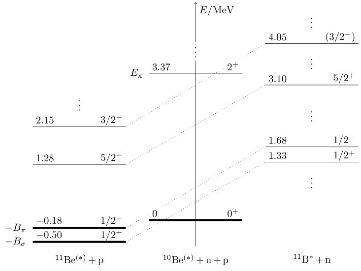 Figure 1
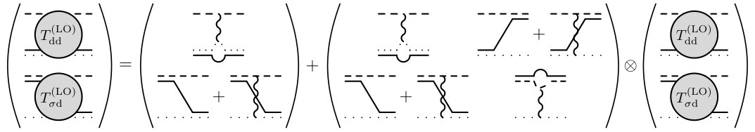 Figure 2
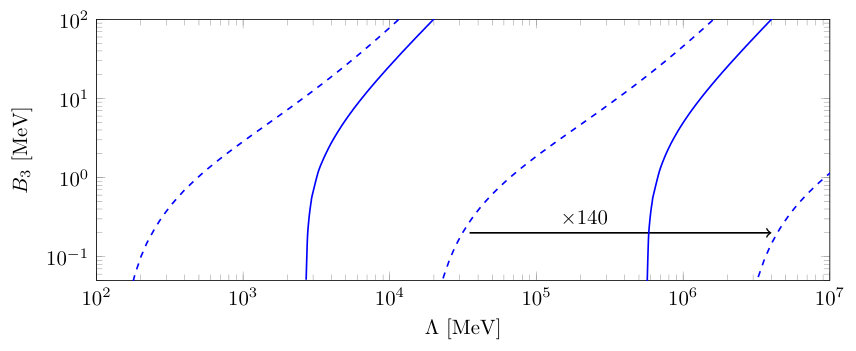 Figure 3
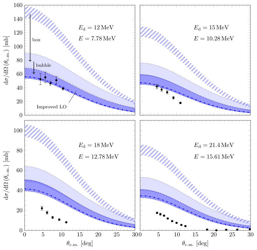 Figure 4
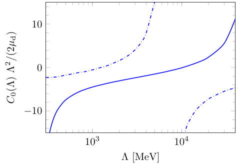 Figure 5
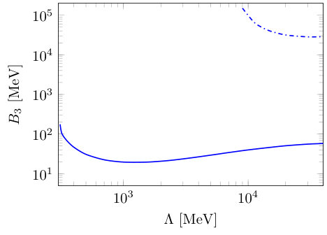 Figure 6
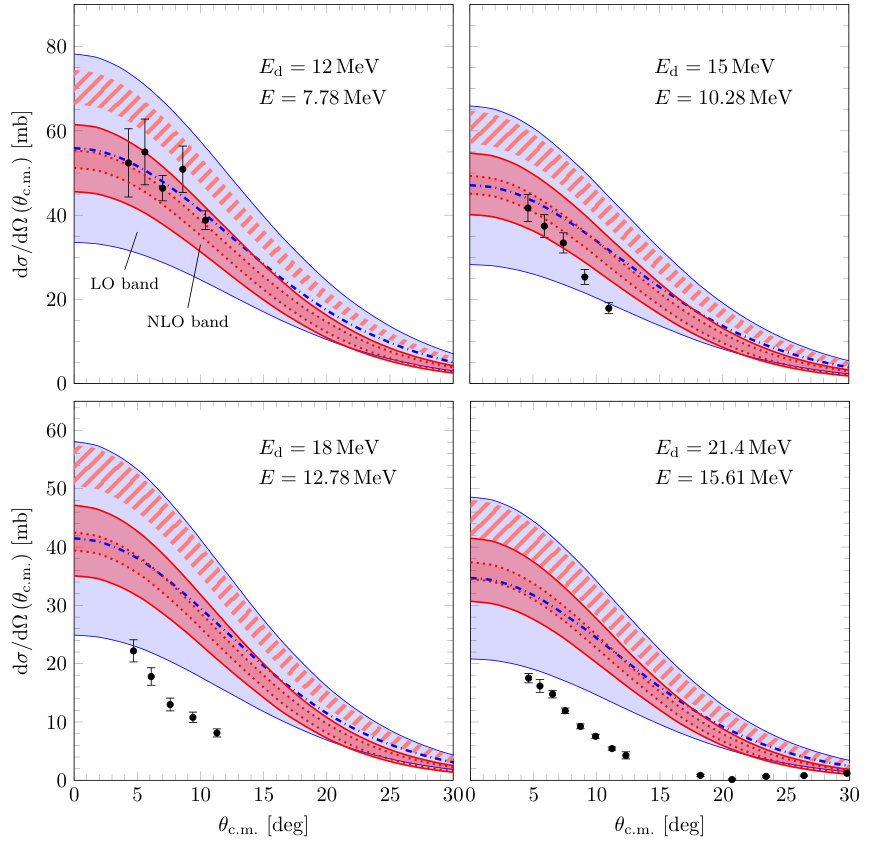 Figure 7
 Figure 8
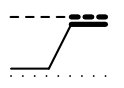 Figure 9
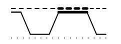 Figure 10
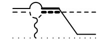 Figure 11
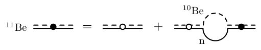 Figure 12
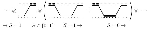 Figure 13
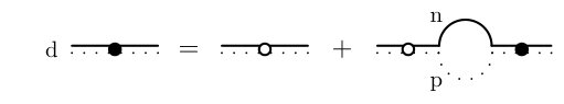 Figure 14
 Figure 15
 Figure 16
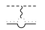 Figure 17
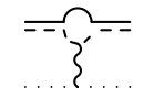 Figure 18
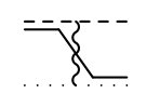 Figure 19
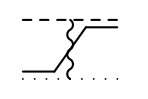 Figure 20
| Subsystem | ||||
|---|---|---|---|---|
| (1) | ||||
| (2a) | ||||
| (2b) |
Peer Reviews
No public reviews on file for this paper yet. If you reviewed it on a platform where reviews are public (OpenReview, ICLR, NeurIPS, ICML), you can paste yours below so the community can read it here.
Videos
No videos yet. Explain this paper in a talk, walkthrough, or lecture? Add one.
Neutron transfer reactions in halo effective field theory
M. Schmidt
Institut für Kernphysik, Technische Universität Darmstadt, 64289 Darmstadt, Germany
Department of Physics and Astronomy, University of Tennessee, Knoxville, TN 37996, USA
L. Platter
Department of Physics and Astronomy, University of Tennessee, Knoxville, Tennessee 37996, USA
Physics Division, Oak Ridge National Laboratory, Oak Ridge, Tennessee 37831, USA
H.-W. Hammer
Institut für Kernphysik, Technische Universität Darmstadt, 64289 Darmstadt, Germany
ExtreMe Matter Institute EMMI, GSI Helmholtzzentrum für Schwerionenforschung GmbH, 64291 Darmstadt, Germany
(March 15, 2024)
Abstract
Direct reaction experiments provide a powerful tool to probe the structure of neutron-rich nuclei like beryllium-11. We use halo effective field theory to calculate the cross section of the deuteron-induced neutron transfer reaction . The effective theory contains dynamical fields for the beryllium-10 core, the neutron, and the proton. In contrast, the deuteron and the beryllium-11 halo nucleus are generated dynamically from contact interactions using experimental and ab initio input. Breakup contributions are then included by construction. The reaction amplitude is constructed up to next-to-leading order in an expansion in the ratio of the length scales characterizing the core and the halo. The Coulomb repulsion between core and proton is treated perturbatively. Finally, we compare our results to cross-section data and other calculations.
I Introduction
Nuclear processes such as capture and transfer reactions are one focus of ongoing research at existing and forthcoming experimental facilities with radioactive ion beams Fahlander and Jonson (2013). However, the consistent theoretical description of such reactions in ab initio calculations poses significant challenges. Tremendous progress has been made for lighter systems in calculating elastic nucleus-nucleon scattering processes by combining the variational approach of the resonating group model and the no-core shell model in the no-core shell model with continuum P. Navrátil et al. (2016). However, for larger systems it remains a challenging task to calculate reactions in a controlled way and with reliable uncertainty estimates; see for example Refs. Yoshida et al. (2018); Capel et al. (2018); King et al. (2018); F. M. Nunes et al. (2018); Lovell and Nunes (2018).
One alternative approach is to reduce the number of dynamical degrees of freedom. A process can then be described as an effective two- or three-body problem using a Lippmann-Schwinger or Faddeev equation. The remaining challenge is to model the interaction between the degrees of freedom appropriately. A reduction to the minimal degrees of freedom required to obtain a certain observable is frequently the starting point of an effective field theory (EFT) treatment of a system. EFTs can be applied if a system displays two disparate scales that can be combined to form a small expansion parameter. The large scale can for example be the excitation energy of a degree of freedom or a heavy state not included in the approach. EFT is the theory in which these high energy modes are integrated out.
Halo nuclei display such a separation of scales M. V. Zhukov et al. (1993); Hansen et al. (1995); Jonson (2004); Jensen et al. (2004). They consist of a tightly bound core with large excitation energy and some weakly bound valence nucleons. The EFT that has been developed for these systems is called halo effective field theory (Halo EFT) Bertulani et al. (2002); Bedaque et al. (2003a). It treats the core as a fundamental degree of freedom, which is a valid approximation as long as energies smaller than are considered. Halo EFT has been applied to a variety of processes including electromagnetic transitions and Coulomb dissociation of one-neutron halo nuclei. The formalism has been extended to one-proton and two-neutron halo nuclei. For a recent review, see Ref. Hammer et al. (2017).
In this work, we explore the potential of Halo EFT to describe the experimentally important process of a deuteron-induced transfer reaction. Such a calculation has not been carried out yet due to the challenging continuum structure of the reaction. As a test case, we consider . The effective three-body system is given by a core, a neutron, and a proton. The one-neutron halo nucleus represents a neutron-core state with a binding energy much smaller than the core excitation energy ; see Fig. 1. This intrinsic scale separation reflects itself also in the small core radius and the large halo radius W. Nörtershäuser et al. (2009). Exploiting these length scales, we construct the reaction cross section at leading order (LO) and next-to-leading order (NLO) in . We find that dynamical core excitations and strong proton-core interactions can be neglected up to NLO. Deuteron and breakup contributions will be included automatically since Halo EFT contains all continuum states of the active degrees of freedom (core, proton, and neutron).
We expect that the Halo EFT expansion works best for center-of-mass energies well below ; see Fig. 1. However, in the absence of appropriate data, we compare our theory to data at , measured by Schmitt et al. at Oak Ridge National Laboratory K. T. Schmitt et al. (2012); Schmitt et al. (2013). In fact, previous works suggest that Halo EFT could still be appropriate for the lower experimental energies. For example, Deltuva et al. calculated the differential cross section in a Faddeev approach, using model interactions that reproduce elastic proton-core scattering data and optical potentials that account for loss channels Deltuva et al. (2016). Their work suggests that core excitations barely influence the cross section for . More recently, Yang and Capel Yang and Capel (2018) reanalyzed the reaction by combining the adiabatic distorted wave approximation reaction model with a Halo EFT description of . They found out that, for the lower beam energies and forward angles, the reaction is purely peripheral. That is, it only depends on the asymptotic form of the wave function, while being independent of short-range details. Indeed, we will be able to describe data for the lower beam energies.
This manuscript is structured as follows. In Sec. II, we present the EFT Lagrangian. Strong interactions among the core, neutron, and proton are described by contact forces and the Coulomb interaction follows from photon couplings. Section III explains how the two-body states , and the deuteron emerge dynamically from the given interactions. We then turn to the three-body system in Sec. IV. A Faddeev equation for the reaction will be constructed up to NLO in the expansion. Following work carried out for the three-nucleon sector Rupak and Kong (2003); König et al. (2015), the Faddeev equation will include the dominant Coulomb contributions. After discussing results for the reaction cross section, we summarize our work and give an outlook in Sec. V.
II EFT Lagrangian
The EFT Lagrangian can be written as the sum
[TABLE]
of one-, two-, and three-body interactions and a photon part. The one-body part reads
[TABLE]
It introduces fields , () and for the neutron, proton, and core. They are treated as distinguishable particles. Sums over doubly appearing indices are implicit. Masses are taken to be and .
The photon’s kinetic and gauge fixing terms are given by
[TABLE]
with timelike unit vector . We only consider Coulomb photons, which induce a static potential. The covariant derivative in Eq. (2) with charge operator induces respective photon couplings with and . As done in Ref. König et al. (2016), we introduce a screened Coulomb photon propagator
[TABLE]
The artificial photon mass has to be taken to zero at the end of each calculation.
The two-body part involves the auxiliary fields () and () for the shallow bound states and deuteron, respectively. It reads
[TABLE]
with and a Clebsch-Gordan coefficient . The expression “H.c.” denotes the Hermitian conjugate. The regularization-dependent parameters () will be matched to experiment. Derivatives in Eq. (II) induce range corrections at NLO. The part accounts for further NLO contributions from the first excited state . It is discussed in Appendix D. Higher-order terms in the ellipses are negligible at NLO.
The three-body part contains an -wave deuteron-core interaction which will be used to renormalize the LO reaction amplitude. We write
[TABLE]
III Two-body states
In this section, we show how , , and the deuteron emerge dynamically from contact interactions of the EFT Lagrangian. Our approach automatically takes care of two-body breakup, a crucial ingredient for the transfer reaction due to the small neutron separation energies of deuteron and ; see, for example, Refs. Yilmaz and Gonul (2000); Gomez-Ramos and Moro (2017); A. Di Pietro et al. (2010). Moreover, we explain the effective treatment of core excitation effects in the system.
III.1 The beryllium-11 ground state
In Halo EFT, the ground state () is treated as a pure neutron-core -wave state. Already at LO, its propagator, , depicted as a solid-dashed double line in Fig. 2 (a), contains iterations of the so-called neutron-core self-energy loop to all orders. This important quantity represents a summation over all neutron-core -wave continuum states allowed by energy-momentum conservation. Thus, breakup contributions are automatically included.
As a consequence of the EFT’s Galilean invariance, is a function of the center-of-mass energy only, where denotes the total four-momentum and is the total mass. After resumming the self-energy loop, the propagator111The propagator is diagonal in spin space. Respective factors will be omitted in the following. takes the well-known effective range expansion form
[TABLE]
where is the reduced mass and is the on-shell relative momentum Bethe (1949). In the power divergence subtraction (PDS) scheme with mass scale Kaplan et al. (1998a, b), the scattering length and effective range are connected to the Lagrangian parameters and of Eq. (II) by
[TABLE]
The ellipses in Eq. (7) denote higher-order terms. The unitary cut term is a manifestation of neutron-core continuum contributions.
The propagator has a pole at , or equivalently at , where TUNL Nuclear Data Evaluation Project (a) and are the small binding energy and binding momentum. Thus, Eq. (7) can be rearranged by writing
[TABLE]
where we have expressed in terms of and .
Since the coupling is not an observable, we eliminate it using redefined auxiliary fields ; see, for example, Ref. Grießhammer (2004). Consequently, we have to multiply by and each (neutron-core)- vertex by .
III.1.1 Halo EFT counting and ANC
In Halo EFT, all parameters in Eqs. (7)–(10) scale with certain powers of the large halo radius and the small core radius . The latter represents the natural nuclear physics length scale Hammer and Phillips (2011). We may estimate from the core excitation energy . The EFT expansion parameter is then given by .
As one of the first applications of Halo EFT to electromagnetic processes, Hammer and Phillips used data of the low-energy E1 strength of breakup, to determine a value for Hammer and Phillips (2011). Their result scales like . In contrast, the binding momentum is as small as . It follows that for low momenta , the effective range term in Eq. (10) is of NLO compared to . Higher-order terms in the ellipses are of the order (N3LO) at most Hammer and Phillips (2011).
Once physics in the pole region is reproduced at a desired accuracy, it becomes obsolete to scale the ground-state wave function with a spectroscopic factor. Such scheme dependent quantities are not required in Halo EFT. Instead, Eq. (10) yields an asymptotic normalization coefficient (ANC)
[TABLE]
for the radial wave function , which is fully determined by low-energy observables Hammer and Phillips (2011).
Recently, Calci et al. were able to calculate the ANC using the no-core shell model with continuum A. Calci et al. (2016). Their result was afterward confirmed by Yang and Capel in Ref. Yang and Capel (2018), who extracted the value from the cross-section data of Ref. Schmitt et al. (2013). The value was also confirmed in analyses of breakup at intermediate and high energies in Refs. Capel et al. (2018); Moschini and Capel (2019). We will use the ANC of Calci et al. as an input parameter at NLO. Equation (11) can then be inverted to give a value for the effective range, which reads
[TABLE]
This value is larger than the one obtained by Hammer and Phillips in Ref. Hammer and Phillips (2011). It will still be counted as , since differs by only from .
III.1.2 Propagator expansion
From NLO, the propagator in Eq. (10) exhibits spurious deep poles in addition to the physical one representing Ji et al. (2012). We solve this issue by expanding around in terms of , yielding the series
[TABLE]
The residue of has an analog expansion and reads
[TABLE]
In Sec. IV, will enter the three-body Faddeev equation and is needed to normalize the reaction amplitude. At LO, we will truncate Eqs. (13)–(14) after the leading terms “,” yielding expressions and . The NLO forms and also include the terms linear in . We will follow Bedaque et al. by replacing in the Faddeev kernel at NLO Bedaque et al. (2003b). This straightforward technique is often referred to as “partial resummation,” because it induces specific amplitude terms proportional to , . In principle, such terms only occur at higher orders. However, for natural cutoffs, they are smaller then NLO terms and do not undermine the validity of the NLO calculation Ji et al. (2012); Ji and Phillips (2013).
III.1.3 Core excitation effects
So far, we have treated as a pure neutron-core state. However, in principle, it also couples to the configuration of a neutron and a core excitation ( wave). Note that this threshold resides far above the pole at an energy separation ; see Fig. 1. Close to the pole, is insensitive to nonanalyticities of this remote channel.
Instead, it only receives residual modifications, which are automatically taken into account by renormalization onto low-energy observables , , etc. Indeed, Deltuva et al. confirmed that dynamical core excitations within the bound state barely influence the reaction cross section Deltuva et al. (2016). In other words, our effective single-channel description readily contains all the relevant core excitation information in the pole regime. For illustration, we show in Appendix A that our approach is equivalent to a theory with an explicit field.
III.2 The beryllium-11 excited state
A second neutron-core state close to threshold is the first excited state (). In Halo EFT, it is treated as a -wave bound state Hammer and Phillips (2011) with binding energy TUNL Nuclear Data Evaluation Project (a), or binding momentum . The Lagrangian part is given in Appendix D. As shown in Ref. Bertulani et al. (2002), shallow -wave states require the inclusion of at least two low-energy parameters. Close to the pole, we choose and the -wave effective range . The propagator expansion then reads
[TABLE]
Similarly to the ground state, can be obtained from the respective ANC Hammer and Phillips (2011). Taking the value of Calci et al. A. Calci et al. (2016), we find
[TABLE]
In the transfer reaction , intermediate states represent NLO corrections to the reaction amplitude since , and higher orders in Eq. (15) are at most of N2LO. For the moment, we neglect the excited state. It will be subject to the NLO discussion in Sec. IV.4.
III.3 The deuteron
The deuteron is treated as an -wave neutron-proton bound state with binding energy de Swart et al. (1995). The product of the small binding momentum and the effective range de Swart et al. (1995) is as small as . It follows that, up to NLO (), the deuteron propagator can be obtained in analogy to the one of . In doing so, one also includes couplings of the deuteron propagator (solid-dotted double line) to the neutron-proton -wave continuum; see Fig. 2 (b).
After performing field redefinitions , expressions for the propagator222The deuteron propagator is diagonal in spin space, i.e., it has to be multiplied by in diagrams. around the pole, its residue , and respective truncations can be obtained from Eqs. (13)–(14) by replacing all subscripts “” by “”, the total mass by , and the reduced mass by . Relativistic effects and - mixing are negligible up to NLO as shown by Chen et al. Chen et al. (1999).
III.4 Other partial wave channels
Two-body interactions in partial waves different from the ones discussed above are negligible at NLO. For example, the virtual state of neutron-proton scattering enters the reaction at N2LO. Neutron-proton -wave interactions enter at N3LO due to the lack of shallow states. Strong proton-core resonances shown in Fig. 1 would also enter at N3LO. Details on how to obtain these power counting classifications in Halo EFT will be given at the end of Sec. IV.4.
Even though two-body interactions are restricted to channels with shallow states, the free (noninteracting) two-body continua will be taken care of in all partial wave channels; see below. These channels are described by plane waves up to NLO.
IV Three-body system
In this section, we derive an integral integration for the reaction cross section from interactions of the Lagrangian up to NLO in the expansion. First, we show which strong and Coulomb diagrams are induced by couplings of the Lagrangian . Second, we construct the LO transfer amplitude and present results for the LO cross section. At the end of the section, we discuss NLO corrections.
IV.1 Power counting and LO diagrams
The transfer amplitude connects the two states
[TABLE]
through neutron exchanges and Coulomb diagrams. In EFT, these diagrams can be classified in a systematic power counting, which exploits the typical momentum scales of the system.
IV.1.1 Momentum scales
The typical momentum scales of the three-body system are given by the small binding momentum scale and the inverse core radius . The largest subleading corrections in the strong sector are suppressed by ; see above.
Coulomb diagrams additionally introduce the small “Coulomb momentum”
[TABLE]
where is the fine structure constant. Moreover, Rupak and Kong pointed out that external momenta have to be counted separately from in the presence of Coulomb photons Rupak and Kong (2003). In this work, we calculate cross sections for center-of-mass energies . Thus, is of the order . The two scales and form a second expansion parameter , which we will count like .
IV.1.2 Strong interaction
In Fig. 3, we display the neutron exchange diagrams that form the elementary building blocks of the strong interaction part of the transfer amplitude. We denote them by and , where and represent total incoming and outgoing spins and their projections, respectively.
Let () be the incoming (outgoing) relative momentum333In this work, relative momenta in the three-body center-of-mass system are defined as the momentum of the respective spectator particle. That is, they equal in , or in . and the center-of-mass energy. We then find
[TABLE]
where is the mass ratio. Due to the -wave nature of the short-range interactions, only transitions between spin states with projections are possible. In the following, we will refer to the functions in Eqs. (19)–(20) as “neutron exchange potentials”.
For neutron exchanges, we use the standard power counting of pionless EFT, which counts all momenta formally like . Loops, one-body propagators, and -wave two-body propagators then count like , , and , respectively. It follows that all neutron exchange iterations are of order and have to be resummed at LO.
Recall that we include deuteron and breakup within the two-body-state propagators (double lines) to all orders by coupling them to continuum states as shown in Fig. 2. In three-body diagrams, further breakup contributions occur. For example, consider the diagram in Fig. 3 (a). The first444Time flows from left to right in our diagrams. (upper) vertex in this diagram describes the breakup of the incoming bound state into a neutron-core pair. At this point, the initial state evolves into an interacting three-body state. Afterward, the exchanged neutron combines with the proton into a deuteron. Physically, the intermediate three-body state can be on shell since the center-of-mass energy is positive in the experiment by Schmitt et al. K. T. Schmitt et al. (2012); Schmitt et al. (2013). Correspondingly, Eq. (19) exhibits poles for .
IV.1.3 Coulomb contributions
Next, we consider the Coulomb force, whose repulsion is expected to lower the reaction probability. In calculations, it is usually included as a static two-body potential in addition to some nuclear model interaction. In a strict EFT approach, however, Coulomb diagrams can be analyzed in a systematic power counting, which exploits the system’s momentum scales. This procedure reveals the relative importance of neutron exchange and Coulomb diagram interactions.
Photon couplings in induce the diagrams () in Fig. 4. Their mathematical expressions are given in Appendix C. In the following, we analyze the diagrams using the Coulomb power counting suggested by Rupak and Kong Rupak and Kong (2003).
Bubble diagrams
The one-loop diagrams (a) and (b) in Fig. 4 are proportional to the photon propagator () and to ; see Eq. (18). All momenta in the loop (“bubble”) may be counted like . 555This statement can be verified by analyzing the bubble diagrams in the limit of zero momentum transfer, where they are largest; see Appendix C. That is, we count one-body propagators like and the loop integration by . The resulting scaling suggests that bubble diagrams are small compared to neutron exchanges () since .
Box diagrams
In the box diagrams of Figs. 4(c) and 4(d), the photon is part of a loop. In this case, it is not straightforward to see if the corresponding integral is governed by powers of or . Since in our case, the safest option is to count the loop like . This scheme is in line with Ref. König et al. (2015). The overall scaling implies that box diagrams are of the same order as neutron exchanges since .
In summary, the Rupak and Kong counting suggests that box diagrams should be iterated at LO, while bubble diagrams are subleading (). However, one important feature of the bubble diagrams is not captured by the counting. Their photon propagators exhibit infrared divergences at small momentum transfers in the limit of vanishing photon mass; see Eqs. (43)–(44). In principle, this enhancement could compensate for the discussed suppression. We account for this possibility by including the bubble diagrams already in the LO calculation, as was also done in Ref. König et al. (2015). We will then critically assess this choice by comparing the numerical influence of the box and bubble diagrams on the cross section.
Note that we only consider diagrams with one photon exchange between two strong interactions. Corrections from two or more successive exchanges should be small since they involve further powers of the small Coulomb momentum . In principle, they could be included by replacing each photon propagator with the full Coulomb matrix; see for example König et al. (2015). We have checked that, for example, would be modified by around in the on-shell limit. Such effects are neglected in this work.
IV.2 Transfer amplitude at LO
By iterating neutron exchanges, Coulomb bubble diagrams, and Coulomb box diagrams to all orders, we obtain the LO transfer amplitude . The corresponding Faddeev equation (without three-body force) is shown diagrammatically in Fig. 5. Loop integrals on the right-hand side ensure that all intermediate states allowed by energy-momentum conservation are taken care of.
IV.2.1 Partial wave channels
It is beneficial for our purposes to perform a partial wave projection onto the total angular momentum with total spin and total orbital angular momentum . This procedure is explained in Appendix B. The respective neutron exchange potentials
[TABLE]
depend on Legendre functions of the second kind,
[TABLE]
in the convention of Ref. Abramowitz and Stegun (1964). Unfortunately, partial wave expressions of the Coulomb diagram interactions are impractically lengthy. Instead, we obtain them numerically by calculating
[TABLE]
with .
Cross sections will contain neutron exchange potentials and Coulomb contributions up to some , at which results can be considered converged. It is worth noting that this approach does not only take care of higher partial waves between core-deuteron and proton-. In fact, it automatically includes higher partial waves in each two-body sector (neutron-proton,666For example, when the proton- pair in Fig. 3 (a) is in , then the intermediate three-body state has between the proton and an neutron-core pair. This configuration can be recoupled to between the core and an neutron-proton pair. neutron-core, proton-core) due to breakup within the and diagrams; see Fig. 3. Thus, the free two-particle continua (plane waves) are included up to although interactions are restricted to two-body channels with shallow states.
As indicated in Fig. 5, the LO elastic and transfer amplitudes can be summarized into an amplitude vector . Due to the fact that the total spins and orbital angular momenta are conserved at LO, we identify a specific partial wave system by the superscript “.” For incoming (outgoing) relative momenta (), we finally obtain the scattering equations
[TABLE]
with LO amplitude vector, interaction matrix, and propagator matrix
[TABLE]
and in channel space. For convenience, we introduced the new functions
[TABLE]
where and .
The full transfer amplitude is given as a sum over the partial wave amplitudes and respective projection operators as shown in Appendix B. In all calculations, we truncate the sum at some maximal orbital angular momentum and increase this value toward convergence. Similarly, whenever including Coulomb diagrams, we decrease the photon mass . We find that the cross section converges at and .
IV.2.2 Unphysical deep bound states
To see if Eq. (25) requires a three-body force for renormalization, we have performed an asymptotic analysis for large incoming and loop momenta similar to Ref. Grießhammer (2005). In this limit, nucleon exchanges () dominate over Coulomb contributions () König et al. (2015). Thus, we may neglect the Coulomb force for the moment. It turns out that for , the potentials in Eq. (25) fall off fast enough to produce unique amplitudes solutions. In the system, however, that is not the case. Instead, the amplitudes approach a power law behavior with . It follows that the system exhibits an Efimov effect, i.e., a geometric spectrum of three-body bound states at energies Efimov (1970); Braaten and Hammer (2006); Naidon and Endo (2017). We note that reproduces the universal scaling factor of three distiguishable particles with mass ratio presented in Ref. Braaten and Hammer (2006).
In the following, we equip Eq. (25) with a momentum cutoff . The resulting spectrum is shown in Fig. 6 as dashed lines. Coulomb diagrams do not influence the large momentum behavior of the system qualitatively. They only push the Efimov states to higher cutoffs (solid lines in Fig. 6). The system will be renormalized using the three-body coupling of Eq. (6). It enters the interaction matrix of Eq. (27) as a constant -wave potential like
[TABLE]
Note that the choice of this specific three-body force is not unique. One could also introduce it in the transfer or the elastic channel.
The quantum numbers of the Efimov states correspond to those of a level in boron-12. Experimentally, three such states are known TUNL Nuclear Data Evaluation Project (b). In a deuteron- cluster picture, their binding energies correspond to spatial separations of the deuteron- pair. Being of the order , they do not reflect a separation of scales in the three-body sector. Thus, the cluster picture is not justified and the Efimov states can be understood as artifacts of the short-range approach. However, although unphysical, they do not pose a problem as long as they lie outside the EFT’s region of applicability. Indeed, after renormalization onto cross-section data, all three-body states will occur at binding energies and thus far away from the low-energy region; see Fig. 8 (b).
IV.3 Cross section
The differential cross section of the reaction at a deuteron beam energy
[TABLE]
can be obtained by multiplying the transfer amplitude by the residue factor and evaluating it at on-shell relative momenta,
[TABLE]
The cross section depends on the center-of-mass angle with . In the channel, we set the relative momentum to and in the channel we take . The spin-averaged reaction cross section then reads
[TABLE]
where .
Table 1 summarizes the input parameters needed for the calculation of the reaction cross section up to NLO in the expansion. At LO, only the binding energies and are required. At NLO, also the effective range , the ANC of , and the binding energy and ANC of enter.
IV.3.1 Coulomb suppression and improved LO system
Our first goal is to critically assess the Coulomb power counting performed above. In particular, we would like to validate the proposed LO nature of the Coulomb force in general and of the bubble diagrams specifically, for the experimental energies used by Schmitt et al. K. T. Schmitt et al. (2012); Schmitt et al. (2013). Given the cutoff-dependence of the channel, we vary in the large range in each calculation. This procedure reveals the potential impact of the -wave three-body force on the LO reaction cross sections.
In a first step, we neglect all Coulomb diagrams, which yields the uppermost bands (hatched) in Fig. 7. Each curve is converged at percentage level for . At all four deuteron beam energies (lab frame), the bands lie high above the experimental data by Schmitt et al. K. T. Schmitt et al. (2012); Schmitt et al. (2013). Apparently, the strong interaction alone does not produce enough repulsion between the scattering partners, even if is included.
In order to understand the relative importance of the Coulomb box and bubble diagrams, we add them successively to the Faddeev equation. The light bands surrounded by dotted lines in Fig. 7 show that the box diagrams alone lower the cross sections drastically at all beam energies as expected. Indeed, it is important to include them at LO. Further repulsion comes from the bubble diagrams. Their inclusion yields the dark lowermost bands in Fig. 7. Apparently, the influence of the bubble diagrams on the cross section is smaller than the one of the box diagrams. Thus, it seems as if we have overestimated the enhancement due to the bubble diagrams’ infrared divergences by one order in . A posteriori, the bubble diagrams are of NLO and could in principle be neglected at LO. The “pure LO” system then only contains neutron transfer and box diagrams.
Interestingly, however, the inclusion of the bubble diagrams as one specific NLO correction leads to a surprisingly good agreement with the cross-section data at lower beam energies and forward angles. Thus, choosing the “improved LO” system of Fig. 5 significantly accelerates the EFT convergence. This statement will be verified later by including the remaining NLO corrections. Moreover, the improved LO system, unlike the pure one, can be renormalized onto data at since the respective band comprises all data points. We emphasize that none of the bands in Fig. (7) includes the EFT uncertainties of at LO; see Fig. 9 for comparison.
IV.3.2 Peripherality regions
Although subleading in a strict sense, the bubble diagrams do not introduce any new parameters like, for example, effective range coefficients. Thus, the improved LO system stays independent of short-range details. Cross sections are then only affected by the tail of the wave function, i.e., the reaction is purely “peripheral”. Yang and Capel argued that such a description is sufficient to describe the reaction at lower beam energies and forward angles Yang and Capel (2018). Our results provide clear evidence for this claim since the improved LO band for perfectly describes the whole data region ().
Moreover, according to Yang and Capel, the peripherality region increases (decreases) in size for lower (higher) energies. Indeed, at , only forward scattering () is captured by the improved LO band. Deviations at larger angles are of NLO size. At even higher energies , however, the bands deviate from data by . We conclude that the reaction is indeed only peripheral at forward angles and low energies. For this reason our power counting may fail for energies .
Note, however, that Schmitt et al. identified their data set to be systematically smaller than the other three Schmitt et al. (2013). In particular, they extracted spectroscopic factors from all four data sets, of which the results were smaller. Yang and Capel, who extracted the ANC from the data of Schmitt et al., made a similar observation Yang and Capel (2018). Of all four data sets, only the set yielded an ANC smaller than the prediction by Calci et al. A. Calci et al. (2016). Thus, our calculation might be better at than suggested by Fig. 7.
IV.3.3 Cutoff dependence and renormalizability
Out of all components , only the part is cutoff-dependent. Due to this circumstance, the band widths in Fig. 7 are only the size of the box diagram shift (LO). Such contributions are negligible up to NLO. Thus, in principle, each curve within the filled bands represents an LO result itself and renormalization is not required. Let us emphasize that the only inputs to our LO system are then given by the binding energies and ; see Table 1. At astrophysical energies, however, the component is of much greater importance, leading to a much stronger cutoff dependence.
We demonstrate the renormalizability of the improved LO system using the three-body force . For various cutoffs , we adjust it in a fit to the depicted data set. This procedure yields the two solutions for shown in Fig. 8 (a). Their fit values (solid curve) and (dot-dashed curve) are, within numerical uncertainties, equal in size and respectively constant for . For illustration, we show fit results for in Fig. 7 as dot-dashed curves. The first three-body state occurs at (or ); see Fig. 8 (b). It lies above (or ) and converges to even higher values as .
IV.4 Corrections at NLO and beyond
We now discuss NLO contributions to the reaction cross section in the expansion, stemming from range corrections in the two-body sectors and from the excited state .
IV.4.1 Effective range corrections
A straightforward way to include effective range corrections in the deuteron and is to replace the LO propagators by () in Eq. (25) Bedaque et al. (2003b).777Correspondingly, one has to use the residues in the calculation of the cross section in Eq. (33). This approach reintroduces a cutoff dependence in the channel. In principle, it could be cured by readjusting the three-body force Hammer and Mehen (2001). In order to see the impact of the additional cutoff dependence, we include effective range corrections in the renormalized improved LO system for various . 888Below , the renormalized improved LO result is not yet converged. Note that the cutoff variation up to is only used to estimate higher-order corrections. It does, however, not reveal the necessity of additional counter terms. Figure 9 shows that the resulting red hatched bands lie well within the LO uncertainty bands (blue, enclosed by thin solid lines) of the improved LO estimates (blue dot-dashed curves). The band widths are comparably small, giving rise to a mild cutoff dependence.
It has to be mentioned that a small fraction of the band widths stems from an unexpected cutoff dependence in the sector. It can be understood as an artifact of the choice, not to perturb the amplitude itself to first order in , but the integration kernel. That modifies the UV behavior of the partial wave amplitudes, leading to a divergence in the sector. This divergence would not be present in a strictly perturbative approach Grießhammer (2005). Even though desirable, such a more involved NLO treatment lies beyond the scope of this work. In fact, we have checked that the influence of the cutoff on the amplitude is less than over the range . Thus, this issue can be neglected at NLO.
IV.4.2 The beryllium-11 excited state
The excited state introduces a third channel to the three-body system. It couples to via the diagrams shown in Figs. 10(a) and 10(b). Their mathematical forms and partial wave projections are given in Appendix D. We note that only occurs as an intermediate state in the reaction. Thus, the NLO nature of follows from the propagator scaling ; see Sec. III. A typical contribution to the reaction amplitude is given by Fig. 10(c). Again, we count all loop momenta like . The two (neutron-core)- vertices contribute a factor . The overall scaling is then one order smaller than the LO scaling .
We complete the NLO system by inserting both effective range corrections in and , and the potentials into the integration kernel. The resulting Faddeev equations are given in Appendix E. Similarly to the previous calculation, we vary and include the LO three-body force . Figure 9 shows that the results of the previous calculation (hatched bands) get shifted back toward the improved LO results, ending up as red bands enclosed by dotted lines. Thus, the influence of is indeed of NLO, in agreement with our power counting. The remaining cutoff dependencies of the and sectors are negligible compared to N2LO corrections (, red uncertainty bands enclosed by thick solid lines). Thus, no further renormalization is needed at NLO.
Recall that the NLO parameters and were calculated in Eqs. (12) and (16) from the ANCs of Calci et al. A. Calci et al. (2016). Instead, one could directly use the Halo EFT values and of Hammer and Phillips Hammer and Phillips (2011). The relative differences and are of size and should thus be negligible at NLO. We have checked that the final NLO bands would indeed only change by ca. . Thus, both choices for are consistent with the proposed power counting.
In Ref. Schmitt et al. (2013), the cross section for transfer to was also measured. In our theory, this quantity can in principle be calculated using the amplitudes in Eqs. (60)-(61). However, Yang and Capel found that this process is less peripheral than Yang and Capel (2018). For this reason, we expect that our low-energy power counting has to be modified in order to describe it. Indeed, naive application of the current scheme leads to an overestimation of the data.
IV.4.3 Higher-order interactions
At higher orders in Halo EFT, additional interactions would enter the calculation. For example, the proton-neutron sector exhibits a shallow virtual state Kaplan et al. (1998a, b). It does not occur at LO, because the total neutron-proton spin is conserved if all interactions are of -wave type. In the presence of the -wave state , however, may change, and transitions become possible; see Fig. 11. However, the virtual state is not only suppressed due to the intermediate channel. Since multiple spin changes [ or smaller] are negligible at NLO, a virtual state leads to in the final state of . The corresponding phase space is the size of , yielding a suppression of (N2LO).
Neutron-proton -wave interactions are of order N3LO. The reason is the lack of a shallow neutron-proton -wave bound or resonance state. In the sector, approaches the large scattering volume for small Typel and Baur (2004). This large value is a consequence of the small binding momentum since ; see Eq. (15). Scattering volumes in the neutron-proton channels , , , and are much smaller. Using the Nijmegen partial wave analysis for N-N scattering of Ref. Stoks et al. (1994), we have checked that they are all of the natural size or smaller (N3LO). In fact, the -wave phase shifts themselves are suppressed compared to the phase shift. Even for the maximal neutron-proton center-of-mass energy available in the experiment by Schmitt et al., the suppression is of the order (N3LO).
In Ref. Goosman et al. (1970), several boron-11 resonances have been observed in ; see Fig. 1. The lowest one () occurs at a proton-core center-of-mass energy . It has a total width and the branching ratio for decay into is close to Goosman et al. (1970). The resonance represents a pole at in the Coulomb-modified resonance propagator; see for example Refs. Kok et al. (1982); Kong and Ravndal (1999a). This pole position implies effective range terms and , which scale like . Moreover, in three-body diagrams, the resonance propagator comes along with a Gamow-Sommerfeld factor Kong and Ravndal (1999b). It gives the probability of two charged particles to meet in one point. At resonance, it takes the small value . It follows that the influence of the resonance propagator on the reaction is suppressed by three orders in compared to (N3LO). Note that there are more boron-11 states around , which could possibly couple strongly to the proton-core system. However, transitions to those states would involve even smaller Gamow factors . Thus, we neglect strong proton-core interactions at NLO.
During the reaction process, the state could break up into an excited core and a neutron. Thus, in principle couples to the additional intermediate channel via neutron exchanges. However, each such channel comes along with two couplings of order ; see Appendix A for details. Thus, dynamical core excitations can be neglected at NLO.
Diagrams involving direct photon couplings to the auxiliary fields and do not enter before N2LO. They are one order smaller than the bubble diagrams König et al. (2016), which are de facto of NLO; see above. The Coulomb field could also induce E transitions between and (or between the deuteron and a neutron-proton -wave channel) Hammer and Phillips (2011). Such a contribution is shown in Fig. 10 (d). It is negligible at NLO due to the subleading nature of the propagator and due to the photon propagator, which is governed by the large external momentum scale .
V Summary and outlook
In this work, we carried out the first Halo EFT calculation of deuteron-induced transfer reactions. As a working example, we considered , involving the one-neutron halo nucleus . The degrees of freedom in this approach are the core, the neutron, and the proton. Strong interactions are described by contact forces alone. To obtain the differential cross section, the reaction amplitude was constructed diagrammatically in an expansion in the ratio of core and halo radius. The corresponding Faddeev equation contains all dynamical features of a transfer reaction including two-body breakup contributions. A three-body force ensures internal consistency. We included the Coulomb force by considering the dominant photon exchange diagrams, which were iterated to all orders in the Faddeev equation.
The differential cross section was compared to experimental data by Schmitt et al. K. T. Schmitt et al. (2012); Schmitt et al. (2013). In agreement with Yang and Capel Yang and Capel (2018), who calculated the cross section in the adiabatic distorted wave approximation, we found that Halo EFT is able to describe scattering at low beam energies (center-of-mass energies ). In this regime, the reaction can be considered peripheral, i.e., it predominantly depends on the long-range tail of the wave function. This part is systematically reproduced by the expansion.
Our theory contains only few information on the spectra of the involved particles. We included, in particular, only two-body states with a binding momentum clearly smaller than the respective momentum scale of short-range physics; see Fig. 1. The influence of such states should be enhanced by powers of compared to those far away from the two-body threshold. As a consequence of this reduction, we were able to describe data using only a minimal amount of experimental input. At LO in the expansion, only the binding energies of deuteron and are needed; see Table 1. NLO corrections arise from respective effective ranges and the first exited state . The effective ranges of the states were extracted from the ANCs of the ab initio calculation by Calci et al. A. Calci et al. (2016). Both NLO corrections modify the cross section at a level, as predicted by the power counting.
While our results describe data at fairly well, they strongly overestimate the cross section at higher beam energies. Apparently, the low-energy expansion of Halo EFT converges, if at all, slowly at these energies. In order to improve the expansion, it might be necessary to modify the three-body power counting, which, at the moment, counts loop momenta like small binding momenta. In a more sophisticated power counting, tailored to beam energies , neglected higher-order interactions might already occur at lower orders. Such a scheme should be developed in the future. Hints on missing ingredients can be inferred from previous theoretical analyses, e.g., by Schmitt et al. in Ref. Schmitt et al. (2013), Deltuva et al. in Ref. Deltuva et al. (2016), or Yang and Capel in Ref. Yang and Capel (2018), which were successful in describing also scattering for . The model used in Ref. Yang and Capel (2018) contains the same amount of information on the spectrum as our work. Thus, we do not expect the inclusion of beryllium-11 levels beyond the first excited state to be of prime importance.
Instead, core excitations following breakup and two-body interactions in higher partial waves might provide enough absorption to lower cross sections at higher energies. Moreover, we might need to consider not explicitly measured loss channels, in particular due to deep boron-11 states indicated in Fig. 1, at these energies. Usually, such effects are included using optical model potentials, adjusted to, for example, proton-core scattering data. In the future, we will instead introduce imaginary contact terms to the strong Lagrangian, a method called “Open EFT” Braaten et al. (2016). It was applied successfully to a broad range of inelastic processes including quarkonium decays in nonrelativistic QCD Bodwin et al. (1995) and three-body recombinations of ultracold atoms Braaten and Hammer (2001).
Let us emphasize again, that Halo EFT is ideally suited for the description of strong interactions at low energies. In this sense, our long-term goal is to apply the developed framework to the astrophysical regime. While Coulomb effects become nonperturbative then, short-range effects should become less important. In this context, it will be interesting to calculate the cross section for ∗, which was measured in by Schmitt et al. K. T. Schmitt et al. (2012); Schmitt et al. (2013). This process is less peripheral than Yang and Capel (2018), which is why naive application of the current power counting at experimental energies leads to an overestimation of the data. At very small energies, however, the power counting should be appropriate. Note, however, that certain Coulomb diagrams involving , which we could neglect for , would become important for ∗. Moreover, we could apply the framework to other deuteron-induced reactions like .
Acknowledgements.
We thank D. R. Phillips for giving valuable feedback on the manuscript and S. König for providing information on the calculation of the Coulomb box diagrams. M. S. appreciates stimulating discussions with I. Thompson, D. Baye, and other participants of the INT Program INT-17-1a “Toward Predictive Theories of Nuclear Reactions Across the Isotopic Chart.” Moreover, M. S. sincerely thanks the Nuclear Theory groups of UT Knoxville and Oak Ridge National Laboratory for their kind hospitality and support during his research stay. This work has been funded by the Deutsche Forschungsgemeinschaft (DFG, German Research Foundation), Projektnummer 279384907, SFB 1245, by the National Science Foundation under Grant No. PHY-1555030, by the Bundesministerium für Bildung und Forschung (BMBF) through Contract No. 05P18RDFN1, and by the Office of Nuclear Physics, U.S. Department of Energy under Contract No. DE-AC05-00OR22725.
Appendix A Core excitation effects
In this section, we show that core excitation effects in the pole region are taken care of in this work due to renormalization onto low-energy observables. For that, we consider a theory with an explicit field () by adding a piece
[TABLE]
to the Lagrangian. A similar approach has been chosen by Zhang et al. to analyze effects of the core excitation on the reaction Zhang et al. (2014a). Moreover, Zhang et al. and Ryberg et al. used a core excitation field in their calculations of the -factor of Zhang et al. (2014b); Ryberg et al. (2014). In both systems, the core excitation occurs at low energies. That, however, is not true in our case where is large.
Together with a neutron, couples to the ground state in a -wave. In terms of the redefined field , we thus write
[TABLE]
The vertex term contains a Galilei-invariant derivative . It is embedded in the tensor structure
[TABLE]
with , where denotes a spherical harmonic, evaluated at .
The mass difference in the transition is of natural size. Thus, we assume no fine-tuning in this scattering channel and count . It follows that the overall couplings are natural as well, since ; see Eq. (9).
The core excitation modifies the propagator through the -neutron self-energy loop . It resembles the -neutron self-energy loop of Fig. 2, but the core line has to be replaced by a core excitation line. Using the PDS scheme, we find
[TABLE]
Note that is analytic for , i.e., it can be expanded at . The resulting coefficients then contribute to the unrenormalized parameters () of the bare propagator; see Eq. (II). Thus, renormalization onto observables (or ), , etc. automatically takes care of core excitation effects at small , where the pole is located. In other words, does not introduce any new information to the two-body sector and can be integrated out.
Appendix B Partial wave expansion
Let us consider a general interaction , which could be an amplitude , a neutron exchange potential or a Coulomb diagram interaction . We expand in tensor spherical harmonics
[TABLE]
by writing
[TABLE]
Specific partial waves can be extracted via
[TABLE]
Appendix C Coulomb diagrams
The Coulomb diagrams in Fig. 4 resemble such considered by König et al. for the three-nucleon system König et al. (2016). However, they exhibit nontrivial dependencies on the mass ratio . The bubble interactions read
[TABLE]
and the box interactions are given by
[TABLE]
where we defined . Moreover, is the fine structure constant and is the core charge. All interactions involve the function
[TABLE]
whose arguments involve the expressions
[TABLE]
The form of can be simplified significantly by neglecting terms of order ; see Eq. (44). This approximation is justified since is a tiny number. The only angular dependence then comes from the photon propagator, which can be projected onto certain partial waves analytically.
The bubble diagrams and are linear in the Coulomb propagator. Thus, their largest contributions to the transfer reaction comes from the region of small momentum transfers . For , the values of the function in Eqs. (43)–(44) collapse to (). Thus, the deuteron and halo loops of the LO bubble diagrams in Fig. 4 may be counted like .
The Coulomb diagram interactions can be connected to the -wave projected functions and of Ref. König et al. (2016) by taking the limits . We find
[TABLE]
where .
Appendix D Excited state of beryllium-11
In this section, we discuss the inclusion of the excited state at NLO in the reaction calculation. The Lagrangian part
[TABLE]
of Eq. (II) contains an auxiliary field () for with renormalization-dependent parameters . The Galilei-invariant derivative and the -wave tensor structure are defined in Appendix A. Unlike in the -wave case, both the constant and derivative part of the bare propagator term in Eq. (52) are needed to describe the shallow -wave state Bertulani et al. (2002); Hammer and Phillips (2011). The full propagator can be obtained by resumming all two-body loops, similarly to Fig. 2. For more details, we refer to Ref. Hammer and Phillips (2011). After proper renormalization and field redefinitions , the propagator around the pole at is given by Eq. (15).
In the NLO three-body system, the intermediate state couples to via neutron exchange potentials shown in Fig. 10. They read
[TABLE]
with in the channel and involve a symbol. Partial wave projections are given by
[TABLE]
A direct transition potential between and is not induced by the Lagrangian, i.e., these states can only be connected via an intermediate state .
The Clebsch-Gordan coefficient and the symbols in Eq. (55) imply some selection rules. First, only transitions with are allowed. It follows that for , we have , and for fixed , the system decouples into the two subsystems (1) and (2) . Second, is fixed in subsystem (1), while both options are allowed in subsystem (2). Last, in subsystem (2), the two channels further decouple after defining rotated spin states
[TABLE]
Note that and for . The corresponding partial wave potentials read
[TABLE]
In summary, for fixed , we find the three decoupled subsystems (1), (2a), and (2b) presented in Table 2. Just as in the LO case, they can be identified by the conserved quantum number (1) , (2a) , and (2b) . In the case , only system (2b) is allowed.
Appendix E NLO equations
As explained in Appendix D, the introduction of the excited state produces three decoupled scattering systems for fixed , corresponding to , and a single system for with . The respective NLO amplitude vectors read
[TABLE]
They are determined by the interaction and propagator matrices
[TABLE]
and
[TABLE]
respectively, similar to Eq. (25). The propagator function is defined via Eq. (29) with and reduced mass .
The reference list from the paper itself. Each links out to its DOI / PubMed record.
- 1Fahlander and Jonson (2013) C. Fahlander and B. Jonson, Phys. Scripta T 152 , 010301 (2013).
- 2P. Navrátil et al. (2016) P. Navrátil et al. , Phys. Scripta 91 , 053002 (2016), eprint 1601.03765.
- 3Yoshida et al. (2018) K. Yoshida, M. Gómez-Ramos, K. Ogata, and A. M. Moro, Phys. Rev. C 97 , 024608 (2018), eprint 1711.04458.
- 4Capel et al. (2018) P. Capel, D. R. Phillips, and H.-W. Hammer, Phys. Rev. C 98 , 034610 (2018), eprint 1806.02712.
- 5King et al. (2018) G. B. King, A. E. Lovell, and F. M. Nunes, Phys. Rev. C 98 , 044623 (2018), eprint 1810.06129.
- 6F. M. Nunes et al. (2018) F. M. Nunes et al. , EPJ Web Conf. 178 , 03001 (2018).
- 7Lovell and Nunes (2018) A. E. Lovell and F. M. Nunes, Phys. Rev. C 97 , 064612 (2018), eprint 1801.06096.
- 8M. V. Zhukov et al. (1993) M. V. Zhukov et al. , Phys. Rept. 231 , 151 (1993).