Asymptotic distribution and convergence rates of stochastic algorithms for entropic optimal transportation between probability measures
Bernard Bercu, J\'er\'emie Bigot

TL;DR
This paper analyzes the convergence and distribution of stochastic algorithms for estimating entropic optimal transportation costs, specifically Sinkhorn divergences, using a Robbins-Monro approach with theoretical guarantees and practical experiments.
Contribution
It establishes almost sure convergence, asymptotic normality, and convergence rates for a new recursive estimator of Sinkhorn divergence in semi-discrete and discrete settings.
Findings
Proves almost sure convergence of the estimator.
Derives asymptotic normality results.
Provides numerical experiments demonstrating effectiveness.
Abstract
This paper is devoted to the stochastic approximation of entropically regularized Wasserstein distances between two probability measures, also known as Sinkhorn divergences. The semi-dual formulation of such regularized optimal transportation problems can be rewritten as a non-strongly concave optimisation problem. It allows to implement a Robbins-Monro stochastic algorithm to estimate the Sinkhorn divergence using a sequence of data sampled from one of the two distributions. Our main contribution is to establish the almost sure convergence and the asymptotic normality of a new recursive estimator of the Sinkhorn divergence between two probability measures in the discrete and semi-discrete settings. We also study the rate of convergence of the expected excess risk of this estimator in the absence of strong concavity of the objective function. Numerical experiments on synthetic and real…
Click any figure to enlarge with its caption.
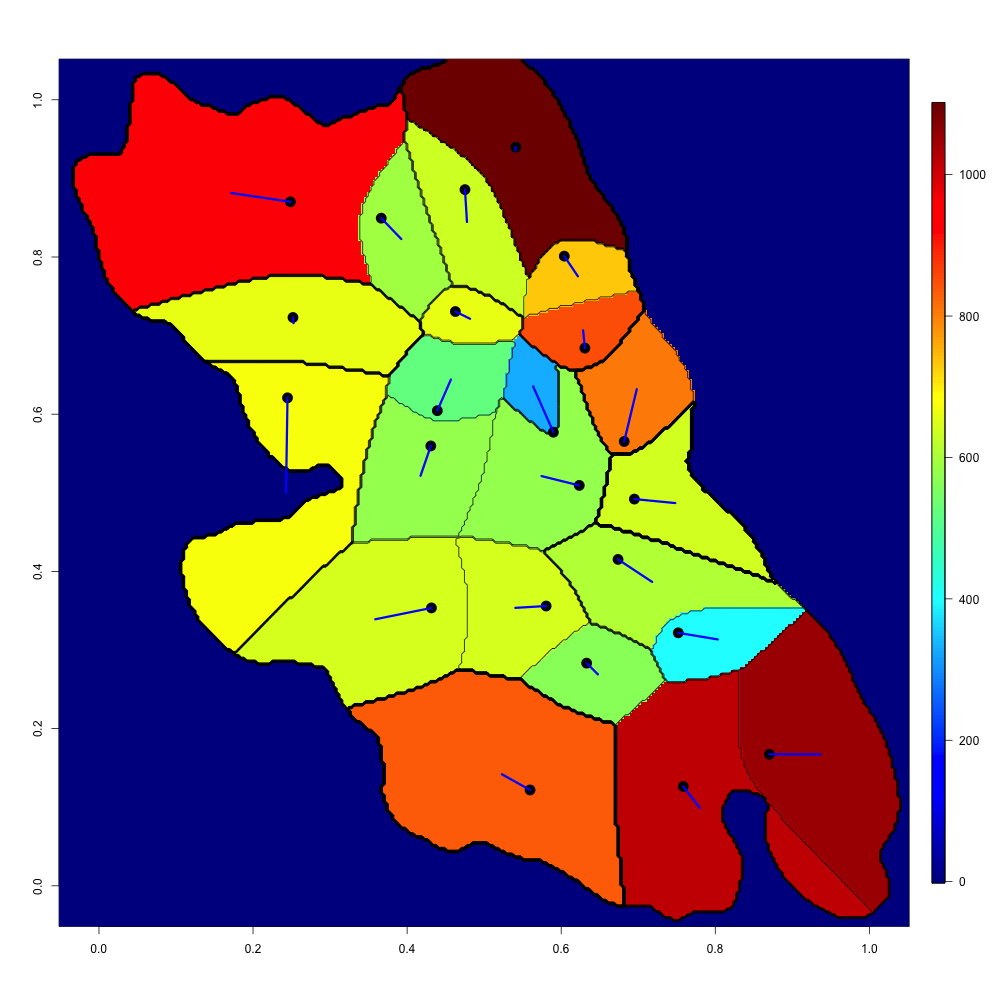 Figure 1
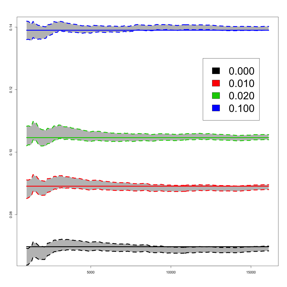 Figure 2
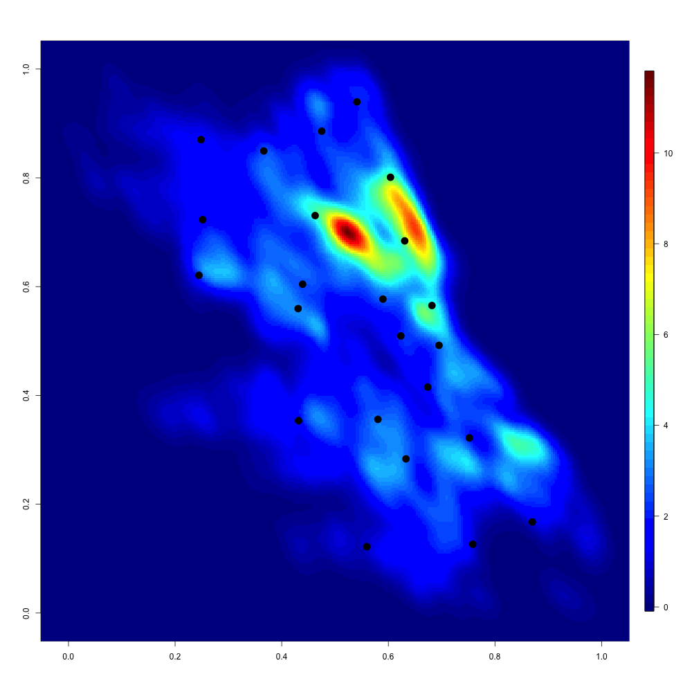 Figure 3
 Figure 4
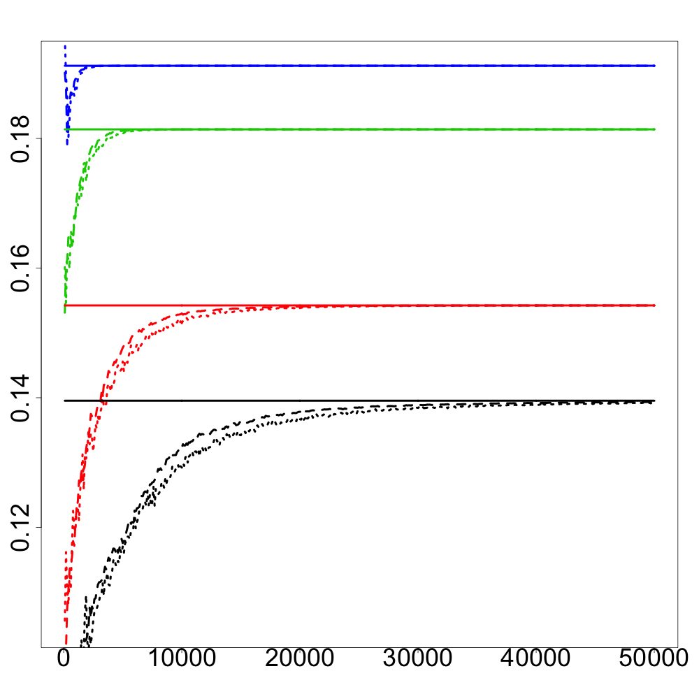 Figure 5
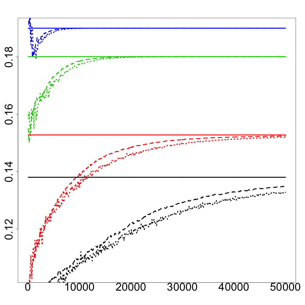 Figure 6
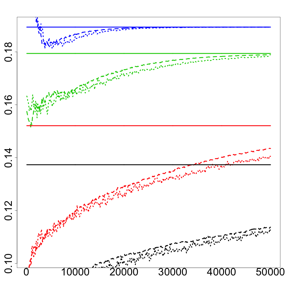 Figure 7
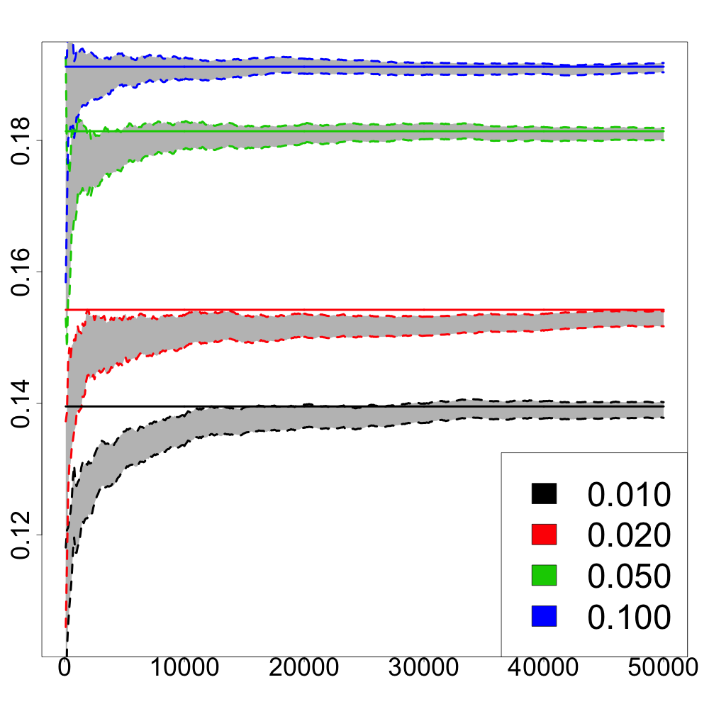 Figure 8
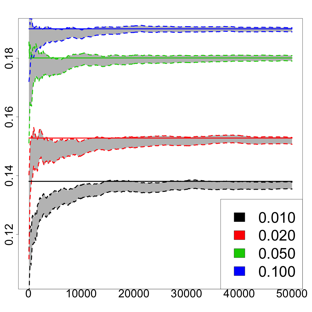 Figure 9
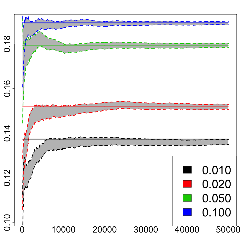 Figure 10
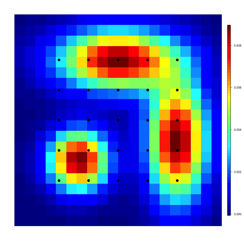 Figure 11
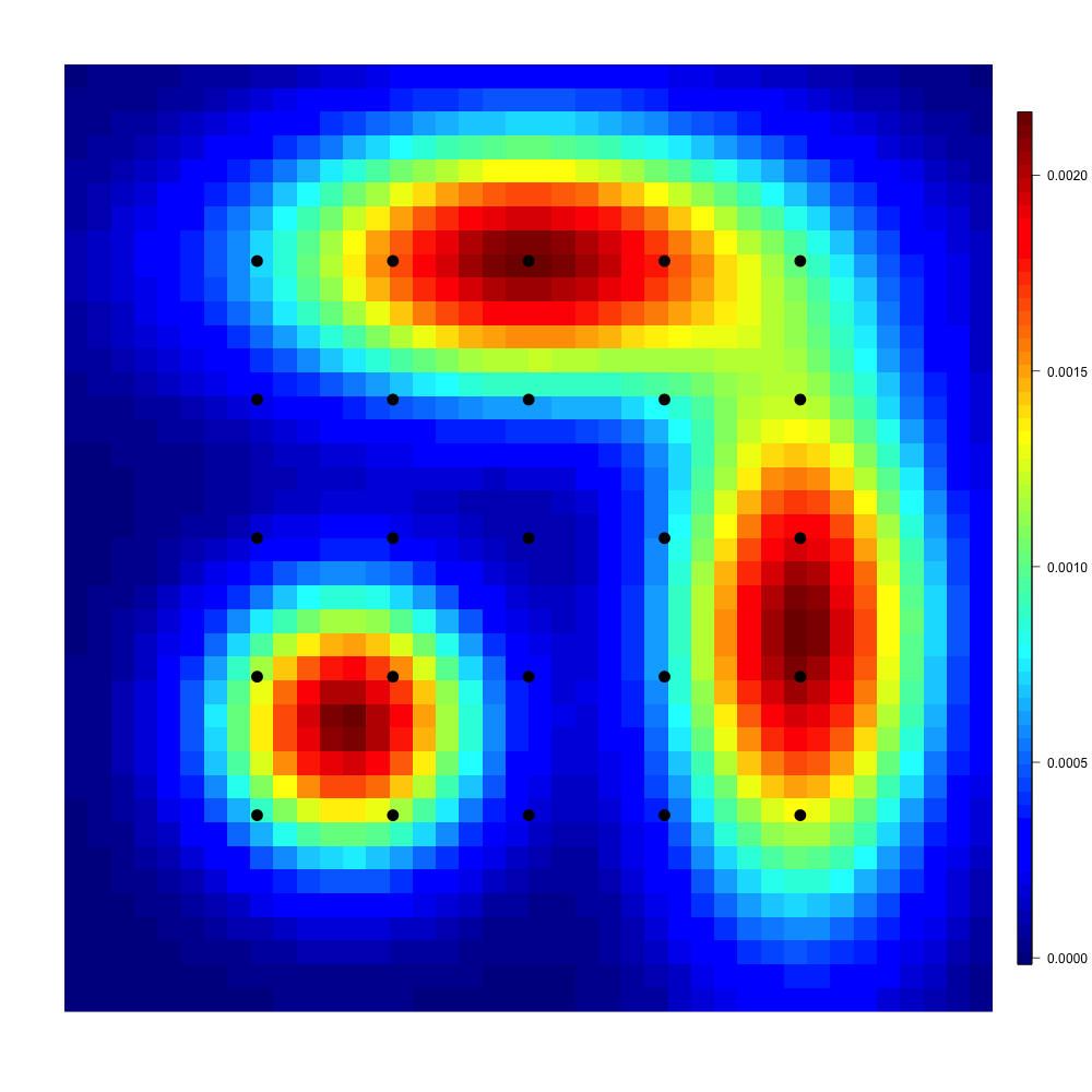 Figure 12
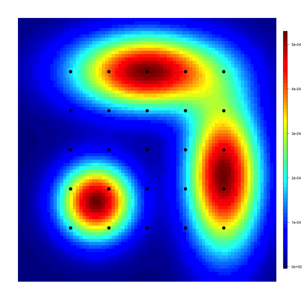 Figure 13
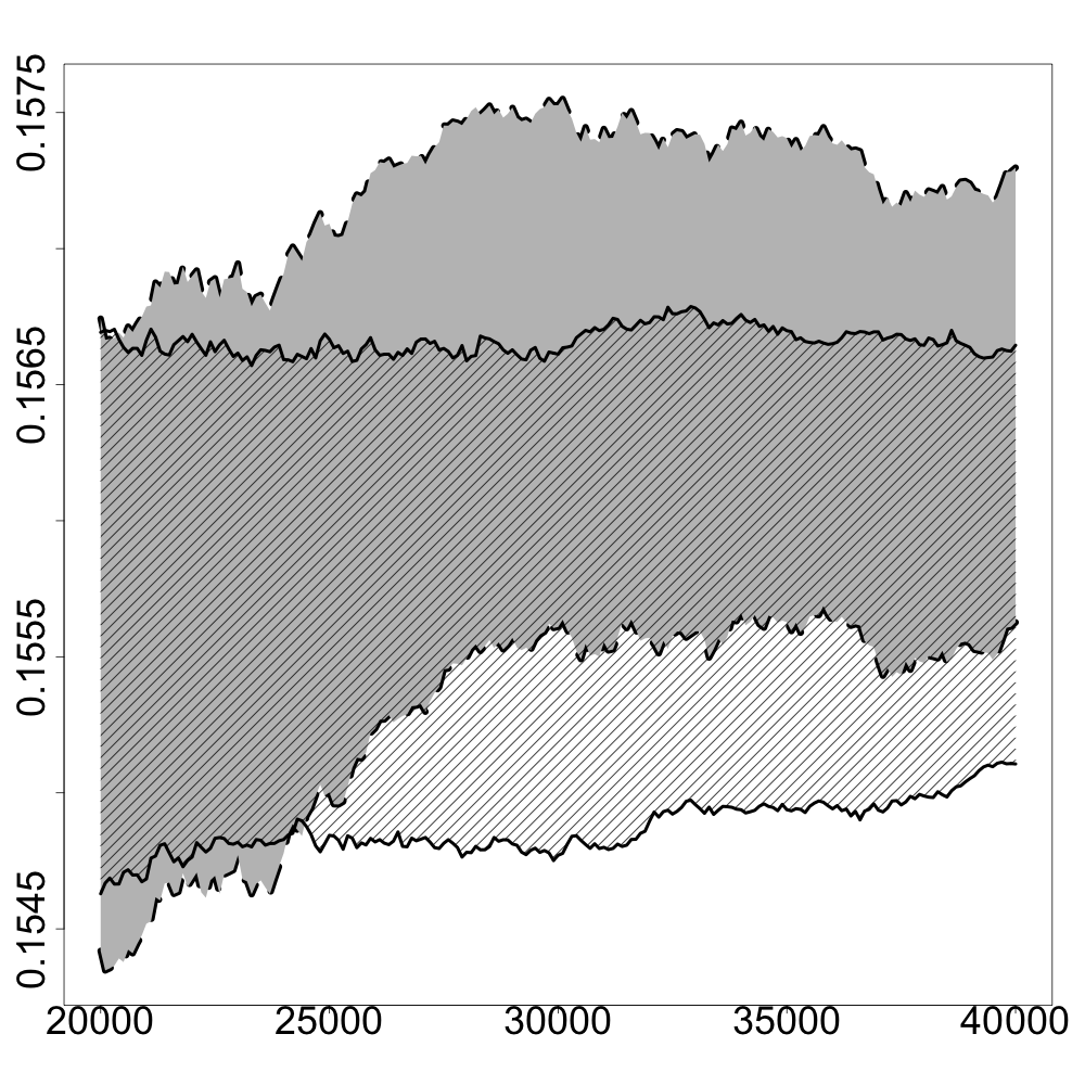 Figure 14
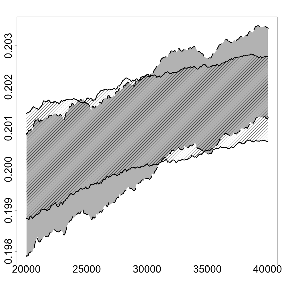 Figure 15
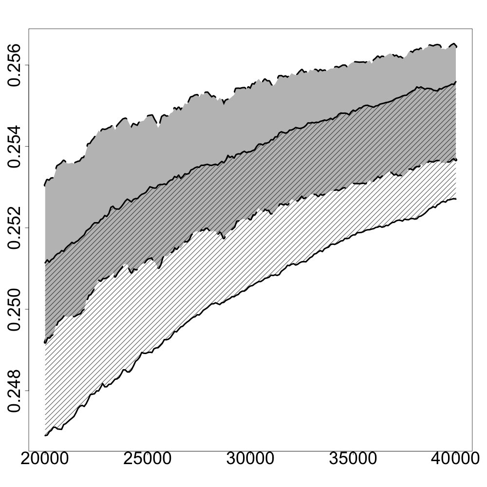 Figure 16
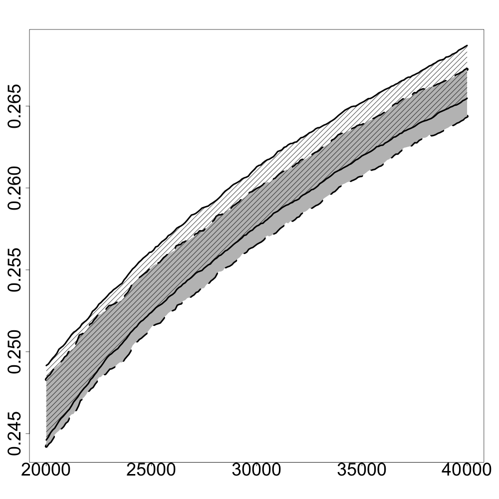 Figure 17
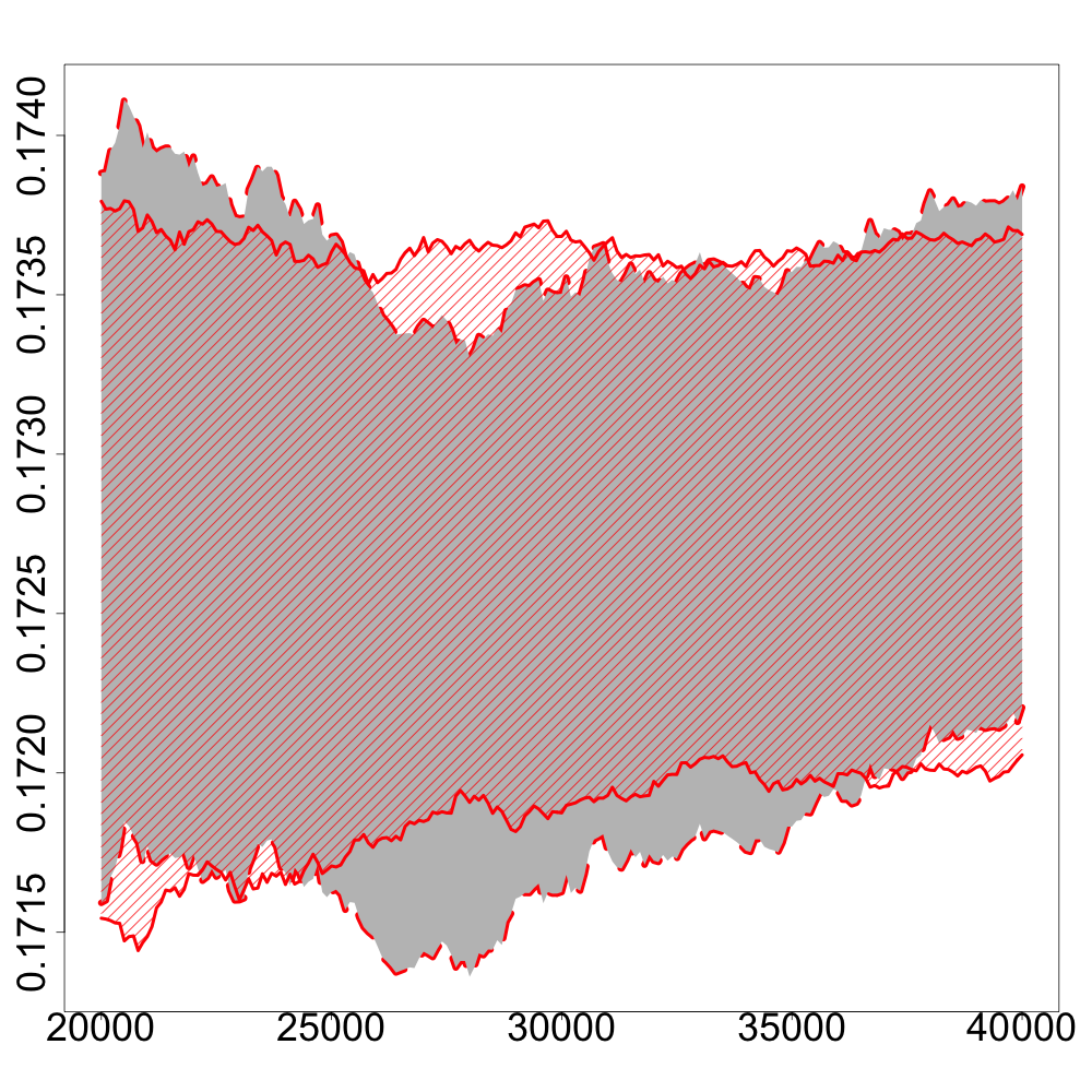 Figure 18
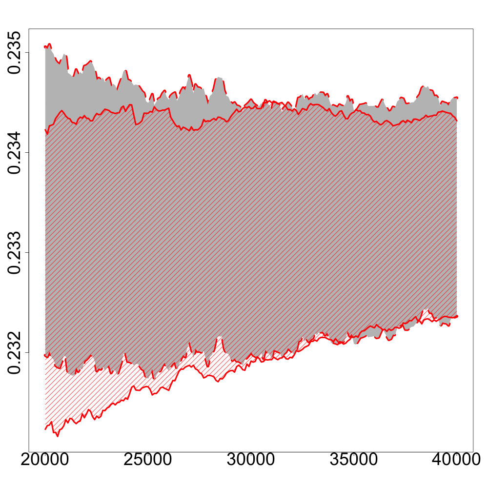 Figure 19
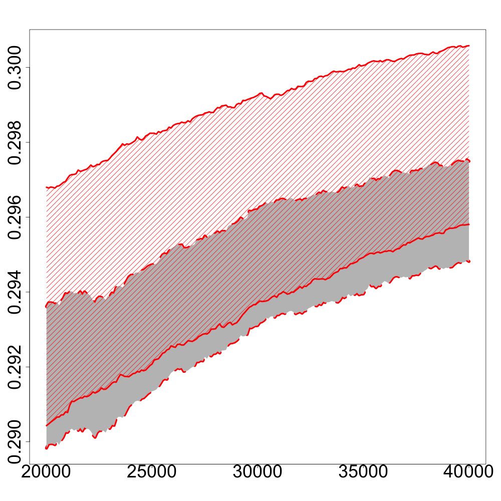 Figure 20
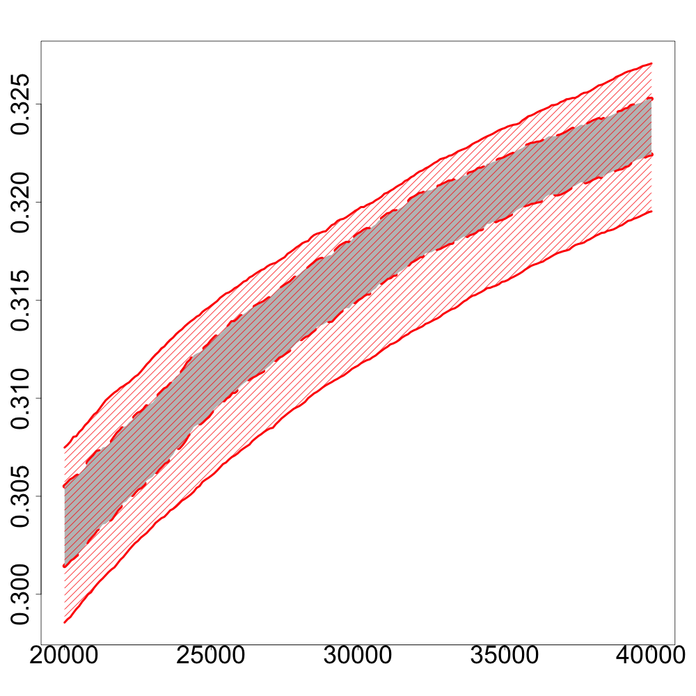 Figure 21
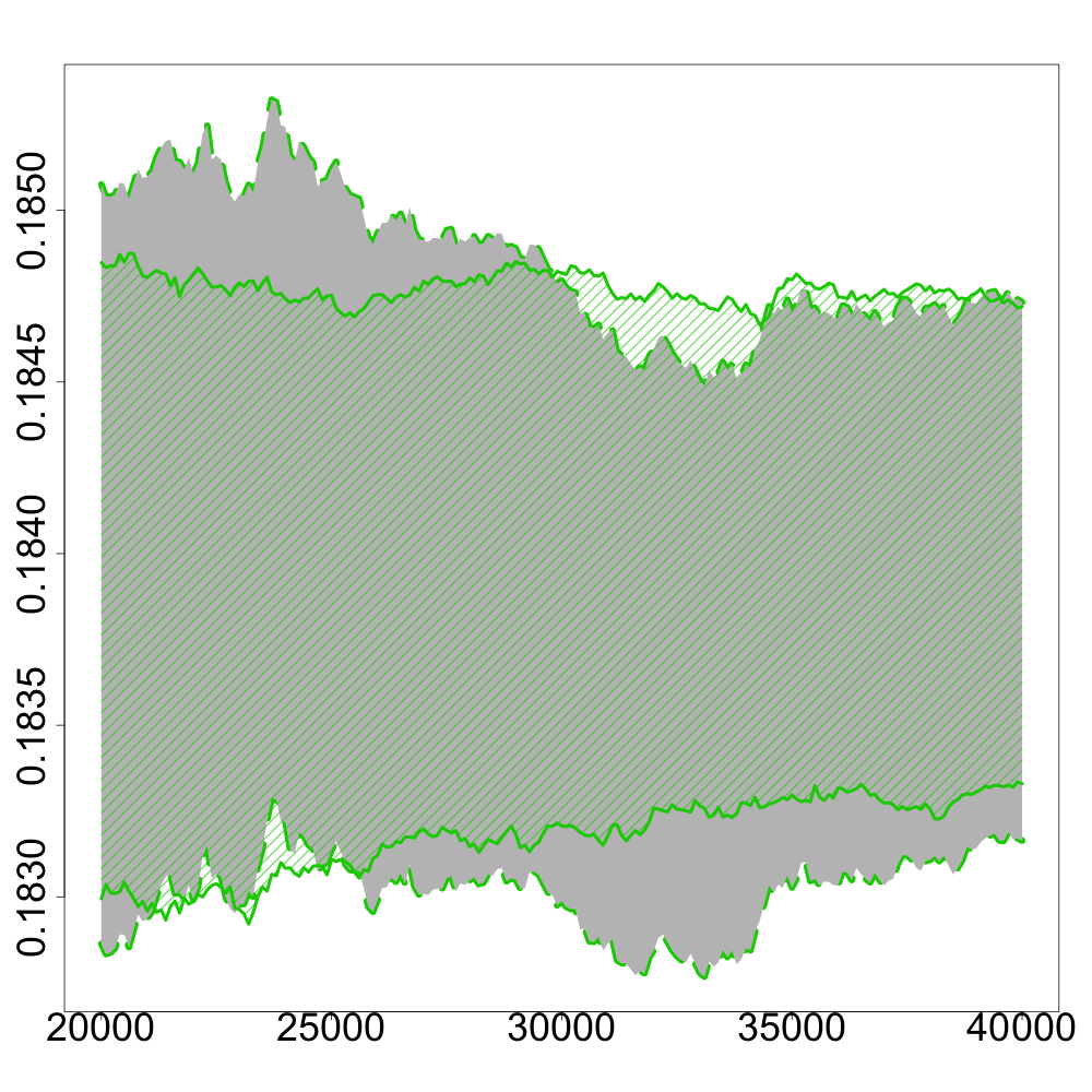 Figure 22
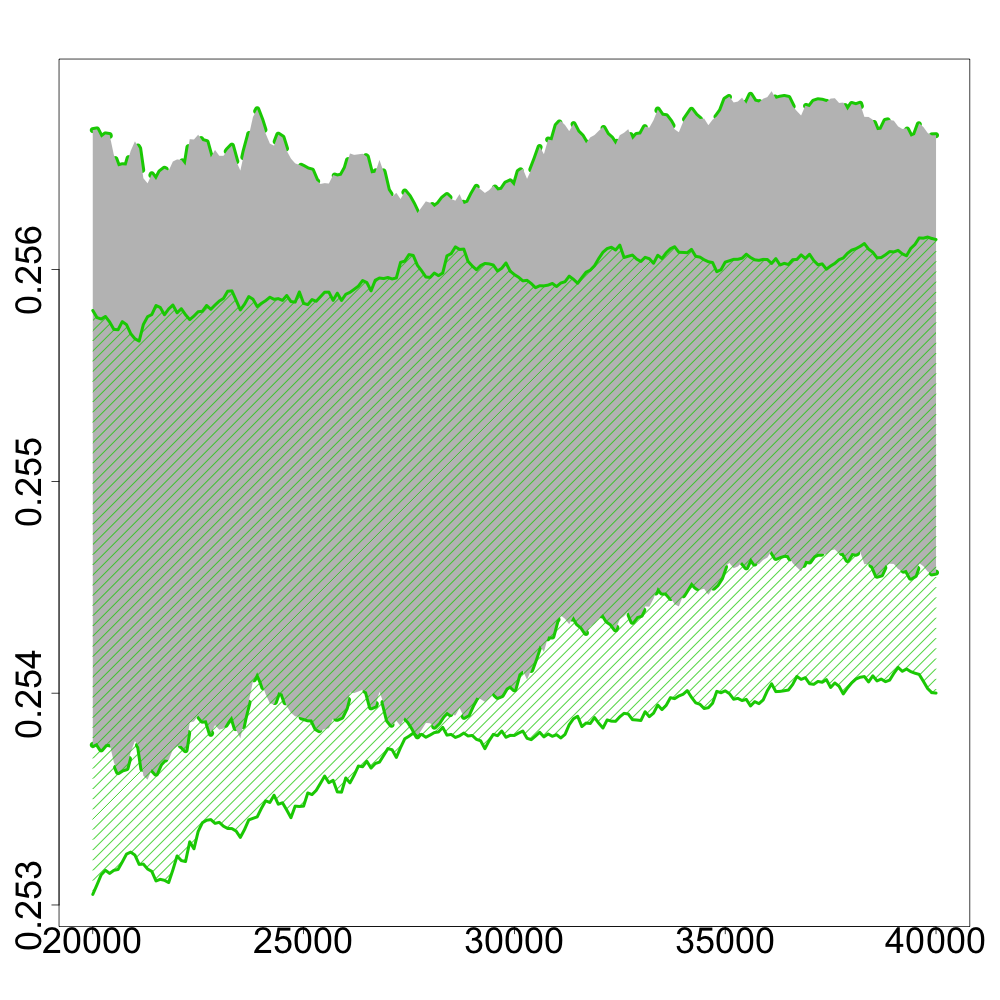 Figure 23
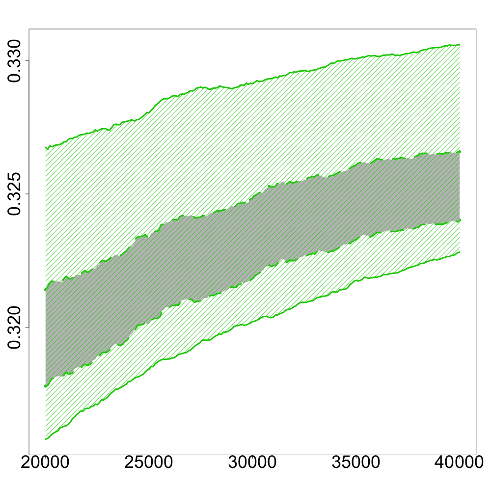 Figure 24
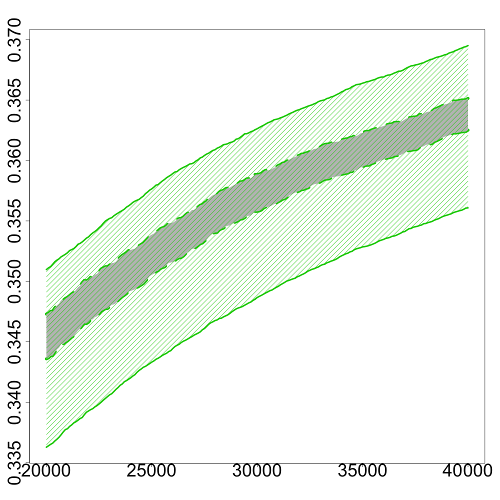 Figure 25
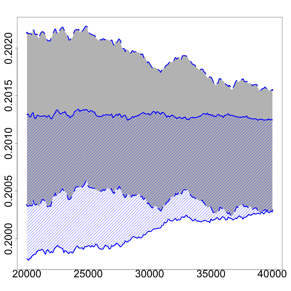 Figure 26
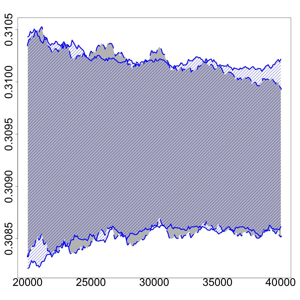 Figure 27
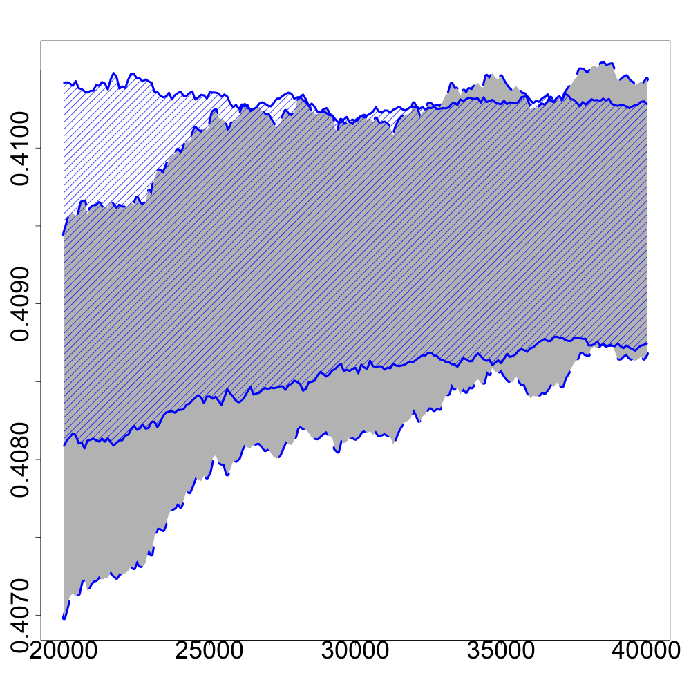 Figure 28
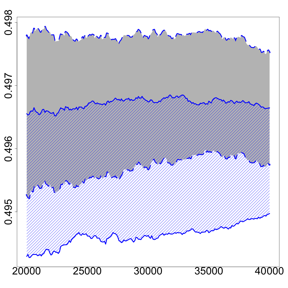 Figure 29
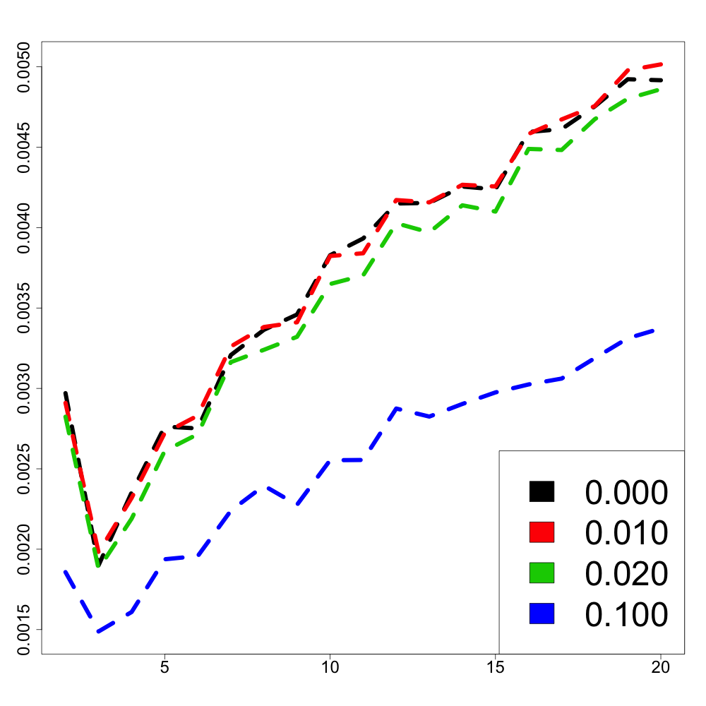 Figure 30
Peer Reviews
No public reviews on file for this paper yet. If you reviewed it on a platform where reviews are public (OpenReview, ICLR, NeurIPS, ICML), you can paste yours below so the community can read it here.
Videos
No videos yet. Explain this paper in a talk, walkthrough, or lecture? Add one.
Asymptotic distribution and convergence rates of stochastic algorithms for entropic optimal transportation between probability measures
Bernard Bercu and Jérémie Bigot
Université de Bordeaux
Institut de Mathématiques de Bordeaux et CNRS (UMR 5251)
Abstract.
This paper is devoted to the stochastic approximation of entropically regularized Wasserstein distances between two probability measures, also known as Sinkhorn divergences. The semi-dual formulation of such regularized optimal transportation problems can be rewritten as a non-strongly concave optimisation problem. It allows to implement a Robbins-Monro stochastic algorithm to estimate the Sinkhorn divergence using a sequence of data sampled from one of the two distributions. Our main contribution is to establish the almost sure convergence and the asymptotic normality of a new recursive estimator of the Sinkhorn divergence between two probability measures in the discrete and semi-discrete settings. We also study the rate of convergence of the expected excess risk of this estimator in the absence of strong concavity of the objective function. Numerical experiments on synthetic and real datasets are also provided to illustrate the usefulness of our approach for data analysis.
Jérémie Bigot is a member of Institut Universitaire de France (IUF), and this work has been carried out with financial support from the IUF.
Keywords: Stochastic optimisation; Convergence of random variables; Optimal transport; Entropic regularization; Sinkhorn divergence; Wasserstein distance.
AMS classifications: Primary 62G05; secondary 62G20.
1. Introduction
1.1. Optimal transport and regularized Wasserstein distances for data analysis
The statistical analysis of high-dimensional data using tools from the theory of optimal transport [48] and the notion of Wasserstein distance between probability measures has recently gained increasing popularity. When elements in a dataset may be represented as probability distributions, the use of the Wasserstein distance leads to relevant statistics in various fields such as fingerprints comparison [45], clinical trials [35], metagenomics [22], clustering of discrete distributions [50], learning of generative models [4], or geodesic principal component analysis [9, 44]. Wasserstein distances are also of interest in the setting of statistical inference from empirical measures for hypothesis testing on discrepancies between multivariate distributions [45].
However, the cost to evaluate a Wasserstein distance between two discrete probability distributions with supports of equal size is generally of order . Consequently, this evaluation represents a serious limitation for high-dimensional data analysis. To overcome this issue, Cuturi [15] has proposed to add an entropic regularization term to the linear program corresponding to a standard optimal transport problem. It leads to the notion of Sinkhorn divergence between two probability distributions which may be computed through an iterative algorithm where the cost of each iteration is of order . This proposal makes feasible the use of regularized optimal transportation distance for data analysis, and it has found various applications in generative models [27], multi-label learning [24], dictionary learning [43], or image processing [16, 29, 40], to name but a few. For an overview of regularized optimal transport applied to machine learning, we refer the reader to the recent book of Cuturi and Peyré [17] as well as to [2, 15] for deterministic algorithms on the computation of Sinkhorn divergences.
1.2. Main contributions and related works
This paper is inspired by the recent work of Genevay, Cuturi, Peyré and Bach [26] on a very efficient statistical procedure to evaluate the possibly regularized Wasserstein distance between an arbitrary probability measure and a discrete distribution with finite support of size . This statistical procedure is based on the well-known Robbins-Monro algorithm for stochastic optimisation [42] and its averaged version [38]. The keystone of their approach [26] is that can be rewritten in expectation form as
[TABLE]
where is a random vector drawn from the unknown distribution and is a suitable function of the regularization parameter . As it was shown in [26] on clouds of word embeddings, this statistical procedure is easy to implement with a low computational cost. For a sequence of independent and identically distributed random variables sharing the same distribution as , we shall extend the statistical analysis of [26] by proving that, for , the Robbins-Monro algorithm
[TABLE]
converges almost surely to a maximizer of . We also investigate the asymptotic normality of . It leads us to estimate the Sinkhorn divergence by the new recursive estimator
[TABLE]
Under standard assumptions in stochastic optimisation, we shall prove that
[TABLE]
as well as the asymptotic normality
[TABLE]
where the asymptotic variance \sigma^{2}_{\varepsilon}(\mu,\nu)={\mathbb{E}}\bigl{[}h_{\varepsilon}^{2}(X,v^{\ast})\bigr{]}-W_{\epsilon}^{2}(\mu,\nu) can also be estimated in a recursive manner. Finally, we analyze the rate of convergence of the expected excess risk . We shall prove that the expected excess risk goes to zero faster than in the absence of strong concavity of the objective function . These asymptotic results allow to better understand the convergence of stochastic algorithms for regularized optimal transport problems and to analyse the influence of their asymptotic variance on the quality of estimation. We shall also establish further results in the unregularized case where the regularization parameter .
The asymptotic behavior of empirical Wasserstein distances when both and are absolutely continuous measures has been extensively studied over the last years [18, 19, 20, 23, 41]. For probability measures supported on finite spaces, limiting distributions for empirical Wasserstein distance have been obtained in [45], while the asymptotic distribution of empirical Sinkhorn divergence has been recently considered in [8, 32].
1.3. Organisation of the paper
Notation and formulation of the possibly regularized optimal transportation problem are presented in Section 2. Asymptotic properties of our stochastic algorithms for the regularized optimal transport are stated in Section 3 and further results for the unregularized optimal transport are provided in Section 4. Numerical experiments illustrating our theoretical results on simulated and real data are given in Section 5, where we consider the problem of estimating an optimal mapping between the distribution of spatial locations of reported incidents of crime in Chicago and the locations of Police stations. All the proofs are postponed to Appendices Appendix A Three keystone lemmas. and Appendix B Proofs of the main results..
2. Formulation of the optimal transportation problem
Let and be two metric spaces. Denote by and the sets of probability measures on and , and by and the spaces of bounded and continuous functions on and , respectively. When and are finite sets, we identify the spaces and by the Euclidean spaces and . For and , let be the set of probability measures on with marginals and . As formulated in Section 2 of [26], the problem of entropic optimal transportation between and is as follows.
Definition 2.1**.**
For any , the Kantorovich formulation of the possibly regularized optimal transport between and is the following convex minimization problem
[TABLE]
[TABLE]
where is a lower semi-continuous function referred to as the cost function of moving mass from location to , is a regularization parameter, and KL stands for the Kullback-Leibler divergence, between and a positive measure on , up to the additive term , namely
[TABLE]
For , the quantity is the standard optimal transportation cost, while for , we shall refer to as the Sinkhorn divergence between the two probability measures and . The choice of the cost function depends on the application, and it usually reflects some prior knowledge on the data or the problem at hand. Throughout the paper, following [49, Part I-4], we consider cost functions satisfying the following assumption which holds for many standard choices. The cost is a lower semi-continuous function satisfying, for all ,
[TABLE]
where and are real-valued functions such that and . Under condition (2.3), is finite whatever is the value of the regularization parameter . Moreover, we always have , while can be negative for which comes from the expression of the KL divergence up to a constant additive term in Definition 2.1. We shall now define the dual and semi-dual formulations of the minimization problem (2.1) as introduced in [26]. For , these formulations are classical results in optimal transport known as Kantorovich’s duality. If the regularization parameter , it follows from [26, Proposition 2.1] that the dual expression of the minimization problem (2.1) is given by
[TABLE]
where
[TABLE]
The proof in [26] to derive the strong duality statement (2.4) relies on a formal application of Fenchel-Rockafellar’s theorem. Nevertheless, it appears that another proof can be found in the previous work [11] concerned by obtaining variational characterizations for the existence of a probability measure with given marginals, which is a problem closely related to regularized optimal transport, see also [33] for the connection between the Monge-Kantorovich and the Schrödinger problem. Indeed, it is known [17, Proposition 4.2] that the primal problem (2.1) can be refactored as the I-projection [13] problem
[TABLE]
with
[TABLE]
Hence, under condition (2.3), the duality result (2.4) can be derived from [11, Theorem 3.9]. The dual formulation (2.4) also follows as a particular instance of [12, Theorem 3.2] which considers unbalanced transport for marginals with different mass, but it is expressed as a maximization problem over the set of bounded functions rather than .
Then, arguing as in [26], the semi-dual of the convex minimization problem (2.1) is as follows. For any , the optimal transportation between and is obtained by solving the concave maximization problem
[TABLE]
where
[TABLE]
and for a given cost function satisfying (2.3), we define the -transform of as
[TABLE]
Thanks to condition (2.3), the sup in (2.6) is a max meaning that it exists a dual variable such that , see e.g. [49, Theorem 5.9]. In the regularized case , the existence of maximizers of (2.6) appears to be a more delicate issue. From (2.3), the cost belongs to the set of integrable functions with respect to . Hence, combining [13, Corollary 3.2] with the characterization (2.5) of regularized optimal transport, there exist a pair of functions belonging to and maximizing (2.4). However, an integrable function being not necessarily a bounded and continuous function, this result cannot be used to prove that is a pair of dual variables for the dual problem (2.4) when formulated as an optimisation over . The main difficulty seems to arise for unbounded costs. As a matter of fact, when the regularization parameter , the existence of a function maximizing (2.6) is proved in [25, Theorem 7] under the additional assumption that the cost function is bounded.
In the rest of the paper, we shall now suppose that the cost is not necessarily bounded, but that, for any , there exists such that . This identity is the keystone result which allows us to formulate the problem of estimating in the setting of stochastic optimization. Indeed, the semi-dual problem (2.6) can be rewritten in expectation form as
[TABLE]
where is a random vector drawn from the unknown distribution , and for and , In all the sequel, we will further assume that is a discrete probability measure with finite support in the sense that
[TABLE]
where the locations are a known sequence and stands for the standard Dirac measure. The weights are a known positive sequence that sum up to one. By a slight abuse of notation, we identify to the vector of with positive entries . We also denote by and the column vectors of with all coordinates equal to zero and one respectively, and by the standard inner product in . Following the terminology from [26], the discrete setting corresponds to the supplementary assumption that is also a discrete probability measure with finite support while the semi-discrete setting is the general case where is an arbitrary probability measure that is absolutely continuous with respect to the Lesbesgue measure and is a discrete measure with finite support (see e.g. Chapter 5 in [17] for an introduction to semi-discrete optimal transport problems and related references). When the size of the support of the measure is relatively small compared to the size of the support of , we would recommend to use the stochastic approach proposed in this paper. This suggestion is supported by the numerical results reported in Section 5. Now, if is the discrete measure (2.8), the semi-dual problem (2.6) can be reformulated as
[TABLE]
[TABLE]
where
[TABLE]
3. Asymptotic properties of stochastic algorithms for regularized optimal transport
Throughout this section, we assume that .
3.1. The stochastic Robbins-Monro algorithms
Our goal is to estimate the Sinkhorn divergence using a stochastic Robbins-Monro algorithm [42]. For any , the function , given by (2.10), is the mean value of where is a random vector drawn from the unknown distribution . For , the function , defined by (2.11), is twice differentiable in the second variable. The gradient vector as well as the Hessian matrix of can be easily calculated. More precisely, we have for any ,
[TABLE]
[TABLE]
where the component of the vector is such that
[TABLE]
Consequently, it follows from (2.10), (3.1) and (3.2) that the gradient vector and the Hessian matrix of are given by
[TABLE]
[TABLE]
One can observe that for any , is a negative semi-definite matrix. Therefore, if is a maximizer of (2.9), we have and for all , . It leads us to estimate the vector by the Robbins-Monro algorithm [42] given, for all , by
[TABLE]
where the initial value is a square integrable random vector which can be arbitrarily chosen and is a positive sequence of real numbers decreasing towards zero satisfying
[TABLE]
Two main issues arise with this Robbins-Monro algorithm. First of all, we clearly have from (3.5) that for any , which implies that zero is an eigenvalue of the Hessian matrix associated with the eigenvector Next, it follows from [15] that the maximizer of (2.9) is unique up to a scalar translation of the form for any . Throughout the paper, we shall denote by the maximizer of (2.9) satisfying which means that belongs to where is the one-dimensional subspace of spanned by . Therefore, to obtain a consistent estimator of it is necessary to slightly modify the Robbins-Monro algorithm (3.6).
Algorithm 1
A first strategy is as follows. It is easy to see from the expression (3.1) that the gradient is a vector of belonging to the linear space for any vectors and . Hence, if the initial value belongs to , one has immediately that is a stochastic sequence with values in the subspace . The analysis of its convergence to can thus be done by considering the restriction of the function to the linear subspace .
Algorithm 2
A second strategy is to estimate by the modified stochastic Robbins-Monro algorithm given, for all , by
[TABLE]
where is a square integrable random vector which can be arbitrarily chosen, the sequence satisfies (3.7), and where is a typically small positive parameter. The role played by is to overcome the fact that the Hessian matrix is singular. One can observe that if then for all , and thus Algorithm 2 is equivalent to Algorithm 1. By a slight abuse of notation, we shall also refer to Algorithm 1 as the case where and we refer to Algorithm 2 as the case where , although it is clear that depends on for Algorithm 2 when . One may also remark that Algorithm 2 corresponds to a stochastic ascent algorithm to compute a maximizer over of the strictly concave function
[TABLE]
where h_{\varepsilon,\alpha}(x,v)=h_{\varepsilon}(x,v)-\frac{\alpha}{2}\bigl{(}\langle v,\boldsymbol{v}_{J}\rangle\bigr{)}^{2}. An important role in the choice of will be the control of the smallest eigenvalue of the Hessian matrix . In the case , the objective function has a bounded gradient. As a matter of fact, since and , it follows that for all and ,
[TABLE]
which ensures that . In the case , we also have
[TABLE]
which implies that . The gradient of the objective function is clearly not bounded.
3.2. Almost sure convergence and asymptotic normality
Our first result concerns the almost sure convergence of the Robbins-Monro algorithms.
Theorem 3.1**.**
For both algorithms, we have the almost sure convergence
[TABLE]
We now focus our attention on the asymptotic normality of the Robbins-Monro algorithms. For any , let be the positive semidefinite matrix given by
[TABLE]
One can observe that for , \Gamma_{\varepsilon}(v^{\ast})={\mathbb{E}}\bigl{[}\pi(X,v^{\ast})\pi(X,v^{\ast})^{T}\bigr{]}-\nu\nu^{T}, since implies that . For any , denote
[TABLE]
We shall see in Lemma A.1 that for any , the matrix is negative semi-definite with . It means that the second smallest eigenvalue of the matrix is always positive. By a slight abuse of notation, we shall denote by the second smallest eigenvalue of the matrix . Moreover, let
[TABLE]
It follows from Remark A.1 that for any , the matrix is a negative definite. We shall also denote where stands for the maximum eigenvalue of the matrix . It is not hard to see that . Hereafter, in order to unify the notation, we put
[TABLE]
Theorem 3.2**.**
Assume that the step where
[TABLE]
Then, for both algorithms, we have the asymptotic normality
[TABLE]
where the asymptotic covariance matrix is the unique solutiuon of Lyapounov’s equation with
[TABLE]
Remark 3.1**.**
Theorem 3.2 is also true if with and , see Pelletier [37], Theorem 1. To be more precise, we have the asymptotic normality
[TABLE]
The convergence rate is clearly always slower than , which means that the choice outperforms the choice in term of convergence rate. However, in the special case , the restriction (3.16) involving the knownledge of is no longer needed.
Some refinements on the asymptotic behavior of the Robbins-Monro algorithms are as follows.
Theorem 3.3**.**
Assume that the step where satisfies (3.16). Then, for both algorithms, we have the quadratic strong law
[TABLE]
where is given by (3.18). Moreover, for any eigenvectors of the Hessian matrix , we have the law of iterated logarithm
[TABLE]
In particular,
[TABLE]
where is the matrix whose columns are the eigenvectors of .
Remark 3.2**.**
Theorem 3.3 also holds in the special case where with and , see Pelletier [36] Theorems 1 and 3. For example, the quadratic strong law (3.19) has to be replaced by
[TABLE]
In the special case , Theorem 3.3 is true without condition (3.16).
The explicit calculation of the asymptotic covariance matrix in (3.17) is far from being simple since there is no closed-form solution of equation (3.18). To overcome this issue, one may use the averaged Robbins-Monro algorithm given by which satisfies the second-order reccurence equation
[TABLE]
where the random vector is given by
[TABLE]
Our next result is devoted to the asymptotic behavior of the averaged Robbins-Monro algorithms.
Theorem 3.4**.**
For both algorithms, we have the almost sure convergence
[TABLE]
Moreover, assume that the step where and . Then, we have the asymptotic normality
[TABLE]
In particular, if the sequence is associated with Algorithm 1, convergence (3.25) can be rewritten as
[TABLE]
*where stands for the Moore-Penrose inverse of . *
Remark 3.3**.**
We already saw that the Hessian matrix is negative semi-definite with , which implies that its Moore-Penrose inverse is given by where are the negative eigenvalues of and are the associated orthonormal eigenvectors. Moreover,
[TABLE]
3.3. Estimation of the Sinkhorn divergence
Herafter, we focus our attention on the estimation of the Sinkhorn divergence . For that purpose, a natural recursive estimator of is given by
[TABLE]
Our first main result concerns the asymptotic behavior of the Sinkhorn divergence estimator .
Theorem 3.5**.**
Assume that the cost function satisfies for any ,
[TABLE]
Then, for both algorithms, we have the almost sure convergence
[TABLE]
Moreover, assume that the step where satisfies (3.16), or that where and . Then, for both algorithms, we have the asymptotic normality
[TABLE]
*where the asymptotic variance \sigma^{2}_{\varepsilon}(\mu,\nu)={\mathbb{E}}\bigl{[}h_{\varepsilon}^{2}(X,v^{\ast})\bigr{]}-W_{\epsilon}^{2}(\mu,\nu). *
Remark 3.4**.**
The asymptotic variance can be estimated by
[TABLE]
Via the same lines as in the proof of (3.30), we can show that a.s. Therefore, using Slutsky’s Theorem, it follows from (3.31) that
[TABLE]
Convergence (3.33) allows us to construct confidence intervals for the Sinkhorn divergence as illustrated in the numerical experiments of Section 5.
Our second main result is devoted to the expected excess risk of the Sinkhorn divergence estimator . It follows from (3.28) that
[TABLE]
Hence, the expected excess risk of is defined as the non-negative quantity
[TABLE]
It is well known that only assuming concavity of the objective function leads to convergence rates for the expected excess risk of the order for the Robbins-Monro algorithm. This rate of convergence cannot be improved without supplementary assumptions such as the strong concavity of the objective function , which leads to faster rates of convergence of the order for some which depends on the decay of the step where . We refer the reader to [6], [7], [28] for a recent overview on the convergence rates of first-order stochastic algorithms.
However, as it was already shown in [26], the objective function in the semi-dual problem (2.6) cannot be strongly concave, even by restricting the maximization to the subset . Indeed, the gradient being bounded on , it follows that is a Lipschitz function, and thus it cannot be strongly concave on , see e.g. Section 3.2 in [7]. Nevertheless, for the stochastic optimization problem (2.6), it is possible to derive rates of convergence faster than for the expected excess risk . To this end, we borrow some ideas related to the so-called notion of generalized self-concordance coming from the recent contribution of Bach [6] and leading to faster rates of convergence for stochastic algorithms with non-strongly concave objective functions.
Theorem 3.6**.**
Assume that is a random vector such that, for any integer , is finite. Moreover, assume that the step where and . In addition, suppose that and
[TABLE]
Then, there exists a positive constant such that for any ,
[TABLE]
Remark 3.5**.**
It is easy to see that the assumption implies that . Consequently, the condition (3.35) is not really restrictive and it is fulfilled by a suitable choice of depending on . By inequality (A.4) and Remark A.2, one has the following bounds which are used to choose the parameter in the numerical experiments carried out in Section 5. Finally, it follows from (3.34) together with inequality (3.36) that
[TABLE]
Consequently, if , inequality (3.37) shows that the expected excess risk of may converge to zero faster than when the sequence is given by Algorithm 1.
4. Further results on the unregularized case
We now focus our attention on the unregularized case where . The function , defined by (2.11), is not differentiable. Nevertheless, as remarked in [26], it follows from (2.11) that for any , a supergradient of at is
[TABLE]
where denotes the vector of with all entries equal to zero expect the -th which is equal to one, that is , where
[TABLE]
One can note that for and , the integer may be not unique. In this case, the set of supergradients is not a singleton. In contrast with the regularized case where , the function does not necessarily have a unique maximizer over . To estimate such a maximizer , which is assumed to belong to , we shall consider a standard stochastic supergradient ascent given, for all , by
[TABLE]
where the sequence satisfies (3.7), is a typically small positive parameter and is any supergradient of at of the form (4.1). Therefore, a recursive estimator of is given by
[TABLE]
In order to investigate the asymptotic properties of the random sequences and , two issues need to be addressed: the regularity of the function and the uniqueness of its maximizer over . In the discrete setting, the function is clearly not differentiable. However, in the semi-discrete setting where is absolutely continuous, the differentiability of has been proved in [31] under appropriate regularity assumptions on the cost function and the measure . More precisely, by [31, Theorem 2.1], we obtain the following conditions ensuring the -smoothness of .
Proposition 4.1**.**
Assume that that . Moreover, suppose that
**(i): **
For all , the function is continuous.
**(ii): **
The measure is absolutely continuous with bounded and compactly supported probability density function.
**(iii): **
For any and for all , the set has zero Lebesgue measure.
Then, the function is continuously differentiable on ,
[TABLE]
where is any supergradient of at of the form (4.1).
Guaranteeing the uniqueness of the maximizer of over is more involved. In particular, in the semi-discrete setting, we are not aware of any sufficient conditions ensuring such a property. Nevertheless, if one assumes the uniqueness of up to scalar translations, then under the assumptions of Proposition 4.1, it follows that is continuous. Therefore, arguing as in the proofs of Theorem 3.1 and Theorem 3.5, one obtains under the assumptions of Proposition 4.1 that
[TABLE]
and
[TABLE]
Furthermore, under additional assumptions it follows from [34, Theorem 6] that is twice continuously differentiable. Nevertheless, in contrast to the regularized case, the second smallest eigenvalue of may be zero. Therefore, the proof of the asymptotic normality for and is much more tricky and left open for future work.
5. Statistical applications and numerical experiments
In this section, we report results on numerical experiments for probability measures and with supports included in for using synthetic and real data sets. All numerical experiments are carried out with the statistical computing environment R [39], and they are based on iid samples from . We mainly investigate the numerical behavior of the two recursive estimators and . The reader has to keep in mind that the estimators and depend on the positive value of the regularization parameter as well as on the positive value of and the statistical characteristics of and . However, for the sake of simplicity, we have chosen to denote them as and . We carry out our numerical experiments for different values of to illustrate the convergence of the recursive algorithms proposed in this paper as increases. Following the discussion in Section 3 on the calibration of the step size for , we took with and where stands for . In the unregularized case of Section 4, we took where is the smallest value of regularization used in these numerical experiments. The cost function is chosen as the standard Euclidean distance,
[TABLE]
In our numerical experiments, we have found that Algorithm 1 with and , and Algorithm 2 with and share the same numerical behavior for all sufficiently large values of , that is . Consequently, we only report here the results obtained with Algorithm 1.
5.1. Discrete setting in dimension two
We first consider a setting in dimension with discrete probability measures, and we investigate the regularized case where . The measure is assumed to be the uniform measure on a grid made of regularly spaced points. The measure is obtained by projecting a mixture of Gaussian densities on an regular grid of . The cardinality of its support varies in the numerical experiments. The two measures are displayed in Figure 1 for different values of .
The computation of the Sinkhorn divergence is done via the package Barycenter111https://cran.r-project.org/package=Barycenter. It allows us to solve the semi-dual maximization problem (2.6) using the Sinkhorn algorithm [15] which is a fixed point iteration algorithm for obtaining a solution of the primal problem (2.1) of the form
[TABLE]
where \mbox{\boldsymbol{C}}\in{\mathbb{R}}^{I\times J} is the cost matrix, is a pair of optimal dual variables and denotes the entrywise exponential. To obtain such a pair of dual variables in an iterative way, the Sinkhorn algorithm alternately scales the row and column sums of matrices written in the form (5.1) to match the marginals and , that is and , where denotes the elementwise ratio between vectors. Hence, at each iteration, the computational cost of the Sinkhorn algorithm is of the order . An advantage of stochastic algorithms for optimal transport is that the computational cost of the recursive estimators and at each iteration of (3.6) and (3.32) is only of order as discussed in details in [26]. Moreover, the computation of these estimators do not require the full knowledge of the measure , and the storage of the full cost matrix . The computational cost at each iteration of the Sinkhorn algorithm can be reduced by using a greedy coordinate descent algorithm referred to as the Greenkhorn algorithm [3] which consists in only updating one row or column of a matrix written in the form (5.1) by selecting the one that most violates the constraint that its row and columns sums should match the desired marginal and . As described in [3], it is possible to implement this algorithm in such a way that the computational cost at each iteration is linear in the dimension of the input measures that is of order . A stochastic version of the Greenkhorn algorithm has also been proposed in [1], where, instead of selecting the column or row which most violates the constraint, one row or column is randomly selected according to probability chosen in such a way that the columns and rows with highest violation are updated more frequently. Note that the stochastic Greenkhorn algorithm makes use of the full knowledge of , and it is thus a stochastic algorithm of a different nature than the Robbins-Monro algorithm investigated in this paper. In particular, our approach does not use the knowledge of , and the recursive estimators estimators and have not been considered so far in the literature. In the discrete setting, it is proposed in [26] to use a stochastic averaged gradient algorithm (which uses the knowledge of ) to estimate , and we refer to [26, Section 3] for detailed experiments on the comparison of this approach to the Sinkhorn algorithm.
In Figure 2, we report numerical results on the comparison between the recursive estimator and the numerical approximation of using either the Greenkhorn algorithm or its stochastic version as a function of the iterations whose computational costs are linear in the dimension of the input measures. The output of the Sinkhorn algorithm is used as the ground truth for . Using the results from Section 3, one can construct confidence intervals for the Sinkhorn divergence between and by considering
[TABLE]
to be approximately normally distributed. One can see in Figure 2 that the confidence intervals always contain the value for and all values of and cardinality of the support of . The Greenkhorn algorithm and its stochastic version perform similarly. For small values of and large values of , we observe that these algorithms converge in very few iterations. However, for larger values of , that is larger sizes of the support of , and for small values of , the recursive estimator clearly outperforms such Greenkhorn algorithms in the number of required iterations to obtain a satisfactory approximation of .
5.2. Semi-discrete setting in dimension
Simulated data. We now consider a synthetic example where is an absolutely continuous measure obtained as a mixture of three Gaussian densities with support truncated to for . We shall let the dimension growing as well as the size of the support of when increases. For each , is chosen as the uniform discrete probability measure supported on points drawn uniformly on the hypercube . We report results for . There exist various algorithms for semi-discrete optimal transport in the unregularized case to evaluate . We refer to [34, Section 1.2] for an overview and a discussion of their computational cost. These approaches are based on the knowledge of the measure that is generally projected over a partition of . However, available implementations222https://github.com/mrgt/PyMongeAmpere and https://cran.r-project.org/package=transport based on the works in [30, 31] are typically restricted to the dimension . For larger values of , projecting on a sufficiently finite partition becomes computationally prohibitive, and storing the resulting cost matrix becomes too memory demanding which makes a direct use of Sinkhorn or Greenkhorn algorithms not feasible. Moreover, to the best of our knowledge, apart from stochastic approaches as in [26], there is no other method to evaluate in the semi-discrete setting.
In the following numerical experiments, we briefly study how the recursive estimators and scales with increasing dimension and support size , for , in both unregularized and regularized cases. First, we observe that for various values of the regularization parameter and the dimension , the confidence intervals obtained via the Gaussian approximation (5.2) give an accurate estimation of the range of variation of calculated by Monte Carlo simulations as shown in Figure 3. Note that, in these numerical experiments, we conjecture that the Gaussian approximation (5.2) also holds for .
Finally, in Figure 4, we display the evolution of the size of the confidence intervals for (after iterations) based on the Gaussian approximation (5.2) as the dimension increases and for . The size of these confidence intervals is clearly an increasing function of . This suggests that the number of iterations should increase with to keep the same level of accuracy when estimating .
Real data. We consider a dataset containing spatial locations of reported incidents of crime with the exception of murders in Chicago in 2014, publicly available at https://data.cityofchicago.org. These data points are ordered in a chronological manner from January to December. Victims’ addresses are shown at the block level only. Specific locations are not identified in order to protect the privacy of victims and to have a sufficient amount of data for the statistical analysis. For simplicity, spatial locations of the city of Chicago are represented on the unit square . For the year 2014, spatial locations of reported incidents of crime in Chicago are available. They are displayed in Figure 5(a). Chicago has Police stations whose locations are shown in Figure 5(b) with a kernel density estimation of the unknown distribution of crime locations.
We assume that Police stations have the same capacity, and they are thus modeled by the uniform discrete measure on these locations. We first report the evolution of the recursive confidence intervals for various values of in the unregularized and regularized cases. To evaluate the convergence of our stochastic algorithm, we have also computed the values of where is the standard empirical measure approximating .
For the regularized case , we used the Sinkhorn algorithm. For , we followed the method proposed in [30] that is specific to the Euclidean cost and implemented in the package Transport. One can observe in Figure 5(c) a very good convergence of the algorithm for different values of .
Finally, we consider the problem of estimating an optimal partition of the city of Chicago into 23 districts matching expected locations of crimes with the capacity of Police stations so that the expected cost of travelling from a station to a crime’s location is minimal. This can be done by estimating, in the unregularized case, an optimal map which pushes forward onto . Since is absolutely continuous, it is well-known [10, 14] that there exists a unique optimal mapping which pushes forward onto . This mapping is clearly piecewise constant. It follows from Corollary 1.2 in [31] that for all ,
[TABLE]
where is any maximiser of the semi-dual problem (2.6). The sets are the so-called Laguerre cells that correspond to an important concept from computational geometry (see e.g. [30, 31] and Chapter 5 in [17]). Then, based on a sample from , it is natural to estimate the Laguerre cells by
[TABLE]
where stands for -entry of the vector obtained from (4.2). An example of estimated Laguerre cells is given in Figure 5(d). We observe that cells of small size are located near the modes of the estimated distribution of crime locations.
Appendix A
Three keystone lemmas.
The proofs of the main results of this paper rely on three keystone lemmas. The first one is devoted to the spectrum of the Hessian matrix given by (3.14). Denote by its real eigenvalues and by its associated orthonormal eigenvectors, where and . Let
[TABLE]
Lemma A.1**.**
For any , the Hessian matrix is negative semi-definite with . More precisely,
[TABLE]
where for all and for all , the positive eigenvalues are given by
[TABLE]
with
[TABLE]
Moreover, we also have
[TABLE]
which implies that
[TABLE]
Remark A.1**.**
For any , denote
[TABLE]
where stands for the maximum eigenvalue of the Hessian matrix given by (3.15). It is not hard to see that for all , the matrix is negative definite. More precisely, its negative eigenvalues are and
[TABLE]
As a matter of fact, , while for any , .
Proof.
First of all, we obtain from (3.5) together with (3.14) that for any ,
[TABLE]
where, for all ,
[TABLE]
We deduce from Theorem 1 in [47] that for any , , and that the positive eigenvalues of are given by (A.2) except the smallest one which is associated, for all , to the same eigenvector . Consequently, it follows from (A.5) that is a negative semi-definite matrix such that . In addition, (A.5) clearly leads to (A.1). Furthermore, equality (A.3) follows (3.14) and (3.4) which implies the fact that \nu={\mathbb{E}}\bigl{[}\pi(X,v^{\ast})\bigr{]}. Hereafter, we have the decomposition
[TABLE]
where, for all ,
[TABLE]
It follows from Theorem 6 and inequality (5.11) in [46] that the second smallest eigenvalue of is lower bounded by for all . Hence, we deduce inequality (A.4) from this lower bound and the decomposition (A.6), which completes the proof of Lemma A.1. ∎
The second lemma deals with the Taylor expansion of the concave function . It allows us to control the excess risk of our Sinkhorn divergence estimator. Let be the strictly increasing function defined, for all positive , by
[TABLE]
One can observe that we always have .
Lemma A.2**.**
For any , we have
[TABLE]
where
[TABLE]
and
[TABLE]
where for all and for all , the positive eigenvalues are given by (A.2). Moreover, for any ,
[TABLE]
Moreover, assume that for some positive constant . Then,
[TABLE]
Remark A.2**.**
On the one hand, we deduce from (A.2) that for all and for all , which means that . On the other hand, inequalities (A.7) and (A.10) are also true for the strictly concave function given by (3.9). As a matter of fact, it is only necessary to replace and by and in (A.7). Moreover, since , one can observe for (A.10) that for any ,
[TABLE]
Inequality (A.10) is typically a consequence of the so-called notion of generalized self-concordance as introduced in [5] for the study of logistic regression. Generalized self-concordance has been widely used in [6] to obtain rates of convergence of order for non-strongly convex functions using a constant step size.
Proof.
The first step of the proof is to establish a second-order Taylor expansion of the concave function . For any and for all in the interval , denote . Let be the function defined, for all , by
[TABLE]
The second-order Taylor expansion of with integral remainder is given by
[TABLE]
However, it follows from the chain rule of differentiation that for all ,
[TABLE]
Hence, as , and , we obtain from (A.12) that for any ,
[TABLE]
We already saw in (A.5) that -\varepsilon A_{\varepsilon}(v)={\mathbb{E}}\bigl{[}A_{\varepsilon}(X,v)\bigr{]}. In addition, for all ,
[TABLE]
which implies by (A.8) and (A.9) that . Consequently, we deduce from (A.13) that for any ,
[TABLE]
which clearly leads to
[TABLE]
In order to prove (A.10), we have to compute the third-order derivative of the function which is given by
[TABLE]
where for all ,
[TABLE]
A direct calculation of this third-order derivative is not easy. However, it follows from (3.4) that
[TABLE]
where for all , . Moreover, one can notice that for all and for all ,
[TABLE]
Consequently, we obtain from the chain rule of differentiation together with (A.14) and (A.15) that
[TABLE]
where for all ,
[TABLE]
In the same way, we also obtain from (A.15) and (A.16) that
[TABLE]
where for all ,
[TABLE]
Hence, we deduce from the previous calculation that for all ,
[TABLE]
and
[TABLE]
One may remark that for all , the variance term . More precisely, and are the mean and the variance of a discrete random variable with values in and distribution . Moreover, the third cumulant of the random variable is given, for all , by
[TABLE]
Therefore, we obtain from (A.19) and (A.20) that for all ,
[TABLE]
It is not hard to see from the Cauchy-Schwarz inequality that
[TABLE]
Consequently, inequality (A.21) ensures that for all ,
[TABLE]
which implies, via (A.16) and (A.17), that for all ,
[TABLE]
Inequality (A.22) means that the function satisfies the so-called generalized self-concordance property as defined in Appendix B of [6]. We are now in position to prove (A.10). Let be the function defined, for all , by
[TABLE]
The second-order Taylor expansion of with integral remainder is given by
[TABLE]
We already saw that for all ,
[TABLE]
Hence, as , and , we obtain from (A.23) that for any ,
[TABLE]
For any , we clearly have . Consequently, it follows from (A.22) that for all ,
[TABLE]
By taking into (A.25), we find from (A.25) that for all ,
[TABLE]
Integrating by parts, we deduce from (A.24) and (A.26) that for any ,
[TABLE]
Finally, as , , we obtain from (A.7) together with (A.27) that for any ,
[TABLE]
which is exactly what we wanted to prove. It only remains to prove inequality (A.11). We shall proceed as in the proof of Lemma 13 in [6]. It follows from (A.22) that for all ,
[TABLE]
By integrating (A.28) between [math] and , we obtain that for all ,
[TABLE]
which leads to
[TABLE]
However, we already saw that which implies that . By integrating (A.29) between [math] and , we find that for any ,
[TABLE]
since and . Let be the strictly increasing function defined, for all positive , by
[TABLE]
We immediately deduce from (A.30) that, as soon as for some positive constant ,
[TABLE]
proving that inequality (A.11) holds for . Hereafter, assume that where . If , we clearly obtain from (A.30) that
[TABLE]
meaning that inequality (A.11) is satisfied. Moreover, assume that . We infer from (A.29) that
[TABLE]
which implies that
[TABLE]
The assumption clearly implies that . Finally, we deduce from (A.31) that
[TABLE]
It ensures that (A.11) holds for any , completing the proof of Lemma A.2. ∎
The third lemma concerns a sharp upper bound for a very simple recursive inequality which will be useful in the control the excess risk of our Sinkhorn divergence estimator.
Lemma A.3**.**
Let be a sequence of positive real numbers satisfying, for all , the recursive inequality
[TABLE]
where and are positive constants satisfying , , and with in the special case where . Then, there exists a positive constant such that, for any ,
[TABLE]
Proof.
One can observe that the first term on the right hand side inequality (A.33) is always non-negative thanks to the condition . We shall proceed as in the proof of Theorem 1 in [7]. It follows from (A.33) that for all ,
[TABLE]
First of all, we focus our attention on the case where . We clearly have
[TABLE]
Hence, we obtain from the elementary inequality that
[TABLE]
where
[TABLE]
Deriving an upper bound for the second term in the right hand side of inequality (A.35) is more involved. To this end, we denote for all ,
[TABLE]
with the convention that . For some interger which will be fixed soon, we have the decomposition
[TABLE]
Therefore, noticing that for all , we obtain that
[TABLE]
However, one can observe that for all ,
[TABLE]
which implies that
[TABLE]
Furthermore, we clearly have
[TABLE]
In addition, by choosing the integer such that with , we obtain that where
[TABLE]
Hence, it follows from inequality (A.39) that
[TABLE]
Consequently, we deduce from (A.37) together with (A.38) and (A.40) that the second term in the right hand side of (A.35) is bounded by
[TABLE]
Therefore, we obtain from (A.35), (A.36) and (A.41) that for all ,
[TABLE]
It implies that there exists a positive constant such that for all ,
[TABLE]
Hereafter, we assume that . It is not hard to see that
[TABLE]
Consequently,
[TABLE]
Moreover, for all , we also have
[TABLE]
which implies that
[TABLE]
Hence,
[TABLE]
leading to
[TABLE]
since . Thus, we obtain from (A.35) together with (A.42) and (A.43) that
[TABLE]
Finally, as , we deduce from (A.44) that there exists a positive constant such that for all ,
[TABLE]
which achieves the proof of Lemma A.3. ∎
Appendix B
Proofs of the main results.
We shall now proceed to the proofs of the main results of the paper. We recall that is a sequence of independent and identically distributed random vectors sharing the same distribution as . We shall denote by the -algebra of the events occurring up to time , that is .
Proof of Theorem 3.1. We obtain from (3.8) and (3.23) that for all ,
[TABLE]
where the random vector satisfies Hence, it follows from (3.9) that
[TABLE]
where, for all , The gradient is a continuous function from to such that . Moreover, for any such that ,
[TABLE]
As a matter of fact, if belongs to and , then and , which ensures that (B.3) is satisfied on . Moreover, if belongs to , then since has a unique maximum on . It means that (B.3) also holds true on . Denote and . Obviously, for any , . In addition, it follows from the upper bound (3.11) that
[TABLE]
Hence, we deduce from (B.4) that for all , where . Therefore, all the assumptions of Theorem 1.4.26 of Duflo [21] are satisfied and we can conclude from (3.8) that a.s. which achieves the proof of Theorem 3.1.
Proof of Theorem 3.2. We shall now prove the asymptotic normality of the modified Robbins-Monro algorithm (3.8) which can be rewritten as
[TABLE]
where . First of all, we clearly have . Moreover, where, thanks to (3.1) and (3.23),
[TABLE]
with
It immediately follows from the above identity that
[TABLE]
However, we can deduce from Theorem 3.1 that
[TABLE]
Hence, it follows from (B.6), (B.7) together with Theorem 3.1 that
[TABLE]
where is given by (3.13). Moreover, we obtain from (3.11) and the upper bound (B.4) that
[TABLE]
which implies that
[TABLE]
Therefore, as converges almost surely to , we find from (B.8) that
[TABLE]
Furthermore, we already saw that . Consequently, and it follows from (A.10) that for all , \nabla H_{\varepsilon,\alpha}(v)=A_{\varepsilon,\alpha}(v^{\ast})(v-v^{\ast})+O\bigl{(}||v-v^{\ast}||^{2}\bigr{)}. Finally, under the assumption (3.16) on the maximum eigenvalue of , we obtain from Theorem 1 of Pelletier [37] or Theorem 2.3 in the more recent contribution of Zhang [51] that \sqrt{n}\bigl{(}\widehat{V}_{n}-v^{\ast}\bigr{)}\mathrel{\mathop{\kern 0.0pt\longrightarrow}\limits^{{\mbox{\calcal L}}}}\mathcal{N}_{J}\bigl{(}0,\gamma\Sigma^{\ast}\bigr{)}, which is exactly what we wanted to prove.
Proof of Theorem 3.3. We already saw from (B.5) that for all , \widehat{V}_{n+1}=\widehat{V}_{n}+\gamma_{n+1}\bigl{(}\nabla H_{\varepsilon,\alpha}(\widehat{V}_{n})+\varepsilon_{n+1}\bigr{)} where and
[TABLE]
In addition, we also have from (B.9) that a.s. Then, the quadratic strong law (3.19) immediately follows from Theorem 3 in [36]. We also deduce the law of iterated logarithm (3.20) from Theorem 1 in [36], which completes the proof of Theorem 3.3.
Proof of Theorem 3.4. The proof of the almost sure convergence (3.24) follows from (3.12) by the Cesàro mean convergence theorem [21], while the proof of the asymptotic normality (3.25) is a direct consequence of the averaging principle for stochastic algorithms given e.g. by Theorem 2 of Polyak and Judistsky [38]. In order to prove (3.26), one can observe that if is the sequence associated with Algorithm 1, then for all , belongs to . It follows from Lemma A.1 that the Moore-Penrose inverse of is given by (3.27). Hence, if one denotes by the orthogonal projection on , the asymptotic normality (3.26) is a direct consequence of the asymptotic normality (3.25) combined with the facts that P_{J}\bigl{(}\overline{V}_{n}-v^{\ast}\bigr{)}=\overline{V}_{n}-v^{\ast} and which implies that
Proof of Theorem 3.5. We now focus our attention on the Sinkhorn divergence estimator which can be separated into two terms,
[TABLE]
where, for all , . On the one hand, it follows from (2.9) and (2.10) that is a continuous function from to such that . Consequently, we immediately deduce from (3.12) and the Cesàro mean convergence theorem [21] that
[TABLE]
On the other hand, denote It is not hard to see that is a locally square integrable real martingale. Its predictable quadratic variation is given by
[TABLE]
We deduce once again from the Cesàro mean convergence theorem that
[TABLE]
where the asymptotic variance \sigma^{2}_{\varepsilon}(\mu,\nu)={\mathbb{E}}\bigl{[}h_{\varepsilon}^{2}(X,v^{\ast})\bigr{]}-W_{\epsilon}^{2}(\mu,\nu). Note that using the convexity the function and the positivity of the cost , it can be easily shown that, for all and ,
[TABLE]
and thus the integrability condition (3.29) combined with the upper bound (B.13) ensures that is finite. Hence, we obtain from (B.12) together with the strong law of large numbers for martingales given, e.g. by Theorem 1.3.24 of Duflo [21] that
[TABLE]
Therefore, the almost sure convergence (3.30) clearly follows from the conjunction of (B.10), (B.11) and (B.14). It remains to prove the asymptotic normality (3.31). For that purpose, denote
[TABLE]
We have from (B.10) the decomposition
[TABLE]
We claim that
[TABLE]
while the second term in the right-hand side of equality (B.16) goes to zero almost surely. As a matter of fact, we already saw from (B.12) that
[TABLE]
Consequently, in order to apply the central limit theorem for martingales given e.g. by Corollary 2.1.10 in [21], it is only necessary to check that Lindeberg’s condition is satisfied, that is for all ,
[TABLE]
We have for all ,
[TABLE]
which implies that
[TABLE]
However, we find from the Cesàro mean convergence theorem that
[TABLE]
where \Lambda_{\varepsilon}(v^{\ast})=\int_{\mathcal{X}}h_{\varepsilon}^{4}(x,v^{\ast})d\mu(x)+\bigl{(}W_{\varepsilon}(\mu,\nu)\bigr{)}^{4}. Using once again the upper bound (B.13), it can be checked that the above limiting value is finite thanks to the integrability condition (3.29). Consequently, the above convergence ensures that Lindeberg’s condition is clearly satisfied which leads to the asymptotic normality (B.17). Furthermore, we have from (B.15) that
[TABLE]
However, we saw from (A.7) that for any . Hence, we obtain from (B.19) that
[TABLE]
On the one hand, if the step where satisfies (3.16), we deduce from (3.19) that \lim_{n\rightarrow\infty}\frac{1}{\log n}\sum_{k=1}^{n}\bigl{\|}\widehat{V}_{k}-v^{\ast}\bigr{\|}^{2}=\gamma\text{Tr}(\Sigma^{\ast}) a.s. On the other hand, if the step where and ,we also have from (3.22) that \lim_{n\rightarrow\infty}\frac{1}{n^{1-c}}\sum_{k=1}^{n}\bigl{\|}\widehat{V}_{k}-v^{\ast}\bigr{\|}^{2}=\frac{\gamma}{1-c}\text{Tr}(\Sigma^{\ast}) a.s. In both cases, it follows from (B.20) that
[TABLE]
Finally, we obtain from (B.16) together with (B.17) and (B.21) the asymptotic normality (3.31) which completes the proof of Theorem 3.5.
Proof of Theorem 3.6. The proof of Theorem 3.6 is divided into three steps. The first one deals with a crude bound of the moments of
[TABLE]
The second step is devoted to recursive inequalities involving and , while the last step completes the proof of Theorem 3.6. A key ingredient in the proof comes from inequality (A.7) which implies that
[TABLE]
Step 1. Bounding the moments. We claim that for any integer , there exits a positive constant such that
[TABLE]
We first prove the crude bound (B.23) for . It follows from (B.1) that for all ,
[TABLE]
However, we clearly obtain from inequality (B.4) that
[TABLE]
Consequently, it is not hard to see from (B.24) and the Cauchy-Schwarz inequality that is integrable which immediately implies that is also square integrable. Hence, by taking the conditional expectation on both sides of (B.24), we find from (B.2) and (B.3) that for all ,
[TABLE]
Therefore, by taking the expectation on both sides of the above inequality, we obtain that Hence, we infer from (3.7) that
[TABLE]
which shows that (B.23) holds for . Let us now consider the case . It follows from the decomposition (B.24) together with (B.25) and the Cauchy-Schwarz inequality that for all ,
[TABLE]
Hence, by taking the conditional expectation on both sides of the above inequality, we deduce from (B.2) and (B.3) that for all ,
[TABLE]
As before, by taking the expectation on both sides of the above inequality, we obtain that
[TABLE]
leading, via (3.7), to (B.23) for . The proof for the general case is left to the reader inasmuch as it follows the same lines as the one for .
Step 2. Obtaining two recursive inequalities involving and . By inserting inequality (B.25) into (B.24), we find that for all ,
[TABLE]
Consequently, by taking the conditional expectation on both sides of (B.26), we obtain from (B.2) that for all ,
[TABLE]
Denote by the approximation error term when linearizing the gradient of , We have the decomposition
[TABLE]
On the one hand, we saw that (\widehat{V}_{n}-v^{\ast})^{T}\nabla^{2}H_{\varepsilon}(v^{\ast})(\widehat{V}_{n}-v^{\ast})\leq-\rho^{\ast}\bigl{\|}\widehat{V}_{n}-v^{\ast}\bigr{\|}^{2} which implies that On the other hand, it follows from inequality (A.10) that Hence, we deduce from Young’s inequality on the product of positive real numbers that
[TABLE]
Hereafter, inserting (B.29) into (B.27), we find that for all ,
[TABLE]
By taking the expectation on both sides of (B.30), we obtain that
[TABLE]
We shall now derive a second recursive inequality for . Using once again the upper bound (B.26) together with (B.25) and the Cauchy-Schwarz inequality, we obtain that
[TABLE]
Let be an increasing sequence of positive real numbers tending to infinity as goes to infinity, such that for all , . On the event , it follows from inequality (A.11) that for all ,
[TABLE]
where
[TABLE]
Hence, we deduce from (B.32) that for all ,
[TABLE]
Therefore, by taking the expectation on both sides of the above inequality, we obtain a second recursive inequality
[TABLE]
Step 3. Combining the recursive inequalities involving and . By successively using the Cauchy-Schwarz and Markov inequalities, we have for any integer ,
[TABLE]
Hereafter, since where , it seems convenient to choose
[TABLE]
For this particular choice and thanks to condition (3.35), one has for any and that the first term on the right hand side of (B.33) is always non-negative. Moreover, using the upper bound (B.34), we finally obtain that there exists a positive constant such that for all ,
[TABLE]
Consequently, by choosing the integer such that , we immediately obtain from (B.35) that for all ,
[TABLE]
where . Therefore, as and , it follows from Lemma A.3 that there exists a positive constant such that for any ,
[TABLE]
Furthermore, by inserting inequality (B.37) into (B.31), we obtain that
[TABLE]
where thanks to condition (3.35), and Since , we clearly have . Hence, we infer from (B.38) that there exists a positive constant such that for all ,
[TABLE]
which is a recursive inequality of the same form than (B.36). By choosing , one can clearly see that all the assumptions of Lemma A.3 are satisfied. Consequently, we deduce from (A.34) that there exists a positive constant such that for any ,
[TABLE]
Finally, inserting (B.40) into (B.22) completes the proof of Theorem 3.6.
The reference list from the paper itself. Each links out to its DOI / PubMed record.
- 1[1] Abid, B. K., and Gower, R. M. Greedy stochastic algorithms for entropy-regularized optimal transport problems. In Proceedings of the 21th International Conference on Artificial Intelligence and Statistics (Lanzarote, Spain, Apr. 2018).
- 2[2] Altschuler, J., Weed, J., and Rigollet, P. Near-linear time approximation algorithms for optimal transport via sinkhorn iteration. In Advances in Neural Information Processing Systems 30: Annual Conference on Neural Information Processing Systems 2017, 4-9 December 2017, Long Beach, CA, USA (2017), pp. 1961–1971.
- 3[3] Altschuler, J., Weed, J., and Rigollet, P. Near-linear time approximation algorithms for optimal transport via sinkhorn iteration. In Proceedings of the 31st International Conference on Neural Information Processing Systems (USA, 2017), NIPS’17, Curran Associates Inc., pp. 1961–1971.
- 4[4] Arjovsky, M., Chintala, S., and Bottou, L. Wasserstein generative adversarial networks. In Proceedings of the 34th International Conference on Machine Learning, ICML 2017, Sydney, NSW, Australia, 6-11 August 2017 (2017), pp. 214–223.
- 5[5] Bach, F. Self-concordant analysis for logistic regression. Electronic Journal of Statistics 4 (2010), 384–414.
- 6[6] Bach, F. R. Adaptivity of averaged stochastic gradient descent to local strong convexity for logistic regression. Journal of Machine Learning Research 15 , 1 (2014), 595–627.
- 7[7] Bach, F. R., and Moulines, E. Non-asymptotic analysis of stochastic approximation algorithms for machine learning. In Advances in Neural Information Processing Systems 24: 25th Annual Conference on Neural Information Processing Systems 2011. Proceedings of a meeting held 12-14 December 2011, Granada, Spain. (2011), pp. 451–459.
- 8[8] Bigot, J., Cazelles, E., and Papadakis, N. Central limit theorems for Sinkhorn divergence between probability distributions on finite spaces and statistical applications. Preprint - ar Xiv:1711.08947, Nov. 2017.