A universal approach for drainage basins
Erneson A. Oliveira, Rilder S. Pires, Rubens S. Oliveira, Vasco, Furtado, Hans J. Herrmann, Jos\'e S. Andrade Jr

TL;DR
This paper introduces a universal model extending the Invasion Percolation-Based Algorithm to delineate multiple drainage basins, revealing power-law behaviors and invariance across terrestrial, lunar, and Martian landscapes, and proposing a theoretical basis for Hack's law.
Contribution
The paper presents a novel, robust method for delineating drainage basins applicable to various planetary landscapes, and establishes a theoretical link for Hack's exponent based on fractal dimensions.
Findings
Power-law distributions of basin perimeters and areas.
Invariance of power-law exponents across different landscapes.
Similarity between terrestrial and Martian drainage patterns.
Abstract
Drainage basins are essential to Geohydrology and Biodiversity. Defining those regions in a simple, robust and efficient way is a constant challenge in Earth Science. Here, we introduce a model to delineate multiple drainage basins through an extension of the Invasion Percolation-Based Algorithm (IPBA). In order to prove the potential of our approach, we apply it to real and artificial datasets. We observe that the perimeter and area distributions of basins and anti-basins display long tails extending over several orders of magnitude and following approximately power-law behaviors. Moreover, the exponents of these power laws depend on spatial correlations and are invariant under the landscape orientation, not only for terrestrial, but lunar and martian landscapes. The terrestrial and martian results are statistically identical, which suggests that a hypothetical martian river would…
Click any figure to enlarge with its caption.
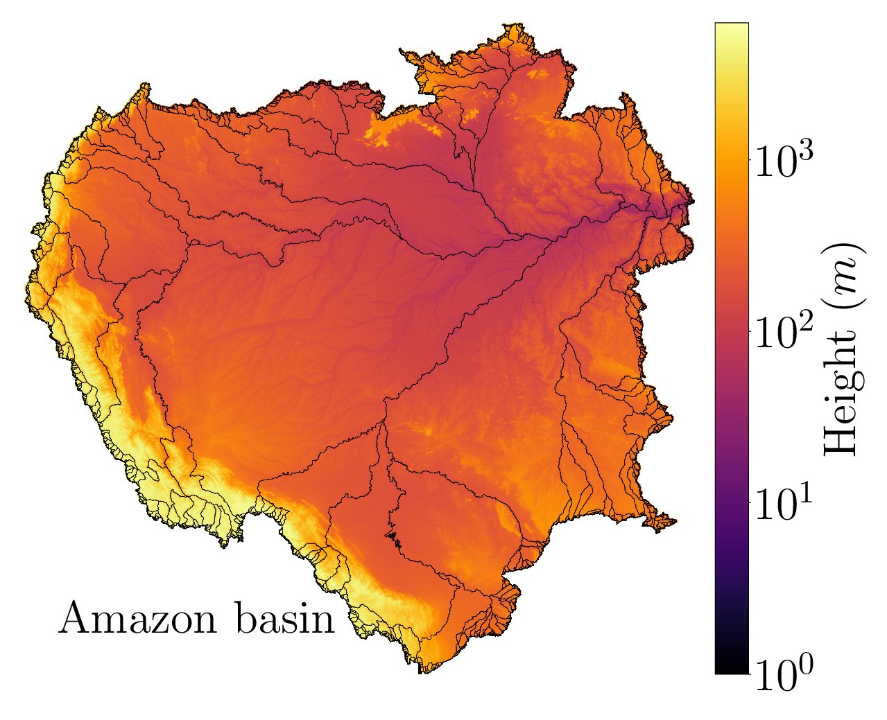 Figure 1
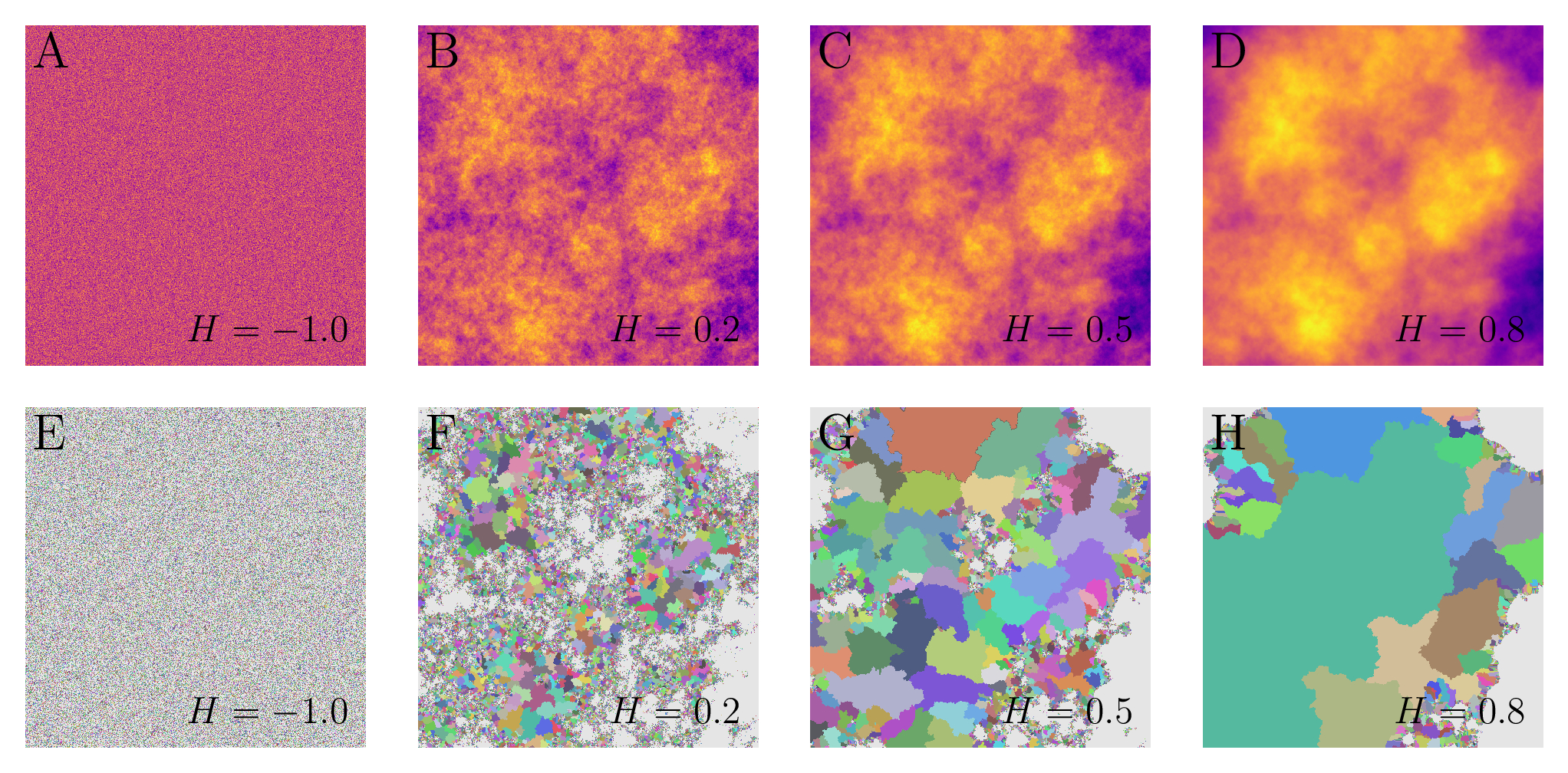 Figure 2
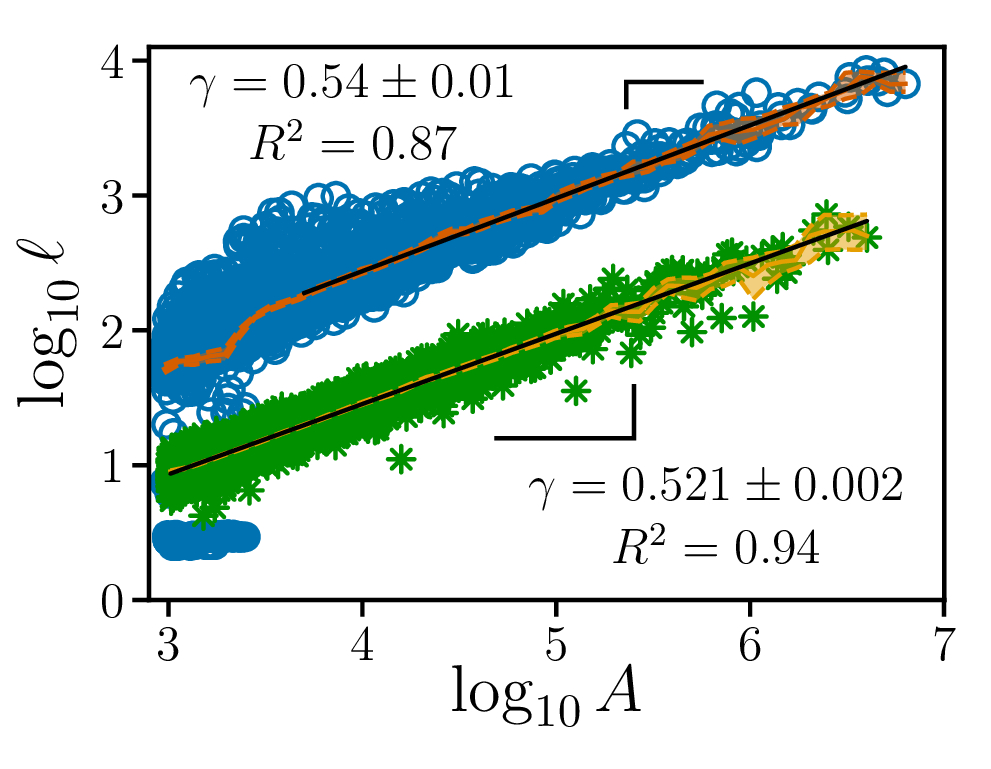 Figure 3
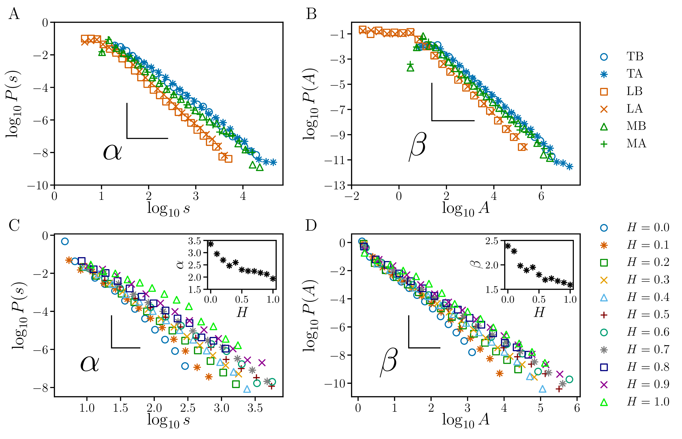 Figure 4
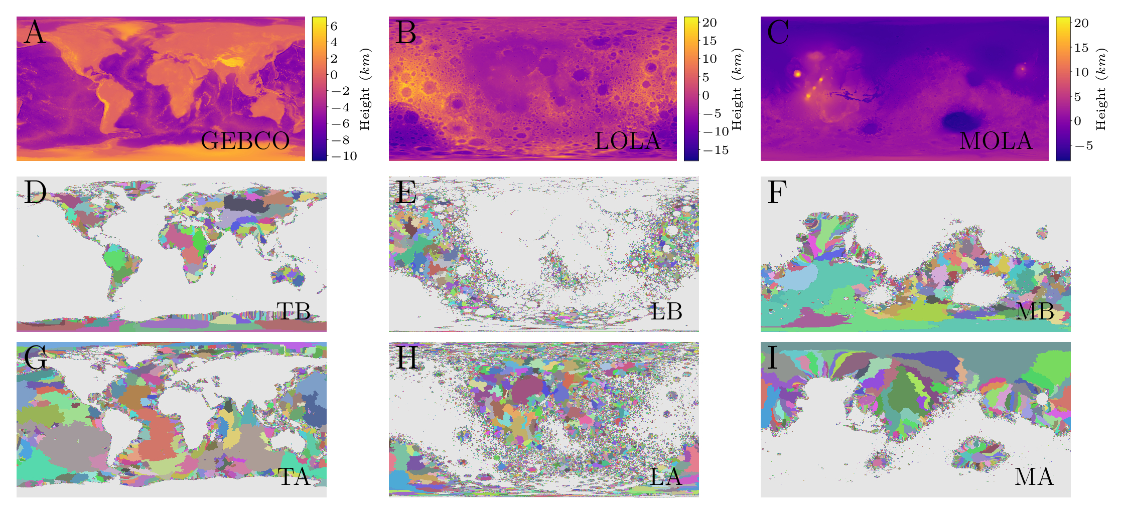 Figure 5
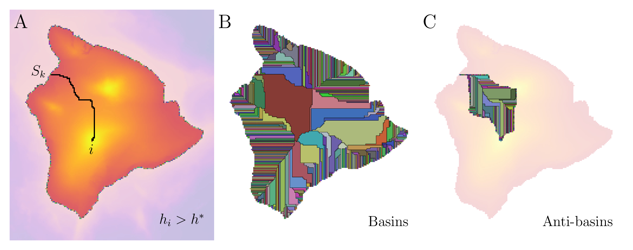 Figure 6
| Cases | Abbreviation | ||
|---|---|---|---|
| Terrestrial Basins | TB | 2.30 0.03 | 1.74 0.02 |
| Terrestrial Anti-basins | TA | 2.26 0.03 | 1.72 0.02 |
| Lunar Basins | LB | 2.70 0.02 | 1.93 0.01 |
| Lunar Anti-basins | LA | 2.64 0.04 | 1.89 0.02 |
| Martian Basins | MB | 2.33 0.04 | 1.75 0.02 |
| Martian Anti-basins | MA | 2.26 0.02 | 1.73 0.02 |
Peer Reviews
No public reviews on file for this paper yet. If you reviewed it on a platform where reviews are public (OpenReview, ICLR, NeurIPS, ICML), you can paste yours below so the community can read it here.
Videos
No videos yet. Explain this paper in a talk, walkthrough, or lecture? Add one.
A universal approach for drainage basins
Erneson A. Oliveira1,2,3111Correspondence to: [email protected], Rilder S. Pires3, Rubens S. Oliveira3, Vasco Furtado1, Hans J. Herrmann3,4,5, José S. Andrade Jr.3
1 Programa de Pós Graduação em Informática Aplicada, Universidade de Fortaleza, 60811-905 Fortaleza, Ceará, Brasil.
2 Mestrado Profissional em Ciências da Cidade, Universidade de Fortaleza, 60811-905 Fortaleza, Ceará, Brasil.
3 Departamento de Física, Universidade Federal do Ceará, Campus do Pici, 60451-970 Fortaleza, Ceará, Brasil.
4 PMMH, ESPCI, 7 quai St Bernard, 75005 Paris, France.
5 ETH Zürich, Computational Physics for Engineering Materials, Institute for Building Materials, Wolfgang-Pauli-Strasse 27, HIT, CH-8093 Zürich, Switzerland.
Abstract
Drainage basins are essential to Geohydrology and Biodiversity. Defining those regions in a simple, robust and efficient way is a constant challenge in Earth Science. Here, we introduce a model to delineate multiple drainage basins through an extension of the Invasion Percolation-Based Algorithm (IPBA). In order to prove the potential of our approach, we apply it to real and artificial datasets. We observe that the perimeter and area distributions of basins and anti-basins display long tails extending over several orders of magnitude and following approximately power-law behaviors. Moreover, the exponents of these power laws depend on spatial correlations and are invariant under the landscape orientation, not only for terrestrial, but lunar and martian landscapes. The terrestrial and martian results are statistically identical, which suggests that a hypothetical martian river would present similarity to the terrestrial rivers. Finally, we propose a theoretical value for the Hack’s exponent based on the fractal dimension of watersheds, . We measure for Earth, which is close to our estimation of . Our study suggests that Hack’s law can have its origin purely in the maximum and minimum lines of the landscapes.
Drainage Basins, Watersheds, River Networks, Invasion Percolation, Scaling Laws
I Introduction
Drainage basins play a fundamental role in the hydrologic cycle, which make them essential to diversity and maintenance of Life on Earth fetter2014 . The longstanding problem of characterising drainage basins has drawn much attention due to its importance in a variety of environmental issues, such as water management vorosmarty1998 ; knecht2012 ; brooks2012 , landslide and flood prevention dhakal2004 ; pradhan2006 ; lazzari2006 ; lee2006 ; yang2007 , and aquatic dead zones diaz2008 ; breitburg2018 ; goudie2018 . In this context, drainage basins, or simply basins, are all land areas sloping toward a single outlet, e.g. a river mouth or points of higher infiltration or evaporation rates. They are outlined by abstract boundary lines, called topographic divides or watersheds. The concept of watersheds appears in many other seemingly unrelated areas like percolation theory araujo2014 ; saberi2015 , image segmentation and medicine vincent1991 ; grau2004 ; ng2006 ; cousty2010 , and even international borders un1902 ; edaa2009 .
Watersheds are recognized as fractals in several cases breyer1992 ; fehr2009 ; fehr2011a ; fehr2011b , exhibiting self-similarity and a well defined fractal dimension. There are several objects that share the same fractal dimension of watersheds on uncorrelated random substrates (viz. ), such as optimal paths under strong disorder cieplak1994 ; cieplak1996 ; porto1997 ; porto1999 , minimum spanning trees on random networks dobrin2001 , backbones of the optimal path crack andrade2009 ; oliveira2011 ; andrade2011 , and bridge bonds on ranked surfaces shrenk2012 . All these loopless paths belong to the same universality class as watersheds. Furthermore, it is also known that watersheds are Schramm-Loewner evolution curves daryaei2012 and that it is possible to define hydrological watersheds burger2018 , where the infiltration process in the soil is taken into account.
The availability of digital elevation models (DEMs) allowed the development of modern techniques to automatically delineate watersheds. Nowadays, these methods are used in the standard Geographic Information System (GIS) software and are well established as a fundamental tool in Geoscience schwanghart2014 . The basic idea behind these methods is the calculation of the flow directions, which can be defined in several ways depending on the assumptions on the flow and number of neighbouring cells in the grid ocallaghan1984 ; freeman1991 ; quinn1991 ; costa-cabral1994 ; tarboton1997 ; peckham2007 ; gruber2009 ; shelef2013 . Simultaneously to the development of these methods, the concept of watersheds were also introduced in the context of contour delineation beucher1979 and became a widely used tool for image processing. The key difference among these methods is that those adopted in image processing do not use channels to define watershed lines. Instead, they simply search the landscape for the highest lines that divide it. In this context, even the most modern computational models are not able to get all watersheds of the globe at once, they are usually limited to specific regions. As compared to all these methods, methods based on invasion percolation as ours do not need to explore the entire space but only a fractal subset of it. Therefore, our method becomes more and more efficient the larger the landscape.
Here, we propose a simple model to fully delineate multiple drainage basins for any given landscape based on the traditional Invasion Percolation (IP) model wilkinson1983 , which is known to be a Self-Organized Criticality (SOC) model stauffer1994 , i.e. the IP model does not need a tuning parameter to evolve and identify the watershed. Our method allows us to study the morphological segmentation of global maxima and minima in image processing, even if the landscape stands for the gray scale of a brain Magnetic Resonance Imaging (MRI) or the heights of a celestial body with or without river channels. The novelty of our approach is to characterize all basins from a single height dataset through the definition of a reference (sea) level, i.e. our approach is free of parameter tuning.
II The Model
In 2009, Fehr et al. fehr2009 ; fehr2011a ; fehr2011b introduced a model, called Invasion Percolation-Based Algorithm (IPBA), in order to extract watersheds from landscapes. The IPBA was proposed for a regular square lattice of size with fixed boundary conditions in the vertical direction and periodic boundary conditions in the horizontal direction, where the height of each site was represented by . It was also defined that the upper and lower lines of the lattice represent the sinks of two basins, e.g. one at the North (N) and other at the South (S), respectively. In this context, the following rule for the identification of the basins was proposed: For each site , one applies the IP model, defining that the basin (N or S) to which the site belongs is the one that the IP invaded cluster reaches first. Thus, all sites of the lattice belong to one of the two basins and the interface line between them defines the watershed. To improve the computational performance of the task of finding the interface line, an efficient sweeping strategy was also introduced: (i) Initially, the sites are chosen along a straight line that connects the sinks. Therefore, when the IP processes from two neighbouring sites evolve to different sinks, a segment of the watershed lies between them. (ii) From then on, the sites are chosen only in the neighbourhood of the already known watershed segments in order to reveal more segments of the watershed, resulting at the end in the complete watershed. Fehr et al. fehr2009 also showed that the IPBA follows the same dynamics as the Vincent-Soille algorithm vincent1991 . The Vincent-Soille algorithm has a direct interpretation, which is basically a flooding process, although it is computationally inefficient. The main advantage of the IPBA is its computational performance, the IPBA presents a sublinear complexity time since it only explores a fractal subset of space of fractal dimension fehr2009 and this characteristic allows us to perform a global analysis to the drainage basins.
Our aim is to define a robust mathematical model for the delineation of multiple drainage basins through an extension of the IPBA. Suppose a regular rectangular lattice , where the height of each site is , analogous to the original model. We introduce a height threshold such that, if , then the th site belongs to a cluster, which we call height cluster, composed by all connected sites with height above that threshold. Otherwise, the th site does not belong to any cluster. As explained in the following section, we adopted throughout this study, which for Earth corresponds to sea level. For this particular choice, the height clusters define continents and islands on Earth, as shown in Fig. 1A. Here, the sinks () are all the border sites of the height clusters, i.e. the sea shore on Earth. Consequently, we know a priori that they define drainage basins separated by several interface lines, but their specific sizes and shapes need to be determined. Similarly to the ideas proposed by Fehr et al. fehr2009 , we define the following rule to identify basins present in the height clusters: The IP model is applied for each site defining that the basin () at which the site belongs is the one that the IP invaded cluster reaches first (see Fig. 1A). As depicted in Fig. 1B, the set of interface lines forms the watershed network that separates all basins in the height clusters. We also use a strategy analogous to the original IPBA to improve the performance of finding the watershed network. Here, the sweeping occurs in each basin as follows: (i) The sink defines the ends (initial and final segments) of its yet not identified watershed. (ii) For each basin, the sweeping occurs only at sites neighboring the already known watershed segments in order to reveal the missing ones. In other words, we scanned the sites along the watershed inner perimeter neighbourhood of each basin. This strategy drastically reduces the number of times that we need to apply the IP algorithm for the identification of the watershed network. (iii) Optionally, a simple burning algorithm can be applied to each basin in order to evaluate its area stauffer1994 .
Actually, we consider two versions of our algorithm along the study: A version with traditional periodic boundary conditions in horizontal direction and unconventional periodic boundary conditions in vertical direction for real landscapes, and another version with fixed boundary conditions on both directions for artificial landscapes. The unconventional periodic boundary conditions, adopted for real landscapes, are defined by imposing that each site in the top (bottom) row be neighbour of every other site in the top (bottom) row. These boundary conditions represent a mapping of a sphere into a lattice. They are needed because we performed all measures on the entire globe for real landscapes.
A natural extension of the watershed concept is the definition of its reciprocal line, called anti-watershed. The anti-watersheds are composed by lines of minimal heights, in contrast to the watersheds, defined in terms of lines of maximal heights. Therefore, if the basins can (grossly) be understood as “cavities” in a surface, then the anti-basins can also be understood as “humps” on that same (inverted) surface. We emphasize that anti-watersheds do not necessarily represent river channels, since a river channel (or a channel) is a “clearly defined watercourse (“natural or man-made channel through or along which water may flow”) which periodically or continuously contains moving water”, or is a “watercourse forming a connecting link between two water bodies”, or even is the “deepest portion of a watercourse, in which the main stream flows” wmo2012 , while a anti-watershed line may never contain any flowing water. Given an upside-down landscape, the same approach for watersheds can be considered to define the anti-watersheds. In this case, the watershed network represents the anti-watershed network in the original landscape. Furthermore, we can also define an anti-watershed network within a drainage basin (see Fig. 1C). Here, the lines of minimal heights represent the most deeper rivers and their tributaries in a lot of situations.
We highlight that our model just takes into account the drainage basins that flow out to the oceans, i.e. we are ignoring the endorheic drainage basins (or simply endorheic basins), which are those basins that flow out to any place other than the oceans, e.g. lakes or swamps, their amounts of water being balanced by infiltration or evaporation busby2012 . Nonetheless, we could also include such basins in our model introducing additional sinks (where and is the number of endorheic basins), located at the points of higher evaporation rates, for example. In this context, the total number of drainage basins () would depend on the spatial resolution of the data and the information available about the endorheic basins. Our code is available at https://github.com/erneson.
III Results
We applied the IPBA model to real and artificial landscapes in order to study the statistical properties of the drainage basins on Earth, Moon, and Mars. For real landscapes, we use three different DEMs throughout this study: the General Bathymetric Chart of the Oceans (GEBCO) gebco2014 , the Lunar Orbiter Laser Altimeter (LOLA) lola2014 , and the Mars Orbiter Laser Altimeter (MOLA) mola2014 . Such datasets consist of the map of heights for the Earth, Moon and Mars, respectively. Moreover, we obtained the artificial landscapes through the fractional Brownian motion (fBm) fisher1988 . We chose this method because we are interested in generating landscapes with tunable spatial long-range correlations since it is known that such correlations change the statistical properties of watersheds fehr2011b . We show all landscapes in Figs. 2A-C and Figs. 3A-D. We considered two scenarios for GEBCO, LOLA, and MOLA datasets: the original and the upside-down landscape orientations. We emphasize that we chose the GEBCO dataset to represent the terrestrial landscapes because it includes altimetric and bathymetric heights, which makes it more similar to LOLA and MOLA datasets. In other words, we used the GEBCO dataset in order to make a general and uniform comparison between Earth and two celestial bodies that do not have oceans (Moon and Mars). To perform a global analysis, the resolutions of the real datasets were decreased by a factor of , where is the resolution factor. Thus, each tile of sites was replaced by a single site with a value given by the mean of all original sites. The sizes of the used lattices were for GEBCO (original ), for LOLA (original ), and for MOLA (original ). For the fBm landscapes, we considered only the original orientation due to the natural symmetry of the Gaussian distribution used in the Ffm. In this case, we averaged our simulations over samples of lattices of for the traditional range of the Hurst exponent (). The following subsections show the corresponding results.
III.1 Real Landscapes
Here, we show the main results of our approach applied to real landscapes. In Figs. 2D and G, we show the results of our model applied to the original and upside-down landscapes of the Earth. In Figs. 2E, H, F, and I, we use the height threshold (hypothetical sea level) and perform the same analysis used for Earth’s landscape to obtain the basins and anti-basins for the Moon and Mars. We note that the basins and anti-basins look similar in the terrestrial and martian landscapes, while in the lunar landscape, they are affected by the impact basins, i.e. craters originated from the impact of asteroids. This similarity is quantified here through the statistical distributions of perimeters and areas of the basins and anti-basins for Earth, Moon and Mars. We included the lunar analysis as a counterpoint to show that the observed similarity between the terrestrial and Martian results is indeed genuine. The log-log plots of all these distributions shown in Figs. 4A-B clearly indicate the presence of long tails extending over several orders of magnitude. Moreover, these tails approximately follow power-law behaviors, and , for the perimeters and areas, respectively. By performing Ordinary Least Square (OLS) fits montgomery2006 to the corresponding distributions, we obtained estimates for the power-law exponents and that are summarized in Table 1. Similar results where found using a Maximum Likelihood Estimator (MLE) clauset2009 , as shown in the Supplementary Information (SI).
We found that the terrestrial and martian results are statistically identical, which suggests the surfaces of both planets underwent a similar formation history and that a hypothetical martian river would present some level of similarity to the terrestrial rivers, since both landscapes share the same statistics for watershed (maxima) and anti-watershed (minima) lines. There is already evidence that the Martian channels were formed by a series of fluvial and non-fluvial processes hargitai2018 . Furthermore, we found evidence that the obtained perimeter and area exponents are independent of the resolution factor (See SI). It is known that the effects of finite size are attenuated as the system size increases. We also obtained similar results for other values of on Earth, Moon and Mars.
In Fig. 5, we show the Amazon basin and its associated anti-basins defined by our algorithm on GEBCO dataset at the original resolution. In this special case, we are removing all internal sinks from the South American continent, i.e. we are allowing the existence of sites with negative heights within South America. We emphasise that several rivers (the deeper ones) follow the anti-watershed lines. The black lines in Fig. 5 stand for the anti-watershed network, which shows an impressive similarity with the Amazon river network (See SI for further comparisons). This similarity allows us to obtain the length of the longest river in a basin by approximating it by the length of the longest path from the point of minimal height (the mouth of the river) of the largest tree on the anti-watershed network. We defined the height of each point of the anti-watershed lines as the mean of the heights of its neighbouring sites. Therefore, we are ignoring any issues related to the initiation point of river channels wohl2017 . As a perspective for future work, quantitative analyses can be performed comparing the anti-watershed and river networks, e.g. see the proposed method by Grieve et al. grieve2016 .
We also performed the verification of Hack’s law rodriguez-iturbe2001 for the entire planet. This scaling law establishes the relation between the areas () of the basins and the maximum lengths () of their rivers, i.e.
[TABLE]
where is known as the Hack exponent. In Figure 6, we show Hack’s law for the original orientation of the terrestrial landscape considering only the basins with area greater than . We chose an area threshold to ensure that the analyzed basins were not too much affected by the resolution of the dataset. We found the Hack exponent with coefficient of determination , which is very close to our theoretical value of for Earth.
III.2 Artificial Landscapes
We applied the extension of the IPBA to artificial landscapes. In Figs. 3E-H, we show all basins defined by our model for the same samples presented in Figures 3A-D. As shown in Figures 4C and D, the perimeter and area distributions obtained from these landscapes are systematically affected by the presence of spatial correlations, quantified here in terms of the parameter . Moreover, except for the case of , all distributions generated from artificial landscapes can be approximately described by power laws, for perimeters, and for areas. For each value of , we averaged both distributions for all samples. The insets of the Figures 4C and D show that and decrease with the Hurst exponent . The exponents and range between and and between and , respectively. In the uncorrelated case (), however, we obtained less than one order of magnitude for and precluding the same kind of analysis.
In Fig. 6, we show Hack’s law obtained for (a close value of is usually obtained for real landscapes fehr2011b ), considering only the basins with area above . Such result led us to the following conjecture: Let the basin area be , the longest anti-watershed line be , and assuming that the anti-watershed lines are indeed watershed lines of the upside-down landscapes, it is known that , where is the linear length of the system and is the fractal dimension of the watershed lines fehr2009 . Since , we have:
[TABLE]
which gives . In other words, the Hack exponent depends on the fractal dimension of the anti-watershed lines. Fehr et al. fehr2011b showed that the fractal dimension of the watersheds decreases with the Hurst exponent , similarly to the Optimal Path Cracks oliveira2011 , and the coastlines on correlated landscapes morais2011 . The fractal dimension of the watershed lines ranges between and , what gives to the Hack exponent a corresponding range from to . For real landscapes, the fractal dimensions of the watershed lines are around ( for the Alps fehr2009 , for the Himalaya fehr2009 , and for the Andes fehr2011b ). Therefore, our expected Hack exponent for Earth should be , a value which is in good agreement with the result shown in Fig. 6 ( with coefficient of determination for artificial landscapes). This result suggests that Hack’s law, often observed for river networks, is an intrinsic effect of topography, i.e. it depends, in essence, on the watershed and anti-watershed lines. In other words, Hack’s law may have a purely geometrical origin and does not depend on physical laws governing the water flow on a surface birnir2008 .
IV Discussion
We proposed a general model to fully delineate multiple drainage basins for any given landscape of heights through an extension of the IPBA. The novelty of our approach is to characterise all basins from a single height dataset through the definition of a reference (sea) level. Such fact allows us to claim that our model is free of parameter tuning. In this way, we are able to delineate the basins through the definition of the watershed network (maximal lines of a landscape) as well as the anti-basins through the definition of the anti-watershed network (minimal lines of a landscape). In order to show that our algorithm was robust, we applied it to real and artificial landscapes. In both cases, we found that the perimeter and area distributions are ruled by power laws with exponents and , respectively. It was also shown that the terrestrial and martian results are statistically identical, which suggests that the surfaces of Earth and Moon have undergone similar formation processes and that a hypothetical martian river would present similarity to the terrestrial rivers, since both landscapes share the same statistics for watershed and anti-watershed networks. We also verified that, in the Amazon basin and its associated anti-basins defined by our approach, several rivers (the most deeper ones) rest on anti-watershed lines. Furthermore, we showed that the exponents and , for artificial landscapes, decrease systematically with the Hurst exponent and that they are invariant under the inversion of real landscapes. Finally, we found a theoretical value for the Hack’s exponent based on the fractal dimension of the watershed and anti-watershed lines, . We measured for artificial landscapes with and for Earth, which agree within error bars with our estimation of for real cases.
V Methods
V.0.1 Real Landscapes
We use three different DEM datasets throughout this study. The first dataset is the General Bathymetric Chart of the Oceans (GEBCO) gebco2014 consisting of altimetric and baltimetric heights, i.e. the heights above and below the sea level, around the Earth globe. The resolution of this dataset is () in both coordinates, equivalent to a square lattice with edge length of at the Equator line. The other two are the Lunar Orbiter Laser Altimeter (LOLA) lola2014 and Mars Orbiter Laser Altimeter (MOLA) mola2014 consisting of the map of heights for the Moon and Mars, respectively. The LOLA resolution is about , while MOLA resolution is , both in relation to their corresponding “Equator”. We show the three datasets in Figs. 2A-C. In addition, we point out that all datasets are freely available and are friendly ready-to-use, i.e. all technical preprocessing steps were already performed by the GEBCO, LOLA, and MOLA research teams. We do not perform any additional preprocessing (such as any hydrologic correction or void filling), except the addition of a tiny noise in the heights (, much less than the precision of all datasets) in order to ensure that all values in real landscapes are different, defining a unique sequence if the height values are sorted.
We also emphasise that all three datasets are available in the Geographic Coordinate System (GCS), more precisely, in latitude and longitude grids in the image format TIFF, i.e. they are mapped on spheres, the terrestrial (with radius ), the lunar (with radius ), and the martian (with radius ). For GEBCO, the reference surface (the zero height) is defined by the terrestrial geoid. The geoid is the natural shape that a static fluid would present due to the gravitational potential of its celestial body schubert2007 . On Earth, the oceans could be considered static and, consequently, they are well approximated by such a surface. For LOLA and MOLA, the geoid concept is generalised by the gravitational equipotential surface with the mean lunar and martian radius at the Equator, respectively, defining hypothetical sea levels lola2014 ; mola2014 . We adopt the height threshold for all landscapes in order to make a general comparative analysis.
Here, we perform the calculation of the area of each site by the composition of two spherical triangles (the site areas for artificial landscapes have no unit of measure and are all unitary). The area of a spherical triangle with edges , and is given by todhunter1863 ,
[TABLE]
where , , , and . In this formalism, is the sphere radius, where, in our case, , and the edge lengths are calculated by the great circle (geodesic) distance between two points and on the sphere surface given by the Haversine formula snyder1987 :
[TABLE]
where and . The values of () and (, measured in radians, are the longitude and latitude, respectively, of the point (). Therefore, we are able to define the site areas, and, consequently, obtain the total area of a given basin, since each basin is composed by a set of sites.
V.0.2 Artificial Landscapes
We obtained artificial landscapes through the fractional Brownian motion (fBm) fisher1988 in order to study the watershed and anti-watershed networks. One of the most established method to generate a fBm is the so-called Fourier filtering method (Ffm) fisher1988 . The basic idea of the Ffm is to define random Fourier coefficients in the reciprocal space, distributed according to the following power-law spectral density:
[TABLE]
where is the frequency of the dimension , is the topological dimension, and is the spectral exponent. Subsequently, the inverse Fourier transform is applied to generate a correlated distribution in the real space. In our case , the correlated distribution is a landscape. Each landscape is characterised by an exponent , called Hurst exponent, related to the spectral exponent by . Four cases can be distinguished: (i) For , the uncorrelated landscape (see Fig. 3A). (ii) For , the landscape has a negative correlation, i.e. the increments are anticorrelated (see Fig. 3B). (iii) For , the landscape is correlated, but the increments are uncorrelated (see Fig. 3C), which is the case of the classical Brownian motion fisher1988 . (iv) Finally, for , the landscape has a positive correlation, i.e. the increments are correlated (see Fig. 3D).
VI Acknowledgements
We gratefully acknowledge CNPq, CAPES, FUNCAP and the National Institute of Science and Technology for Complex Systems in Brazil for financial support.
VII Author contributions statement
E.A.O., H.J.H., and J.S.A. designed research; E.A.O., R.S.P., and R.S.O. performed research; E.A.O., R.S.P. and J.S.A. analyzed data; and E.A.O., R.S.P., R.S.O., V.F., H.J.H., and J.S.A. wrote the paper. All authors reviewed the manuscript.
VIII Data Availability
All data used in this manuscript are free available. Please, check the references related to GEBCO, LOLA, and MOLA datasets.
IX Additional information
IX.1 Competing interests
We declare we have no competing interests.
The reference list from the paper itself. Each links out to its DOI / PubMed record.
- 1(1) Fetter, C.W. Applied Hydrogeology (Pearson Education Limited, 2014).
- 2(2) Vörösmarty, C.J., Federer, C.A. & Schloss, A.L. Potential evaporation functions compared on US watersheds: Possible implications for global-scale water balance and terrestrial ecosystem modeling. J. Hydrol. 207 , 147–169 https://doi.org/10.1016/S 0022-1694(98)00109-7 (1998). · doi ↗
- 3(3) Knecht, C.L., Trump, W., ben Avraham, D. & Ziff, R.M. Retention capacity of random surfaces. Phys. Rev. Lett. 108 , 045703 https://doi.org/10.1103/Phys Rev Lett.108.045703 (2012). · doi ↗
- 4(4) Brooks, K.N., Ffolliott, P.F. & Magner, J.A. Hydrology and the management of watersheds (Wiley-Blackwell, 2012).
- 5(5) Dhakal, A.S. & Sidle, R.C. Distributed simulations of landslides for different rainfall conditions. Hydrol. Process. 18 , 757–776 https://doi.org/10.1002/hyp.1365 (2004). · doi ↗
- 6(6) Pradhan, B., Singh, R.P. & Buchroithner, M.F. Estimation of stress and its use in evaluation of landslide prone regions using remote sensing data. Adv. Space Res. 37 , 698–709 https://doi.org/10.1016/j.asr.2005.03.137 (2006). · doi ↗
- 7(7) Lazzari, M., Geraldi, E., Lapenna, V. & Loperte, A. Natural hazards vs human impact: an integrated methodological approach in geomorphological risk assessment on the Tursi historical site, Southern Italy. Landslides 3 , 275–287 https://doi.org/10.1007/s 10346-006-0055-y (2006). · doi ↗
- 8(8) Lee, K.T. & Lin, Y.T. Flow analysis of landslide dammed lake watersheds: a case study. J. Am. Water Resour. Assoc. 42 , 1615–1628 https://doi.org/10.1111/j.1752-1688.2006.tb 06024.x (2006). · doi ↗