Rotational Surfaces with second fundamental form of constant length
Alexandre P. Barreto, Francisco Fontenele, Luiz Hartmann

TL;DR
This paper classifies complete rotational surfaces in three-dimensional space with a second fundamental form of constant length, identifying a family of such surfaces and characterizing the only embedded examples as spheres and cylinders.
Contribution
It introduces an infinite family of non-embedded rotational surfaces with constant-length second fundamental form and characterizes all complete rotational surfaces with this property.
Findings
Complete non-embedded rotational surfaces with constant second fundamental form form an infinite family.
Complete embedded rotational surfaces with this property are only spheres and cylinders.
The classification includes a unique family up to homothety and rigid motions.
Abstract
We obtain an infinite family of complete non embedded rotational surfaces in whose second fundamental forms have length equal to one at any point. Also we prove that a complete rotational surface with second fundamental form of constant length is either a round sphere, a circular cylinder or, up to a homothety and a rigid motion, a member of that family. In particular, the round sphere and the circular cylinder are the only complete embedded rotational surfaces in with second fundamental form of constant length.
Click any figure to enlarge with its caption.
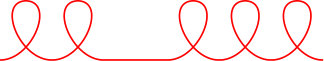 Figure 1
 Figure 2
 Figure 3
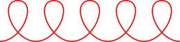 Figure 4
 Figure 5
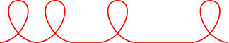 Figure 6
 Figure 7
Peer Reviews
No public reviews on file for this paper yet. If you reviewed it on a platform where reviews are public (OpenReview, ICLR, NeurIPS, ICML), you can paste yours below so the community can read it here.
Videos
No videos yet. Explain this paper in a talk, walkthrough, or lecture? Add one.
Taxonomy
TopicsGeometric Analysis and Curvature Flows · Point processes and geometric inequalities · Geometric and Algebraic Topology
Rotational Surfaces with second fundamental form
of constant length
Alexandre Paiva Barreto
Departamento de Matemática, Universidade Federal de São Carlos (UFSCar), Brasil
,
Francisco Fontenele
Departamento de Geometria, Universidade Federal Fluminense (UFF), Brasil.
and
Luiz Hartmann
Departamento de Matemática, Universidade Federal de São Carlos (UFSCar), Brasil
[email protected] http://www.dm.ufscar.br/profs/hartmann
Abstract.
We obtain an infinite family of complete non embedded rotational surfaces in whose second fundamental forms have length equal to one at any point. Also we prove that a complete rotational surface with second fundamental form of constant length is either a round sphere, a circular cylinder or, up to a homothety and a rigid motion, a member of that family. In particular, the round sphere and the circular cylinder are the only complete embedded rotational surfaces in with second fundamental form of constant length.
Key words and phrases:
Rotational surface; length of the second fundamental form; Weingarten surface.
2010 Mathematics Subject Classification:
Primary 53A05, 53C42 ; Secondary 53C40, 14Q10.
All authors are partially supported by CNPq(Brasil)
Contents
- 1 Introduction
- 2 Convexity of the profile curves
- 3 Phase portrait of the fundamental vector field
- 4 *Proof of Theorem *1.1
1. Introduction
A surface in the -dimensional Euclidean space is called a Weingarten surface if there exists some relation
[TABLE]
among its principal curvatures and . Since the principal curvatures of a surface can always be determined from its mean curvature and its Gaussian curvature , and vice-versa, the relation (1.1) can always be rewritten as a relation .
Weingarten surfaces is a classical topic in Differential Geometry that began with the works of Weingarten in the middle of the 19th century **[20, 21]** and that has been a subject of interest for many authors since then (see Chern **[2]**, Hartman and Winter **[7]**, Hopf **[8]**, Voss **[19]**, Rosenberg and Sá Earp **[18]**, Kühnel and Steller **[11]**, López **[12, 13, 14, 15]**, to name just a few).
Minimal surfaces, surfaces with constant mean curvature and surfaces with constant Gaussian curvature are classical examples of Weingarten surfaces. Another well known class (generalizing the previous ones) is that of the linear Weingarten surfaces, i.e., Weingarten surfaces verifying either the relation
[TABLE]
or the relation
[TABLE]
where are constants such that and do not vanish simultaneously.
The complete classification of Weingarten surfaces is far from being achieved. The existent results deal mostly with the linear case, sometimes making use of additional topological/geometric hypothesis and/or working with important subclasses of surfaces such as revolution surfaces **[8, 14, 11, 18]**, tubes along curves and cyclic surfaces **[13, 15]**, ruled surfaces and helicoidal surfaces **[10]**, translation surfaces **[3, 16]**, etc. In general, the approaches used to treat the linear case do not apply to the non-linear case. Therefore, results concerning non-linear Weingarten surfaces are more rare **[18, 11]**.
In this paper we study rotational surfaces in the -dimensional Euclidean space whose second fundamental forms have constant length (recall that the squared length of the second fundamental form of a surface in is defined as the trace of , where is its shape operator). In other words, we study rotational Weingarten surfaces that satisfy the non-linear relation
[TABLE]
or equivalently
[TABLE]
for some .
In this case we prove the following result (notice that since the property of having constant is invariant by homotheties in , we can assume without loss of generality that ):
Theorem 1.1**.**
*There are two infinite families and of complete non embedded rotational surfaces in with . The family is one parameter and its members are periodic surfaces, while the members of are surfaces. Moreover, any complete rotational surface with is either a round sphere of radius , a circular cylinder of radius 1 or, up to a rigid motion in , a member of one of the two families. *
Corollary 1.2**.**
The only complete embedded rotational -surfaces in with second fundamental form of constant length are the round sphere and the circular cylinder.
Non trivial examples of compact surfaces (embedded or immersed) with second fundamental form of constant length are unknown by the authors. In view of Theorem 1.1 and Corollary 1.2, one can then formulate the following question:
Question 1.3**.**
- Is there a compact surface, other than the round sphere, embedded/immersed in the Euclidean 3-space whose second fundamental form has constant length?
It is worth to point out that the above question has a negative answer in the class of the compact surfaces with positive Gaussian curvature **[1, Theorem 5 on p. 347 and Section 4]** (see also **[9]** or **[5, Theorem 2.3]**).
The importance of the class of hypersurfaces whose second fundamental forms have constant length goes beyond the context of Weingarten surfaces. We mention **[4]** (see also **[6]**), where it is proved that the generalized cylinders are the only complete embedded self-shrinkers in with polynomial volume growth whose second fundamental forms have constant length.
The paper is organized as follows. In Section 2, we prove that the profile curve of any rotational surface in with is convex, i.e., its signed curvature does not change signal. This fact enable us to reduce the study of rotational surfaces with to the study of the trajectories of a certain vector field in the plane. The study of this vector field is made in Section 3. Finally, we prove Theorem 1.1 in Section 4.
Acknowledgments
The authors would like to thank Thiago de Melo (IGCE-UNESP) for helpful conversations during the preparation of this work and for his help with the figures.
2. Convexity of the profile curves
Our goal in this section is to prove that the profile curve of any rotational -surface , whose shape operator has length , is convex. By applying a rigid motion of if necessary, we can assume that is contained in the -plane and that the axis of revolution is the -axis.
Let , be a parametrization of such that and for all , and let be a continuous (and, hence, of class ) function satisfying
[TABLE]
It is easy to see that the function satisfying Eq. (2.1) is unique up to an integer multiple of . The principal curvatures of are given by (see e.g., **[14]**)
[TABLE]
Since by hypothesis, one then has
[TABLE]
As we observed in the introduction, the proof of Theorem 1.1 will be based on a careful study of the trajectories of a suitable vector field in the plane. The fundamental property of the profile curves that makes this approach possible is provided by the following proposition (recall that the signed curvature of is ):
Proposition 2.1**.**
The function is monotone.
Before proceeding to the proof of Proposition 2.1, let us explain how to relate profile curves with the trajectories of a specific vector field.
Let and be as above. Assuming that is monotone, reparametrizing we can assume that . Then, by Eq. (2.1) and (2.3),
[TABLE]
Let be the (smooth) vector field defined by
[TABLE]
where . As long as , the system in Eq. (2.4) can be rewritten as
[TABLE]
and so the curve is a trajectory of . A representation of and the vector field can be seen in Figure 1.
Conversely, given a trajectory of and , consider the curve where
[TABLE]
Using Eq. (2.2), (2.5) and (2.6) one easily proves that the surface in obtained by the rotation of the image of around the -axis satisfies .
In the proof of Proposition 2.1, as well as in the proofs of later results, we will use the following technical lemma. In its statement, and are as in the beginning of this section.
Lemma 2.2**.**
For any , the following assertions hold:
- (i)
* if, and only if, and .* 2. (ii)
If then . 3. (iii)
If , then there exists such that , .
- Proof.
(i) If then, by Eq. (2.3), the function attains a maximum at . Hence,
[TABLE]
Since , one obtains from the above equality and Eq. (2.1) that
[TABLE]
Using this information in Eq. (2.3), one concludes that . The converse is an immediate consequence of Eq. (2.3).
(ii) From Eq. (2.3) and one obtains
[TABLE]
and so
[TABLE]
The conclusion now follows by taking square roots in the above inequality.
(iii) Supposing, by contradiction, that the conclusion does not hold, we have for some sequence that converges to . Since, by (i), for all , passing to a subsequence and reparametrizing if necessary, one can assume that , for all .
We claim that
[TABLE]
Indeed, if for some then, since and for all , there is such that
[TABLE]
Hence, . On the other hand, from (i), (ii) and Eq. (2.8) one obtains . This contradiction proves Eq. (2.7).
By (i), (ii) and Eq. (2.7),
[TABLE]
Then, by Eq. (2.7) and ,
[TABLE]
Since by (i), we have two possibilities:
a) , for some .
b) , for some .
Assuming a), from Eq. (2.10) one obtains
[TABLE]
Then, by the first inequality of Eq. (2.9),
[TABLE]
From Eq. (2.7), (2.10), (2.11) and (ii), we obtain
[TABLE]
Hence, for fixed , we have
[TABLE]
and so
[TABLE]
It now follows from Eq. (2.11) and the fact that the cosine function is decreasing on , that
[TABLE]
Since, by Eq. (2.3) and (2.11), , inequalities Eq. (2.7) and (2.12) imply
[TABLE]
contradicting the fact, easily verified, that , for all .
A reasoning entirely similar to the above shows that b) cannot occur either. Hence, on a neighbourhood of . ∎
Proof of Proposition 2.1:* Suppose, by contradiction, that is not monotone. Then there exists in such that either i) or ii) below holds:*
i) and .
ii) and .
Assuming i), we have
[TABLE]
Define
[TABLE]
Since attains a local maximum at and at , we have . Then, by Lemma 2.2 (i), and . The latter implies that either or , for some . If , one has , such that
[TABLE]
Then, , for all , contradicting Lemma 2.2 (iii).
If , there exists such that
[TABLE]
Then, , for all , which also contradicts Lemma 2.2 (iii).
A reasoning entirely similar to the above shows that ii) can not occur either. Hence, the function is monotone.∎
3. Phase portrait of the fundamental vector field
With the aim to prove Theorem 1.1, we study in this section the trajectories of the vector field defined by Eq. (2.5). This study will be carried out through a series of technical lemmas.
Since the trajectories of are invariant by horizontal translations by multiples of (that is, if is a trajectory of then so is the curve for any ), it is sufficient to consider the trajectories that pass through some point such that .
Lemma 3.1**.**
Let be a point in such that and . If is the maximal integral curve of satisfying , then there exists such that .
- Proof.
We can assume that , for otherwise the conclusion follows immediately from . Suppose, by contradiction, that the conclusion does not hold. Then, by the definition of ,
[TABLE]
and so
[TABLE]
Let
[TABLE]
By Eq. (3.1) and (3.2), and . From the maximality of and the fact that has no singularities in , one obtains , and so
[TABLE]
We have two cases to consider:
i) (and so ).
ii) (and so ).
Since the vectors of on the boundary of points inward, we can use transversality to conclude that case i) can not occur. However, we will discard this case by a direct argument. Consider the (positive) function defined by . By Eq. (3.3) and (3.4),
[TABLE]
Using now Eq. (2.4), (3.3) and (3.4), one obtains
[TABLE]
Then, there is such that and so
[TABLE]
Letting in the above inequality, and using Eq. (3.5), one obtains
[TABLE]
contradicting the fact that , for all .
Suppose now ii). From Eq. (3.2) and Lemma 2.2 (ii), we obtain for all , and so
[TABLE]
for every . Taking the limit when in the above inequality, and using Eq. (3.3) and b), we obtain
[TABLE]
and thus . Choosing such that
[TABLE]
one has, since the cosine function is decreasing on ,
[TABLE]
Then, by Eq. (2.3) and the above inequality,
[TABLE]
and so . Using now that for every , one concludes that . Hence, by Eq. (3.6) and (3.7),
[TABLE]
which is obviously false. This contradiction finishes the proof of the lemma. ∎
Lemma 3.2**.**
Let such that . If is the maximal integral curve of satisfying , then there exists such that .
- Proof.
Assuming, by contradiction, that the conclusion does not hold, one has , and so
[TABLE]
Let such that (such a number exists by Lemma 3.1). Since is bounded above and, by Eq. (2.4) and (3.8),
[TABLE]
one concludes that . Then, since , one also has that is bounded. Hence, converges to a point in when , but this can not occur because (see, for instance, [17, p. 91]). ∎
Lemma 3.3**.**
Given and , let be the maximal integral curve of satisfying . Then, and for every , where denotes the reflection in with respect to the line . In short, is symmetric with respect to the line .
- Proof.
Consider the curve defined by
[TABLE]
It is easy to see that is an integral curve of . Since , it follows from the maximality of that and
[TABLE]
∎
Lemmas 3.2 and 3.3 tell us that to obtain a picture of the phase portrait of it is sufficient to consider the family of trajectories , where is the maximal integral curve of such that .
From Lemma 3.2 and the fact that is positive on , one concludes, for each , that the trajectory either crosses the ray or converges to a point when . Moreover, each point such that is the limit point of some . The later is clear when and , as the vector field can be continuously extended, without singularities, to a neighbourhood of , and follows easily for the other two values of by a continuity argument.
The following lemma shows that two distinct trajectories of the family can not converge to the same point in . Note that this fact does not follow from the standard theory of ordinary differential equations, because the vector field does not admit a differentiable extension to a neighbourhood of any given point in .
Lemma 3.4**.**
With the same notation as above, assume for some that
[TABLE]
Then (and hence ).
- Proof.
Assume, by contradiction, that , say . Setting and , from Eq. (3.10) one obtains that (respectively, ) is a diffeomorphism from (respectively, ) to . Let . By the Chain Rule and the Inverse Function Theorem,
[TABLE]
Since and for , we have and so
[TABLE]
for all . Using this inequality in Eq. (3.11), we obtain
[TABLE]
Using again the equality , it follows from the Change of Variables Formula that
[TABLE]
for every . Hence, by Eq. (3.12),
[TABLE]
Taking the limit when , and using Eq. (3.10), one obtains , contradicting our assumption . Hence . ∎
4. Proof of Theorem 1.1
As before, for each denote by the maximal integral curve of such that . From Lemma 3.4 and the discussion that precedes its statement one concludes that there is a unique such that when . Moreover, when , the trajectory either crosses the ray or converges to a point in depending on whether or (see Figure 2).
For each , consider the curve defined by , where
[TABLE]
and the surface of obtained by the rotation of the image of around the -axis. As we have seen in Section 2, the length of the shape operator of equals 1 at every point. The detailed classification of the surfaces reads:
Theorem 4.1**.**
Let be as above.
(i) If then is a complete -surface. Moreover, is periodic and has self-intersections.
(ii) is incomplete, but it can be extended in infinite many ways to a complete -surface satisfying . Any such extension has self-intersections.
(iii) is the sphere with center at and radius (minus two points).
(iv) If or then is incomplete and cannot be extended to a surface with .
Concerning the Gaussian curvature of the surfaces obtained in the above theorem, we observe that the only surfaces with positive Gaussian curvature are the surfaces with . For all the others, the Gaussian curvature changes the signal.
Theorem 4.1 is a direct consequence of the following result:
Theorem 4.2**.**
Let be as above.
(i) If then and is of class . Moreover, is periodic and has self-intersections.
(ii) and can be extended in infinite many ways to a profile curve of class defined on . Any such extension has self-intersections.
(iii) is a parametrization by arc length of the semicircle in the -plane with center at and radius .
(iv) If or then and cannot be extended to a profile curve defined on an open interval containing properly.
- Proof.
(i) From and the discussion in the beginning of this section one infers that there exists such that . Applying Lemma 3.3 with and one concludes that . Being the trajectory of a vector field of class , , and hence , is of class .
We will now prove that is periodic. Since, by Eq. (2.5) and Lemma 3.3, the maps and are both trajectories of passing through , one has
[TABLE]
On the other hand, by Eq. (4.1) one has
[TABLE]
Since by Eq. (4.2), it follows that
[TABLE]
Since for all by Eq. (4.2), the curve is periodic.
To complete the proof of (i), it remains to show that is non-embedded. In fact, we will show that the restriction of to the interval has already self-intersections. For that observe first that, since , and , the function is a diffeomorphism from to . In particular, there exists a unique such that . Let be defined by
[TABLE]
Clearly, is a diffeomorphism, and . Moreover,
[TABLE]
and
[TABLE]
[TABLE]
Since, by Eq. (2.4),
[TABLE]
one then has
[TABLE]
Using the informations collected above, we will now compare the values of for , and . Since for , from Eq. (4.1) we obtain
[TABLE]
On the other hand, by Eq. (4.6), (4.7) and (4.9), one has
[TABLE]
Hence, by Eq. (4.1) and inequality above,
[TABLE]
The curve is symmetric with respect to the line . Indeed, by Lemma 3.3 one has
[TABLE]
and so
[TABLE]
for every .
Since on and, by Eq. (4.10) and (4.12), , there exists a unique such that . Then, by Eq. (4.14),
[TABLE]
Since by Eq. (4.13), it follows that . Hence, the restriction of to the interval has a self-intersec-tion.
(ii) We begin by showing that . Let such that . For every we have
[TABLE]
where in the last inequality we used the fact that and the cosine function is nonnegative on .
Claim**.**
There is such that
[TABLE]
Indeed, since and when , from Eq. (2.4) we obtain
[TABLE]
Then, again by Eq. (2.4),
[TABLE]
and so
[TABLE]
From Eq. (2.4) and the above equality one obtains
[TABLE]
Therefore,
[TABLE]
and the claim follows.
From Eq. (4.16) and (4.17), we obtain
[TABLE]
Setting , one has
[TABLE]
Using this information in Eq. (4.22), we obtain
[TABLE]
for every . Therefore, .
In order to prove that can be extended to a profile curve of class defined on , we need to evaluate the limits of and when . From Eq. (2.4) one obtains, after some work,
[TABLE]
Since , and when , it follows from Eq. (4.20) and (4.24) that
[TABLE]
As to , observe that, since , , and , the derivatives of either of the last two terms on the right hand side of Eq. (4.24) goes to zero when . Therefore,
[TABLE]
where in the last equality we used Eq. (4.19). Since, by Eq. (2.4),
[TABLE]
one has
[TABLE]
The first term on the right hand side goes to zero by Eq. (4.19) and (4.27). Hence,
[TABLE]
Using Eq. (2.4) again, one obtains
[TABLE]
It now follows from Eq. (4.26), Eq. (4.29) and the above equality that
[TABLE]
It is possible to extend gluing together copies of . By Eq. (4.18), (4.25) and (4.30), this extension is (at least) (recall that if a profile curve is of class then its corresponding angle function is of class ). Another way to extend is gluing together copies of and horizontal segments with any length and with height equal to 1. By the same equations, these extensions are but not (see Figure 3, items (B), (C) and (D), for a sample of these extensions).
To complete the proof of (ii), it remains to show that any extension of is non-embedded. But clearly this follows from the fact that has a self-intersection, which in turn can be proved as in (i) (with playing the role of ).
(iii) As can be easily seen, the curve
[TABLE]
is a trajectory of . Since , one has . Then, by Eq. (4.1),
[TABLE]
which is a parametrization by arc length of the portion of the circle in the -plane with center and radius that is above the -axis.
(iv) Let . Since and, by item (iii), when , it follows from Lemma 3.4 that and either or .
Suppose, by contradiction, that . Since when and either or , there exist and such that
[TABLE]
Then, by Eq. (2.1),
[TABLE]
for every , a contradiction. Hence, .
Suppose, by contradiction, that can be extended to a profile curve where , say. Let be a function satisfying
[TABLE]
Since for all , and, by Eq. (4.1),
[TABLE]
one concludes that and the restriction of to the interval differ by an integer multiple of . Assuming without loss of generality that , one has
[TABLE]
and
[TABLE]
which contradicts Lemma 2.2 (i) as . ∎
Now we finish the prove of our main theorem.
Completion of proof of Theorem 1.1:* Let and , , be as in the beginning of this section, and let . Let be the set of extensions of constructed in the proof of Theorem 4.2 (ii), and the (infinite) family of surfaces obtained by the rotation of the images of the curves in around the -axis. By Theorem 4.1 (i), the surfaces in have the properties stipulated in the statement of the theorem. That the surfaces in also meet the stipulated conditions is a consequence of the proof of Theorem 4.2 (ii). This establishes the first part of the theorem.*
Let be a complete rotational surface of class satisfying . Applying a rigid motion if necessary, we can assume that its axis of revolution is the -axis and that its profile curve is contained in the -plane. Let , , be a parametrization of such that and for all . Let be a -function such that
[TABLE]
As we have seen in Section 2, the function satisfies
[TABLE]
If is constant, by the above equality one has that is constant. Then and so . Being complete, is then a right circular cylinder of radius 1.
Suppose now that is not constant. Since is monotone by Proposition 2.1, reparametrizing if necessary we can assume that for all . Let such that . Without loss of generality, we can assume that . Let be the maximal interval containing on which . As we have seen in Section 2, the map is an integral curve of the vector field defined by Eq. (2.5). By the results in Section 3, there is a unique trajectory in the family that passes through . Let such that . Assuming without loss of generality that , it follows from the maximality of that . Write and consider its associated profile curve ( cf. the beginning of this section). Since
[TABLE]
it holds that
[TABLE]
for some .
Claim.* and .*
Assuming, by contradiction, that , one has . Then, since on and ,
[TABLE]
From the above inequality and definition of one obtains . It now follows from Eq. (4.31) that can be extended to an interval containing properly, contradicting the completeness of . This contradiction proves that . In the same way, one proves that .
It follows from the Claim that . Indeed, if we had , reasoning as above one would obtain . On the other hand, from one would obtain , a contradiction. In the same manner, one proves that . Hence and, by Eq. (4.31),
[TABLE]
for some .
From Eq. (4.32) one obtains that either or . In fact, if we had or , from Theorem 4.2 (iv) we would obtain that is a translation of , and so would be incomplete, contradicting the hypothesis.
In the case , it follows from Eq. (4.32) and Theorem 4.2 (i) that for all , and therefore (up to translation).
In the case , it follows from Eq. (4.32) and Theorem 4.2 (iii) that . Since is complete, one concludes that is, up to translation, the sphere with center at and radius .
*Finally, consider the case . By Eq. (4.32), is an extension of . Since is complete and, by Theorem 4.1 (ii), is incomplete, one has and . We will conclude that, up to congruence, belongs to the family and so . For that we can assume that is not identically zero on , for otherwise outside and the conclusion holds trivially. We claim that for any at which , there is an open interval of length containing such that differs from the image of by a horizontal vector. We will prove the claim in the case (the proof in the case is analogous). Denote by the maximal interval containing on which . By what we have already proved ( cf. Eq. (4.32)), coincides with a horizontal translation of the image of , for some . Since and (by Lemma 2.2(i), since ), we have and the claim is proved. Let be subintervals of such that and are both horizontal translations of the image of . If the distance between and is positive but less than , then, by the previous claim, one has , and hence , in the interval between and . It is now clear that the image of is made up of curves congruent to and eventually of horizontal segments of height equal to
- Therefore, and so .∎*
The reference list from the paper itself. Each links out to its DOI / PubMed record.
- 1[1] A. D. Alexandrov, Uniqueness theorems for surfaces in the large I-V , Amer. Math. Soc. Trans. Ser. (2) 21 (1962), 341–416.
- 2[2] Shiing-shen Chern, Some new characterizations of the Euclidean sphere , Duke Math. J. 12 (1945), 279–290. MR 0012492
- 3[3] Franki Dillen, Wendy Goemans, and Ignace Van de Woestyne, Translation surfaces of Weingarten type in 3-space , Bull. Transilv. Univ. Braşov Ser. III 1(50) (2008), 109–122. MR 2478011
- 4[4] Qi Ding and Y. L. Xin, The rigidity theorems of self-shrinkers , Trans. Amer. Math. Soc. 366 (2014), no. 10, 5067–5085. MR 3240917
- 5[5] F. Fontenele and Sérgio L. Silva, Sharp estimates for the size of balls in the complement of a hypersurface , Geom. Dedicata 115 (2005), 163–179. MR 2180046
- 6[6] Qiang Guang, Self-shrinkers with second fundamental form of constant length , Bull. Aust. Math. Soc. 96 (2017), no. 2, 326–332. MR 3703914
- 7[7] Philip Hartman and Aurel Wintner, Umbilical points and W 𝑊 W -surfaces , Amer. J. Math. 76 (1954), 502–508. MR 0063082
- 8[8] Heinz Hopf, Über Flächen mit einer Relation zwischen den Hauptkrümmungen , Math. Nachr. 4 (1951), 232–249. MR 0040042