The Ostrovsky Hunter equation with a space dependent flux function
Neelabja Chatterjee, Nils Henrik Risebro

TL;DR
This paper investigates the periodic Ostrovsky-Hunter equation with a spatially dependent flux, establishing existence, uniqueness, and convergence of entropy solutions via finite volume schemes with a specific convergence rate.
Contribution
It proves the existence and uniqueness of entropy solutions for the spatially dependent flux case and demonstrates convergence of finite volume approximations at rate 1/2.
Findings
Existence and uniqueness of entropy solutions for the equation.
Finite volume scheme converges to the entropy solution at rate 1/2.
The flux function's regularity is crucial for the analysis.
Abstract
We study the periodic Ostrovsky-Hunter equation in the case where the flux function may depend on the spatial variable. Our main results are that if the flux function is twice differentiable, then there exists a unique entropy solution. This entropy solution may be constructed as a limit of approximate solutions generated by a finite volume scheme, and the finite volume approximations converge to the entropy solution at a rate 1/2.
Click any figure to enlarge with its caption.
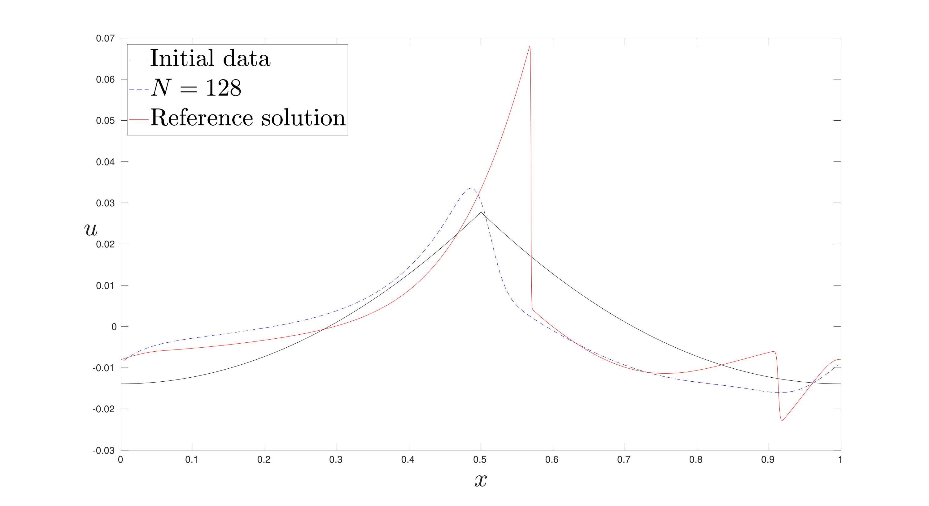 Figure 1
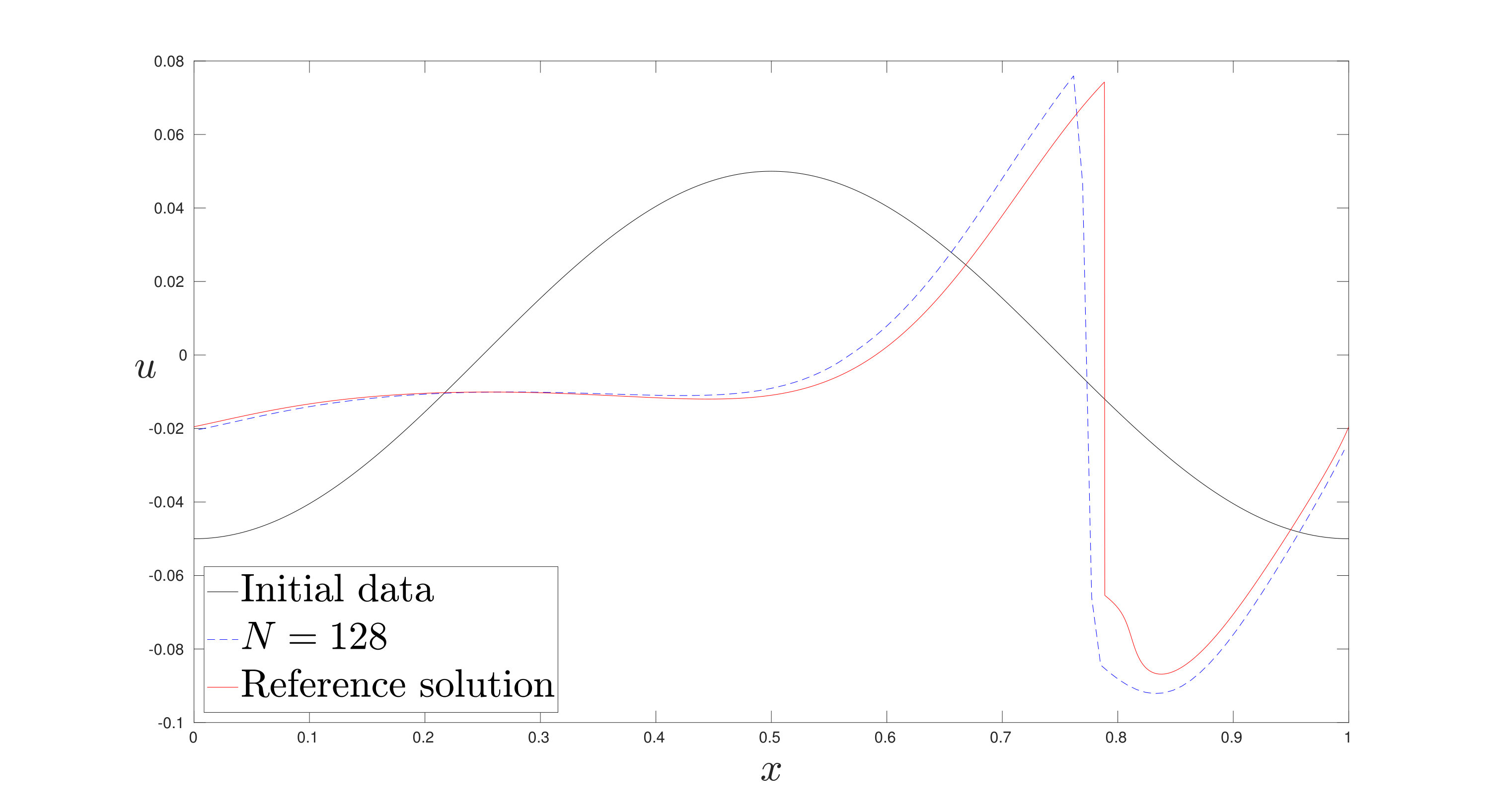 Figure 2
Peer Reviews
No public reviews on file for this paper yet. If you reviewed it on a platform where reviews are public (OpenReview, ICLR, NeurIPS, ICML), you can paste yours below so the community can read it here.
Videos
No videos yet. Explain this paper in a talk, walkthrough, or lecture? Add one.
Taxonomy
TopicsStochastic processes and financial applications · Mathematical Biology Tumor Growth · advanced mathematical theories
The Ostrovsky-Hunter
equation with a space dependent flux function
N. Chatterjee
Department of mathematics
University of Oslo
P.O. Box 1053, Blindern
N–0316 Oslo, Norway
and
N. H. Risebro
Department of mathematics
University of Oslo
P.O. Box 1053, Blindern
N–0316 Oslo, Norway
Abstract.
We study the periodic Ostrovsky-Hunter equation in the case where the flux function may depend on the spatial variable. Our main results are that if the flux function is twice differentiable, then there exists a unique entropy solution. This entropy solution may be constructed as a limit of approximate solutions generated by a finite volume scheme, and the finite volume approximations converge to the entropy solution at a rate .
Key words and phrases:
Ostrovsky-Hunter equation, short-pulse equation,Vakhenko equation, space dependent flux function, stability, numerical method, stability, uniqueness
2010 Mathematics Subject Classification:
Primary: 35L35, 65M06; Secondary: 45M33
This project has received funding from the European Union’s Horizon 2020 research and innovation programme under the Marie Skłodowska-Curie grant agreement No 642768.
1. Introduction
To model small-amplitude long waves in a rotating fluid of finite depth, Ostrovsky [1] derived the following non-linear evolution equation
[TABLE]
where and are real constants and . Here denotes the amplitude of waves, while and are the space and time variables respectively. The equation can be formally deduced using two asymptotic expansions of the shallow water equations, once with respect to the rotation frequency and then with respect to the amplitude of the waves, see [2]. Later, in a study of long internal waves in a rotating fluid Hunter [2], investigated the limit of no high-frequency dispersion . This formally reduces to the Ostrovsky-Hunter (OH) equation:
[TABLE]
The OH equation also arises as a model of high frequency waves in a relaxing medium, see [3]. In both cases .
Equation (1.2) can also be derived by including the effects of background rotation in the shallow water equation, and then using singular perturbation methods, see [6, 7]. In this context, it is worth mentioning that equation (1.1) generalizes the KdV equation, which corresponds to . The equation (1.2) is also known as the reduced Ostrovsky equation [1, 8, 10], short wave equation [2], Ostrovsky-Vakhnenko equation [11, 12], or Vakhnenko equation [4, 5, 9]. Also, equation (1.1) is used to model ultra short light pulses in silica optical fibres [13, 14, 15, 20], in which case . In this case (1.1) is sometimes referred to as the “short-pulse-equation”.
In this context we note that Hunter established the connection between the KdV equation and short wave equation (1.2), see [2], as the no-rotation and no-long wave dispersion limits of the same equation. But in the case of oceanic waves near the shore, the waves usually propagate on a background whose properties vary. In such a variable medium the linear phase speed of the wave, which is encoded in the flux term (instead of ) has spatial dependency. To model such scenario the variable coefficient KdV equation was derived by Johnson [23] for water waves and by Grimshaw [24] for internal waves (see also [25] for a review). Motivated by this, in this paper we aim to design and analyze a numerical scheme for the OH equation with spatial dependency in the flux.
As is commonly done, we rewrite the OH equation (1.2) as the following system
[TABLE]
Without loss of generality, we can set , and will in the sequel do so. Since is defined as any anti-derivative of , we need an additional constraint to close the system. This can be done in different ways, see [18, 19, 21]. We shall adopt the approach in [22], where we study the problem (1.2) in a periodic setting . In this case it is natural to redefine the right hand side by subtracting the (constant) term . This has the attractive side effect of conserving , i.e.,
[TABLE]
if satisfies the zero mean condition . This condition was also assumed to hold initially in [14, 2]. So the equation we are studying in this paper reads
[TABLE]
where is periodic with period , and . Note that since satisfies the zero mean condition, is also periodic. This is essentially an extension of the system studied in [22] to the case where is allowed to depend on the spatial variable . As in [22], discontinuites in will develop independently of the smoothness of the initial data, so that (1.3) must be interpreted in the weak sense. Furthermore, as with scalar conservation laws, in order to show well posedness, we shall consider entropy solutions.
Our main results are as follows. Assuming that the mapping is uniformly Lipschitz continuous locally in , and that the initial data are of bounded variation and satisfy the zero mean condition, we have that
[TABLE]
where and are entropy solutions with initial data and respectively. Furthermore, we establish convergence to the unique entropy solution of approximate solutions generated by an upwind scheme. We also prove a Kuznetsov-type lemma, see [26], satisfied by the entropy solution, and this lemma allows us to conclude that the approximate solutions converge at the rate in .
The rest of this paper is organized as follows. In Section 2 we detail precise definitions and assumptions and notation, as well as the definition of the finite volume scheme. In Section 3 we prove the necessary bounds which imply that the approximate solutions form a strongly compact family in . Furthermore, we prove that the approximate solutions satisfy an entropy inequality, and this is used to show that any limit of the approximate solutions is an entropy solution. In Section 4 we establish a “Kuznetsov type lemma” enabling us to compare exact entropy solutions with arbitrary functions. Then this comparison result is used to show that the approximate solutions “converge at a rate”. Finally, in Sections 5 we exhibit some concrete numerical results.
2. Preliminaries and notation
The problem we study is the following
[TABLE]
Regarding the initial data we shall assume that
[TABLE]
The flux function is assumed to be in , which in particular implies that it is Lipschitz continuous in and locally Lipschitz continuous in . Since solutions of (2.1) generically develop discontinuities, solutions must be considered in the weak sense. A function in is a weak solution of (2.1) if
[TABLE]
For all test functions which are -periodic in . Here . Let , following [22] we define entropy solutions as
Definition 1** (Entropy Solution).**
A function is called an entropy solution of the Ostrovsky-Hunter Equation (2.1), if for all constants the following inequality holds
[TABLE]
for all non-negative test functions which are -periodic in the variable. Here and are defined as the Kružkov entropy and entropy flux respectively,
[TABLE]
Throughout this paper we employ the following convention, and denote the partial derivatives of with respect to and respectively. If is differentiable, then we have
[TABLE]
Furthermore, we use the convention that denotes a generic positive constant, whose actual value may change from one occurrence to the next.
In order to define the numerical scheme, set
[TABLE]
where and are positive integers, and . We also define for , for and for . We also define the intervals for and . In order to define a piecewise constant approximations, set .
Next we define the finite volume approximation. Let be a numerical flux which is monotone and consistent, i.e.,
[TABLE]
In addition we assume that is differentiable in and that both and are Lipschitz continuous in and .
We can now define the finite volume scheme. Set , and let be defined by
[TABLE]
for and . Here
[TABLE]
where we use periodic boundary conditions and . The term is defined as
[TABLE]
Finally we define the initial values by
[TABLE]
Observe that since is assumed to be of bounded variation,
[TABLE]
The spatial discretization and the temporal are related through a CFL-condition. Consider the map
[TABLE]
We choose so small that for all , is non-decreasing in all its arguments. For this monotonicity to hold it is sufficient to choose
[TABLE]
where is a constant depending on (through ).
It is also useful to define
[TABLE]
where and are any sequences. With this notation the scheme can be written
[TABLE]
Using (2.4) we see that , and that it is consistent to define and . With this convention we also have that
[TABLE]
We also observe that
[TABLE]
so that if , then also
[TABLE]
Defining , we can estimate as
[TABLE]
We shall often use the short hand notations , and .
3. Discrete estimates and convergence
In this section our aim is to prove the compactness of our scheme using Kolmogorov’s compactness theorem. To employ this theorem we require a supremum bound, a bound and an continuity-in-time bound on the approximate solutions, all of which are uniform in the discretization variable .
For simplicity of exposition, we shall show such estimates in the case where . This means that , which is non-decreasing in . The proof in the general case then follows mutatis mutandi.
Lemma 2** (-bound).**
The solution of the scheme (2.3) satisfies the following bound
[TABLE]
Proof.
Using the monotonicity of
[TABLE]
The result follows by an application of Gronwall’s inequality. ∎
Now in the next lemma we are going to obtain a uniform bound on total variation in space for the numerical solutions.
Lemma 3** ( bound).**
The solution of the scheme (2.3) satisfies the bound
[TABLE]
where is a positive constant depending on and its first and second derivatives.
Proof.
Assume that satisfies
[TABLE]
where is a given function and . Using the monotonicity of we find that
[TABLE]
and similarly
[TABLE]
Subtracting, we find that
[TABLE]
with
[TABLE]
This implies
[TABLE]
Regarding the “” term
[TABLE]
where
[TABLE]
This gives
[TABLE]
Now we set , then and . Furthermore,
[TABLE]
Then we get the bound
[TABLE]
The estimate (3.1) follows after applying Lemma 2 and then Gronwall’s inequality. ∎
Next, we show a so-called “discrete entropy inequality”.
Lemma 4**.**
For all and all constants , we have
[TABLE]
Proof.
Choose , and in (3.2) and (3.3), the results are
[TABLE]
with
[TABLE]
Note that , multiplying the first inequality with and the second with , where is the Heaviside function, yields
[TABLE]
Add these and divide by , then rearrange and divide by to get (3.5). ∎
Lemma 5** (Time continuity bound).**
For all we have that
[TABLE]
where is a constant depending on and its derivatives.
Proof.
Using in (3.4), we find that and . Thus
[TABLE]
Multiplying with and using the bound and Lemma 2, we get
[TABLE]
We use Gronwall’s inequality to conclude the proof. ∎
Note that our assumptions on and the initial data imply that
[TABLE]
for some constant depending on .
Next we define the piecewise constant approximation by
[TABLE]
With these three bounds, Lemmas 2, 3, 5, we can apply Helly’s theorem, [17, Theorem A.11], to prove that is compact.
Lemma 6** (Compactness lemma).**
Let be the family obtained from the scheme (2.3) with chosen such that is monotone for all and for all . Then the exists a sequence with as , and a function such that in .
Now we can use the discrete entropy condition (3.5) to show that any limit satisfies the entropy condition (2.2).
Theorem 7**.**
Assume that the initial data satisfies the zero mean condition , and that satisfies (2.6) (so that is monotone). Then is an entropy solution according to Definition 1.
Proof.
For simplicity we write for . Choose a non-negative, -periodic test function and set . Let , multiply the discrete entropy inequality (3.5) with , and sum by parts in and to obtain
[TABLE]
where
[TABLE]
Using similar arguments to those that can be found in the proof of the analogous result in [22], it is straightforward to show that we can let in (3.9) to conclude that satisfies (2.2). The proof of this uses in particular that
[TABLE]
and that both and are consistent and Lipschitz continuous in both and . ∎
4. A Kuznetsov type lemma, stability and convergence rate
As in [22] the similarity of the OH equation to a scalar conservation law allows us to estimate the -difference between the an entropy solution and other functions which are not necessarily solutions of (2.1). In this section we establish such a comparison result and use it to prove that the approximations defined by the finite volume scheme (2.3) – (2.5) converge to an entropy solution as .
4.1. A comparison result
For any function define
[TABLE]
where and are defined in Definition 1 and . Choose the test function
[TABLE]
where and are standard mollifiers, with being extended periodically outside the interval . Let and put in and integrate in and . This defines the following functional
[TABLE]
For any function , we define the moduli of continuity
[TABLE]
Remark 8**.**
From the proofs of Lemmas 2, 3, and 5 if follows that
[TABLE]
[TABLE]
In this setting, we have the following version of the Kuznetsov lemma.
Lemma 9**.**
Let be an entropy solution of the Ostrovsky-Hunter equation with the associated initial data . Then for any the following estimate holds
[TABLE]
where is a constant depending on , , and its first derivatives.
Proof.
For simplicity we write for . Using that , and that , we add and to compute
[TABLE]
As is standard for scalar conservation laws, see e.g., [17], the terms (4.4) – (4.7) can be estimated to yield the terms containing the initial and final data, plus the term starting with “” in (4.2). The term (4.8) can be overestimated as in [22] by
[TABLE]
The term (4.3) can by estimated as in [16] by
[TABLE]
Collecting these bounds
[TABLE]
The proof is concluded by applying Gronwall’s inequality. ∎
If is another entropy solution with initial data (satisfying the zero mean condition), then , and we can send and to zero in (4.2) to prove the following.
Theorem 10**.**
If and are entropy solutions of the Ostrovsky-Hunter equation (2.1) with initial data and respectively, then
[TABLE]
Observe that since the entropy solution is unique, then the whole sequence , rather than only a subsequence, converges.
4.2. Convergence rate
We can use Lemma 9 with to measure the error of the finite volume scheme.
Lemma 11**.**
Let be the entropy solution to (2.1) and let be the piecewise constant interpolation defined by (3.8), where is obtained by the scheme (2.3) – (2.5). Assume that is in , and that is locally bounded, -periodic and twice continuously differentiable. Then there exists a constant , depending on , and , but not on , or , such that
[TABLE]
Proof.
Again we write , after summation by parts we find that
[TABLE]
where is defined in (4.1) and
[TABLE]
Next, multiply the discrete entropy inequality (3.5) by and sum over and to get
[TABLE]
Write , so that . Then
[TABLE]
We need to bound . The integral of the first term on the right can be bounded as follows,
[TABLE]
where we have used (3.6) and (3.7). The terms (4.11) and (4.12) can be bounded similarly,
[TABLE]
Next, we consider (4.13), we split this into a sum of two terms
[TABLE]
The second of these can be bounded by summation by parts,
[TABLE]
The first integral of the first term of this expression can be estimated as
[TABLE]
The bound on the second term is identical. To bound we must bound the integral of the last term,
[TABLE]
To bound the integral of we use the continuity of and the observation that
[TABLE]
which implies that
[TABLE]
for some . Therefore
[TABLE]
Hence
[TABLE]
The term (4.14) is bounded in [22, Section 6.2] as
[TABLE]
The last term, the integral of (4.15), can be bounded using the Lipschitz continuity of ,
[TABLE]
The proof is concluded by collecting the bounds on the integrals of all the terms (4.10) – (4.15). ∎
From Lemma 11 it easily follows that converges at a rate .
Theorem 12**.**
Let and be as in Lemma 11. then
[TABLE]
where is a constant independent of .
Proof.
This result follows by setting in (4.9). We have that is defined in (2.5), therefore since is in . To conclude the proof apply Lemma 9, and recall that for , all moduli of continuity are uniformly linear in the last argument. ∎
5. Numerical examples
In this section we complement our theoretical results by two numerical experiments. Both experiments use the flux function
[TABLE]
As far as we know, with given above, there are no solutions to (2.1) in closed form. When measuring the accuracy of the approximations, we therefor use an approximation generated by the finite volume scheme with a small . We used the Engquist-Osher numerical flux
[TABLE]
Our first example uses initial data that coincides with those of the so-called “corner wave”. This is a closed form solution of the OH-equation with , but not so in our case. This corner wave initial data is given by
[TABLE]
Figure 1 shows the initial data, as well as the approximate solutions at , with and the reference solution using for .
The second example uses smoother initial data
[TABLE]
and Figure 2 shows the approximations for , and .
We observe that although the data are smooth, the solution seems to have a discontinuity.
By running the scheme with different , we can try to estimate the convergence rate numerically. In Table 1 we show the relative -errors, defined by
[TABLE]
We have done this for both examples, and as a reference solution, , we used the finite volume approximation with .
We observe that the convergence rates are higher that the theoretically proven rate. Although we are measuring “self-convergence”, it may well be the case that when the solution is a smooth as our examples seem to show (continuously differentiable except for a single discontinuity), the actual convergence rate is higher than .
The reference list from the paper itself. Each links out to its DOI / PubMed record.
- 1[1] Ostrovsky, L.A. Nonlinear internal waves in a rotating ocean . Okeanologia. 18, 119–125 (1978).
- 2[2] Hunter, J. Numerical solutions of some nonlinear dispersive wave equations. Computational solution of nonlinear systems of equations (Fort Collins, CO, 1988) Lectures in Appl. Math. 26, Amer. Math. Soc., Providence, RI, 301–316, 1990.
- 3[3] Vakhnenko, V.O. Solitons in a nonlinear model medium . J. Phys. A Math. Gen. 25, 4181–4187 (1992).
- 4[4] Morrison, J.A.; Parkes, E.J.; and Vakhnenko, V.O. The N loop soliton solutions of the Vakhnenko equation . Nonlinearity. 12(5):1427–1437, 1999.
- 5[5] Parkes, E. J. and Vakhnenko, V. O. The calculation of multi-soliton solutions of the Vakhnenko equation by the inverse scattering method . Chaos, Solitons and Fractals. 13(9):1819–1826, 2002.
- 6[6] di Ruvo, L. Discontinuous solutions for the Ostrovsky-Hunter equation and two-phase flows . Ph D thesis, University of Bari (2013).
- 7[7] Hunter, J. and Tan, K.P. Weakly dispersive short waves . Proceedings of the I Vth international Congress on Waves and Stability in Continuous Media (1987).
- 8[8] Parkes, E.J. Explicit solutions of the reduced Ostrovsky equation . Chaos Solitons Fractals. 31, 602–610 (2007).