Dilute Fermi gas at fourth order in effective field theory
C. Wellenhofer, C. Drischler, A. Schwenk
TL;DR
This paper computes the complete fourth-order term in the Fermi-momentum expansion for a dilute Fermi gas's ground-state energy using effective field theory, and compares its convergence with quantum Monte-Carlo results.
Contribution
It provides the first calculation of the fourth-order term in the Fermi-momentum expansion for dilute Fermi gases using effective field theory.
Findings
The expansion converges well for |k_F a_s| ≤ 0.5.
Comparison with quantum Monte-Carlo results confirms the convergence.
First complete fourth-order calculation in this context.
Abstract
Using effective field theory methods, we calculate for the first time the complete fourth-order term in the Fermi-momentum or expansion for the ground-state energy of a dilute Fermi gas. The convergence behavior of the expansion is examined for the case of spin one-half fermions and compared against quantum Monte-Carlo results, showing that the Fermi-momentum expansion is well-converged at this order for .
Click any figure to enlarge with its caption.
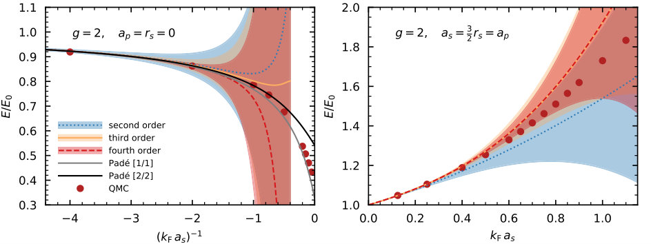 Figure 1
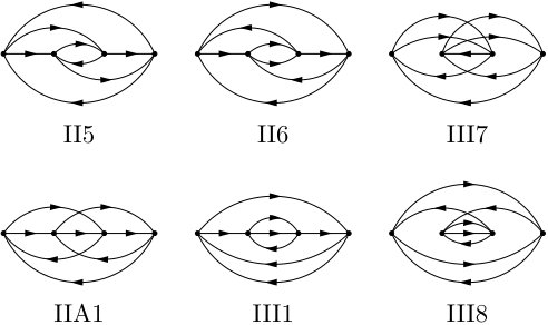 Figure 2
| diagram | factor | value |
|---|---|---|
| I1∗ | ||
| I2∗+I3+I4∗+I5∗ | ||
| I6 | ||
| IA1 | ||
| IA2 | ||
| IA3 | ||
| II1∗+II2∗ | ||
| II3+II4 | ||
| II5∗∗ | ||
| II6∗∗,∗ | ||
| II7+II12 | ||
| II8+II11 | ||
| II9 | ||
| II10 | ||
| IIA1∗∗ | ||
| IIA2+IIA4 | ||
| IIA3 | ||
| IIA5 | ||
| IIA6 | ||
| III1∗∗∗,∗∗,∗+III7+III8∗∗∗,∗ | ||
| III2∗∗∗+III9+III10∗∗∗ | ||
| (II5+IIA1)g=2 | ||
| (II6+III1+III7+III8) | ||
Peer Reviews
No public reviews on file for this paper yet. If you reviewed it on a platform where reviews are public (OpenReview, ICLR, NeurIPS, ICML), you can paste yours below so the community can read it here.
Videos
No videos yet. Explain this paper in a talk, walkthrough, or lecture? Add one.
Dilute Fermi gas at fourth order in effective field theory
C. Wellenhofer
Institut für Kernphysik, Technische Universität Darmstadt, 64289 Darmstadt, Germany
ExtreMe Matter Institute EMMI, GSI Helmholtzzentrum für Schwerionenforschung GmbH, 64291 Darmstadt, Germany
C. Drischler
Department of Physics, University of California, Berkeley, CA 94720, United States of America
Lawrence Berkeley National Laboratory, Berkeley, CA 94720, United States of America
A. Schwenk
Institut für Kernphysik, Technische Universität Darmstadt, 64289 Darmstadt, Germany
ExtreMe Matter Institute EMMI, GSI Helmholtzzentrum für Schwerionenforschung GmbH, 64291 Darmstadt, Germany
Max-Planck-Institut für Kernphysik, Saupfercheckweg 1, 69117 Heidelberg, Germany
Abstract
Using effective field theory methods, we calculate for the first time the complete fourth-order term in the Fermi-momentum or expansion for the ground-state energy of a dilute Fermi gas. The convergence behavior of the expansion is examined for the case of spin one-half fermions and compared against quantum Monte-Carlo results, showing that the Fermi-momentum expansion is well-converged at this order for .
The dilute Fermi gas has been a central problem for many-body calculations for decades Lenz (1929); Lee and Yang (1957); de Dominicis and Martin (1957); Efimov (1965); Amusia and Efimov (1965); Baker (1965); Efimov (1966); Amusia and Efimov (1968); Baker (1971); Bishop (1973); Lieb et al. (2005). Renewed interest in this problem has been triggered by striking progress with ultracold atomic gases. In particular, by employing so-called Feshbach resonances Chin et al. (2010) one can tune inter-atomic interactions and thereby probe Fermi systems over a wide range of many-body dynamics Bloch et al. (2008). On the theoretical side, a systematic approach towards the dynamics of fermions (or bosons) at low energies has emerged in the form of effective field theory (EFT) Hammer and Furnstahl (2000); Steele ; Furnstahl et al. (2001); Furnstahl and Hammer (2002); Schäfer et al. (2005); Hammer and König (2017). Motivated by this, we revisit the expansion in the Fermi momentum of the ground-state energy density of a dilute gas of one species of interacting fermions. Using perturbative EFT methods, we calculate up to fourth order in the expansion, including for the first time the complete fourth-order term. From this, we analyze the convergence behavior of the expansion, and obtain precise predictions for with systematic uncertainty estimates. Our analytic results have important applications for various problems in many-body physics, including benchmarks for experimental and theoretical studies of cold atoms, the construction of improved models of neutron star crusts, and for constraining nuclear many-body calculations at low densities.
Short-ranged EFT represents a systematic framework for the dynamics of fermions (or bosons) at low momenta , where denotes the breakdown scale. At low momenta, details of the underlying interactions are not resolved and can be replaced by a series of contact interactions. Few- and many-body observables are then expressed in terms of a systematic expansion in (called “power counting”). The EFT Lagrangian is given by the most general operators consistent with Galilean invariance, parity, and time-reversal invariance. The low-energy constants of the Lagrangian have to be fitted to experimental data or (if possible) can be matched to the underlying theory. Assuming spin-independent interactions, the (unrenormalized) Lagrangian reads (see, e.g., Refs. Steele ; Hammer and Furnstahl (2000); Furnstahl et al. (2001); Furnstahl and Hammer (2002); Schäfer et al. (2005); Hammer and König (2017))
[TABLE]
where are nonrelativistic fermion fields, \mathchoice{\vbox{\halign{#\cr\leftrightarrowfill@{\scriptstyle}\crcr\nointerlineskip\cr\hfil\displaystyle\nabla\hfil\crcr}}}{\vbox{\halign{#\cr\leftrightarrowfill@{\scriptstyle}\crcr\nointerlineskip\cr\hfil\textstyle\nabla\hfil\crcr}}}{\vbox{\halign{#\cr\leftrightarrowfill@{\scriptscriptstyle}\crcr\nointerlineskip\cr\hfil\scriptstyle\nabla\hfil\crcr}}}{\vbox{\halign{#\cr\leftrightarrowfill@{\scriptscriptstyle}\crcr\nointerlineskip\cr\hfil\scriptscriptstyle\nabla\hfil\crcr}}}=\mathchoice{\vbox{\halign{#\cr\leftarrowfill@{\scriptstyle}\crcr\nointerlineskip\cr\hfil\displaystyle\nabla\hfil\crcr}}}{\vbox{\halign{#\cr\leftarrowfill@{\scriptstyle}\crcr\nointerlineskip\cr\hfil\textstyle\nabla\hfil\crcr}}}{\vbox{\halign{#\cr\leftarrowfill@{\scriptscriptstyle}\crcr\nointerlineskip\cr\hfil\scriptstyle\nabla\hfil\crcr}}}{\vbox{\halign{#\cr\leftarrowfill@{\scriptscriptstyle}\crcr\nointerlineskip\cr\hfil\scriptscriptstyle\nabla\hfil\crcr}}}-\mathchoice{\vbox{\halign{#\cr\rightarrowfill@{\scriptstyle}\crcr\nointerlineskip\cr\hfil\displaystyle\nabla\hfil\crcr}}}{\vbox{\halign{#\cr\rightarrowfill@{\scriptstyle}\crcr\nointerlineskip\cr\hfil\textstyle\nabla\hfil\crcr}}}{\vbox{\halign{#\cr\rightarrowfill@{\scriptscriptstyle}\crcr\nointerlineskip\cr\hfil\scriptstyle\nabla\hfil\crcr}}}{\vbox{\halign{#\cr\rightarrowfill@{\scriptscriptstyle}\crcr\nointerlineskip\cr\hfil\scriptscriptstyle\nabla\hfil\crcr}}} is the Galilean invariant derivative, h.c. the Hermitian conjugate, and the fermion mass.
The ultraviolet (UV) divergences that appear beyond tree level in perturbation theory can be regularized by introducing a cutoff for relative momenta and Jacobi momenta . The two- and three-body potentials emerging from are then given by
[TABLE]
Perturbative renormalization is carried out by introducing counterterms such that the divergent contributions are canceled. In the two-body sector, this leads to
[TABLE]
where the cutoff-dependent parts are counterterms. For the renormalized two-body potential the residual cutoff dependence due to terms in perturbation theory vanishes in the limit . Matching the two-body low-energy constants to the effective-range expansion (ERE) then leads to (see, e.g., Ref. Hammer and Furnstahl (2000))
[TABLE]
where and is the - and -wave scattering length, respectively, and is the -wave effective range.
In the so-called natural case the low-energy constants scale according to
[TABLE]
so in this case low-energy observables can be calculated systematically by ordering contributions in perturbation theory with respect to powers of .
In the two-body sector there are only power divergences, but in systems with more than two particles also logarithmic divergences can occur, starting at order . The counterterm for the leading logarithmic divergences is provided by the leading term of the three-body potential . Neglecting terms, cutoff independence in the -body sector with at order is tantamount to
[TABLE]
The coefficient of the term in Eq. (43) is , which can be obtained from the UV analysis of the two logarithmically divergent three-body scattering diagrams at order , see Refs. Efimov (1966); Braaten and Nieto (1997); Hammer and Furnstahl (2000). Integrating Eq. (43) leads to
[TABLE]
The low-energy constant has to be fixed by matching to few-body data. For it is in the natural case Braaten and Nieto (1999). The scale is however completely arbitrary, with .
Applying the EFT potential in many-body perturbation theory (MBPT) leads to the Fermi-momentum expansion for the ground-state energy density of the dilute Fermi gas, i.e.,
[TABLE]
where is the fermion number density and is the spin multiplicity. The dependence of a given MBPT diagram on is obtained by inserting a factor for each vertex and summing over the spins , of the in- and outgoing lines. Each MBPT diagram contributes only to a given order in the Fermi-momentum expansion, as specified by the EFT power counting. This is in contrast to pre-EFT approaches to the dilute Fermi gas Baker (1965); Efimov (1966); Amusia and Efimov (1968); Baker (1971); Bishop (1973), which are complicated by summations to all orders and expansions for each diagram.
The leading term in the expansion was first obtained by Lenz Lenz (1929) in 1929, and the second-order term was calculated by Lee and Yang Lee and Yang (1957) as well as de Dominicis and Martin de Dominicis and Martin (1957) in 1957. They are given by
[TABLE]
The third-order term was first computed by de Dominicis and Martin de Dominicis and Martin (1957) in 1957 for hard spheres with two isospin states, by Amusia and Efimov Amusia and Efimov (1965) in 1965 for a single species of hard spheres, and then by Efimov Efimov (1966) in 1966 for the general dilute Fermi gas. It was also computed subsequently by various authors Amusia and Efimov (1968); Baker (1971); Bishop (1973); Lieb et al. (2005); Hammer and Furnstahl (2000); Kaiser (2011, 2012, 2017). The most precise values have been obtained by Kaiser using semianalytic methods Kaiser (2011, 2012, 2017):
[TABLE]
We have reproduced these results. Our result for the fourth-order term is given by
[TABLE]
with
[TABLE]
Here, the effective-range contribution stems from the two second-order diagrams with one and one vertex (plus the corresponding tree-level counterterm), which can be evaluated using the semianalytic formula of Kaiser Kaiser (2012). The remaining part of corresponds to diagrams with four vertices and the tree-level contribution from .
We note that Baker has published three different results for for in Refs. Baker (1965, 1971, 1999). In all of them, involves an additional parameter that is presumed to be “not determined by the two-body phase shifts” Baker (1971); Amusia and Efimov (1968). As is clear from the EFT perspective, the appearance of such a non-ERE parameter is not justified at this order (for ). The first publication by Baker on the expansion Baker (1965) was criticized by Efimov and Amusia in Ref. Amusia and Efimov (1968). Baker acknowledged this criticism and revised his result in Ref. Baker (1971). He later revised his result for again in Ref. Baker (1999) (see Ref. Baker (2001)), where he gives for the value , which is close to our . Note that we calculate independently for both and for general , with matching the result.
Setting one obtains from the nonanalytic part of the known form of the logarithmic term at fourth order Efimov (1965, 1966); Amusia and Efimov (1968); Baker (1971); Bishop (1973); Braaten and Nieto (1997); Hammer and Furnstahl (2000). Note again that is an arbitrary auxiliary scale: from Eq. (43), is independent of . Therefore, the logarithmic term should not be treated as a separate contribution in the expansion.
For a momentum-independent potential (i.e., for the part of ), only diagrams without single-vertex loops contribute at zero temperature. There are 39 such diagrams at fourth order in MBPT Szabo and Ostlund (1982); Baker (1971), which can be divided into four topological species:
- •
I(1-6): ladder diagrams,
- •
IA(1-3): ring diagrams,
- •
II(1-12), IIA(1-6): other two-particle irreducible diagrams,
- •
III(1-12): two-particle reducible diagrams.
Here, we have followed Baker’s Baker (1971) convention for the labeling of these diagrams according to groups that are closed under vertex permutations. Diagrams III(3,6,11,12) are anomalous and thus give no contribution in zero-temperature MBPT Kohn and Luttinger (1960). The remaining diagrams are listed in Table 1. The following diagrams involve divergences:
- •
I(1,2,4,5), II(1,2,6), III(1,8): UV power divergences,
- •
II(5,6), IIA1, III1: logarithmic UV divergences,
- •
III(1,2,8,10): infrared divergences.
The UV divergences are removed by renormalization; i.e., the UV power divergences, which correspond to particle-particle ladders, are canceled by the counterterm contributions from the first-, second-, and third-order diagrams obtained by removing the ladders. The diagrams with logarithmic divergences II(5,6), IIA1 and III1 are shown in Fig. 1. Using dimensionless momenta one can analytically extract (in the limit ) from each diagram a contribution . The parameter is arbitrary, and can be set to . Adding the logarithmic part of the tree-level contribution from , this leads to the logarithmic part of given in Eq. (Dilute Fermi gas at fourth order in effective field theory). Finally, the infrared divergences are due to repeated energy denominators. This is a generic feature of two-particle reducible contributions in zero-temperature MBPT (see also Baker (1971), Sec. III.C., and Feldman et al. (1996), Sec. 1.4.). At each order, the infrared singularities are removed when certain two-particle reducible diagrams are combined, in the present case III(1+8) and III(2+10). More details on the calculation of the fourth-order MBPT diagrams are given in the appendix. We have carried out the numerical calculations using the Monte-Carlo framework introduced in Ref. Drischler et al. (2019) to evaluate high-order many-body diagrams.
Our results for the various contributions to the regular (i.e., nonlogarithmic) part of are listed in Table 1. The numerical values for the diagrams without divergences are similar (but small differences are present) to the ones published by Baker in Table IV of Ref. Baker (1971). The contributions that involve logarithmic divergences, II5, II6, IIA1, and III(1+7+8), have the largest numerical uncertainties. For slightly more precise results can be given for II5+IIA1 and II6+III(1+7+8), because then no logarithmic divergences occur.
For spin one-half fermions, the logarithmic term at fourth order (and beyond, up to a certain order ) is Pauli blocked, so in that case the expansion is (for ) given by
[TABLE]
where and . The coefficients are completely determined by the ERE parameters. For (LO), the coefficients are
[TABLE]
and for the hard-sphere gas (HS) with , we obtain
[TABLE]
The results for are plotted in Fig. 2. For comparison, we also show results obtained from quantum Monte-Carlo (QMC) calculations Gandolfi et al. (2015); Gandolfi ; Pilati et al. (2010). Overall, the perturbative results are very close to the QMC results for and start to deviate strongly for . In the LO case, the relative error with respect to the QMC point at is at first, at second, at third, and at fourth order. In the HS case is very small and the and curves are almost indistinguishable.
In Fig. 2 we also plot uncertainty bands obtained by setting . Going to higher orders in that scheme reduces the width of the bands in the perturbative region . For the bands are very small for , which supports the conclusion that the expansion is well-converged at fourth order in this regime. Note that these results do not depend on being of natural size; only has to be small.
For the case where is large, resummation methods provide a means to extrapolate to larger values of . One possible method, which was employed also by Baker Baker (1999, 2001), is to use Padé approximants pad ; Baker and Graves-Morris (1996). The LO results obtained from the Padé and approximants are plotted in Fig. 2. Only diagonal Padé approximants have a meaningful unitary limit. The Padé results are very close to the QMC points for , while the Padé ones are in better agreement with the QMC points close to the unitary limit . Note that pairing effects, which become relevant for larger values of , can be expected to influence the large-order behavior of the Fermi-momentum expansion Mariño and Reis (2019). The range for the Bertsch parameter obtained from the Padé and approximants, , is consistent with the value extracted from experiments with cold atomic gases, and also with the extrapolated value for the normal (i.e., non-superfluid) Bertsch parameter Ku et al. (2012). Altogether, these results may indicate that Padé approximants converge in a larger region, compared to the Fermi-momentum expansion. To further investigate this one would need to construct the subsequent Padé approximants, which require the expansion coefficients up to order .
In summary, using EFT methods we have calculated the complete fourth-order term in the Fermi-momentum expansion for the ground-state energy of a dilute Fermi gas. A detailed study of the convergence behavior and comparison against QMC calculations for the case of spin one-half fermions showed that this (asymptotic) expansion is well-converged at this order for , and exhibits divergent behavior for . Our results provide important high-order benchmarks for many problems in many-body physics, ranging from cold atomic gases to dilute nuclear matter and neutron stars.
Acknowledgements
We thank R.F. Bishop, R.J. Furnstahl, A. Gezerlis, K. Hebeler, S. König, K. McElvain, D. Phillips and A. Tichai for useful discussions, and S. Gandolfi as well as S. Pilati for sending us their QMC results. This work is supported in part by the Deutsche Forschungsgemeinschaft (DFG, German Research Foundation) – Projektnummer 279384907 – SFB 1245, the US Department of Energy, the Office of Science, the Office of Nuclear Physics, and SciDAC under awards DE-SC00046548 and DE-AC02-05CH11231. C.D. acknowledges support by the Alexander von Humboldt Foundation through a Feodor-Lynen Fellowship. Computational resources have been provided by the Lichtenberg high performance computer of the TU Darmstadt.
Appendix
Here, we provide more details regarding the evaluation of the fourth-order MBPT diagrams.
The diagrams in the pairs I(3,4), III(7,8) and III(9,10) can be combined to get simplified energy denominators; I(2,5), II(1,2), II(3,4), II(7,8), II(11,12) and IIA(2,4) give identical results for a spin-independent potential; and for a momentum-independent potential the contribution from I(3+4) is half of that from I(2+5). The diagrams I(1-6) can be calculated using the semianalytic expressions derived by Kaiser Kaiser (2011), which can be obtained from the usual MBPT expressions Szabo and Ostlund (1982) by applying various partial-fraction decompositions and the Poincaré-Bertrand transformation formula Muskhelishvili (2008). For the numerical evaluation of the IA diagrams it is more convenient to use single-particle momenta instead of relative momenta, because then the phase space is less complicated. The II, IIA and III diagrams without divergences can be evaluated in the same way as the IA diagrams.
The expression for III(1+7+8) is given by
[TABLE]
Here, , the distribution functions are and , with and , and the energy denominators are given by . Moreover, and . For details on the diagrammatic rules, see, e.g., Ref. Szabo and Ostlund (1982). The infrared divergence corresponds to , and in that case the two terms in the large brackets cancel each other, and similar for III(2+10). For III(1+8) also the linear UV divergences are removed (the counterms for the power divergences of III1 and III8 would come from diagrams with single-vertex loops). The remaining logarithmic UV divergence is given by
[TABLE]
Subtracting this term from Eq. (Dilute Fermi gas at fourth order in effective field theory) enables the numerical evaluation of the regular (i.e., nonlogarithmic) contribution from III(1+7+8) to . The evaluation of the regular contributions from II5 and IIA1 is similar, i.e., the corresponding terms have to be subtracted.
This leaves the diagrams with power divergences II(1,2,6), where diagram II6 has also a logarithmic divergence. The expression for II6 reads
[TABLE]
Here, , and are redundant. Substituting , , , , and leads to
[TABLE]
where and . The two divergences of II6 can now be separated via
[TABLE]
with for , and
[TABLE]
The evaluation of the contribution from III6(ii) is similar to III(1,7,8), II5, and IIA1. For III6(i), the effect of the counterterm can be implemented via the identity
[TABLE]
For diagrams II(1,2) as well as I(1,2,4,5), the same procedure can be applied. For I(1,2,4,5) we have reproduced the semianalytic results in this way.
The reference list from the paper itself. Each links out to its DOI / PubMed record.
- 1Lenz (1929) W. Lenz, Z. Phys. 56 , 778 (1929).
- 2Lee and Yang (1957) T. D. Lee and C. N. Yang, Phys. Rev. 105 , 1119 (1957) . · doi ↗
- 3de Dominicis and Martin (1957) C. de Dominicis and P. C. Martin, Phys. Rev. 105 , 1417 (1957) . · doi ↗
- 4Efimov (1965) V. N. Efimov, Phys. Lett. 15 , 49 (1965) . · doi ↗
- 5Amusia and Efimov (1965) M. Y. Amusia and V. N. Efimov, Sov. Phys. JETP 20 , 388 (1965).
- 6Baker (1965) G. A. Baker, Phys. Rev. 140 , 9 (1965) . · doi ↗
- 7Efimov (1966) V. N. Efimov, Sov. Phys. JETP 22 , 135 (1966).
- 8Amusia and Efimov (1968) M. Y. Amusia and V. N. Efimov, Ann. Phys. 47 , 377 (1968) . · doi ↗