Stimulated Emission Tomography: Beyond Polarization
Mario Arnolfo Ciampini, Andrea Geraldi, Valeria Cimini, Chiara, Macchiavello, J.E. Sipe, M. Liscidini, Paolo Mataloni

TL;DR
This paper demonstrates stimulated emission tomography as a versatile tool for characterizing hyper-entangled photon states across multiple degrees of freedom, including polarization and path, in higher-dimensional Hilbert spaces.
Contribution
It extends stimulated emission tomography beyond polarization to include path entanglement, enabling characterization of complex hyper-entangled states.
Findings
Successful characterization of hyper-entangled states in polarization and path
Extension of stimulated emission tomography to higher-dimensional states
Potential for studying complex quantum systems in higher dimensions
Abstract
In this work we demonstrate the use of stimulated emission tomography to characterize a hyper-entangled state generated by spontaneous parametric down-conversion in a CW-pumped source. In particular, we consider the generation of hyper-entangled states consisting of photon pairs entangled in polarisation and path. These results extend the capability of stimulated emission tomography beyond the polarisation degree of freedom, and demonstrate the use of this technique to study states in higher dimension Hilbert spaces.
Click any figure to enlarge with its caption.
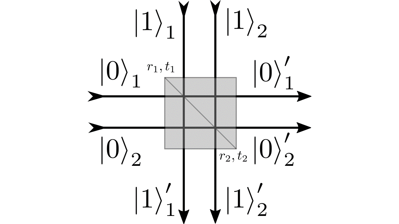 Figure 1
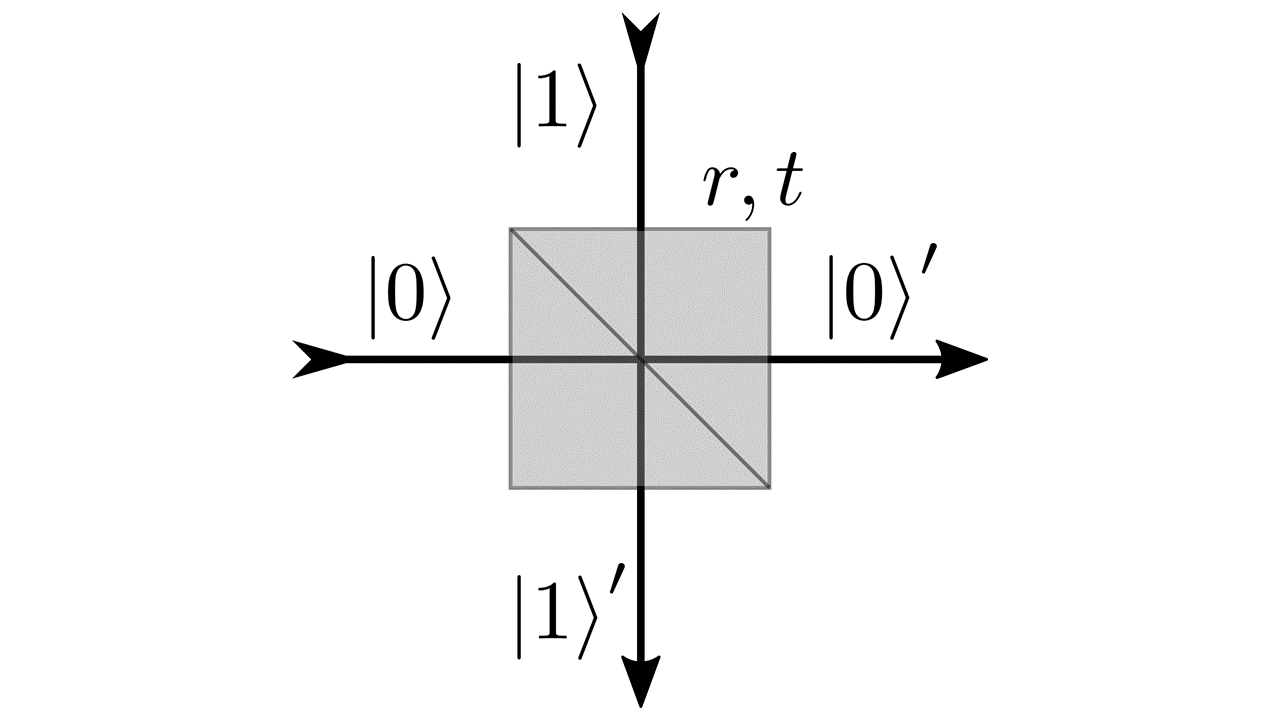 Figure 2
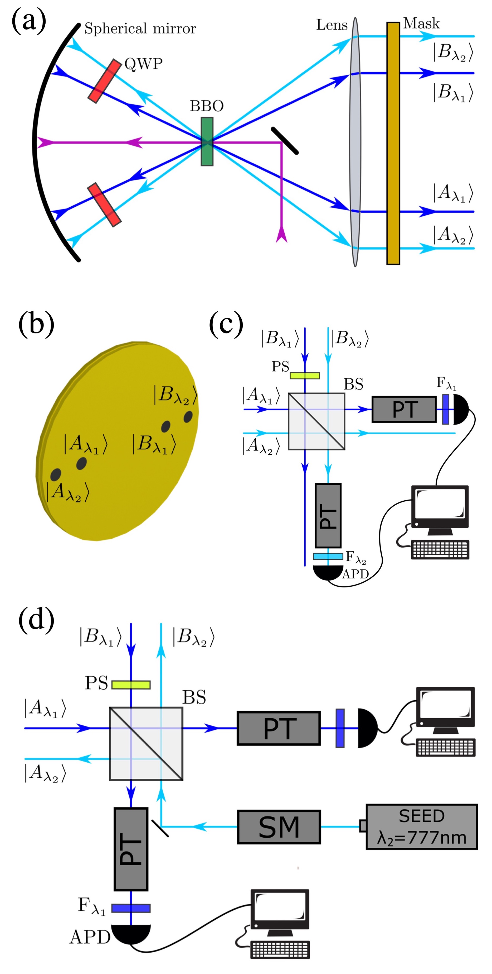 Figure 1
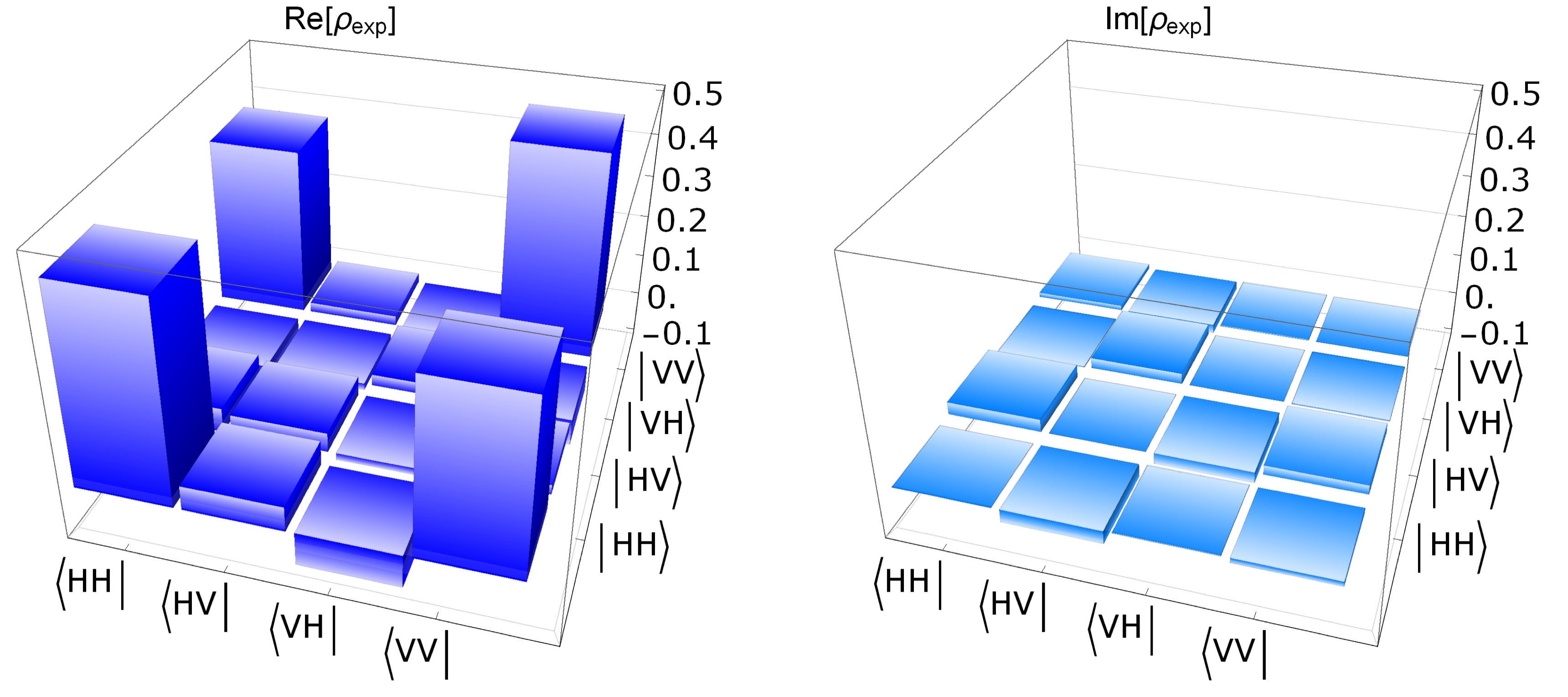 Figure 2
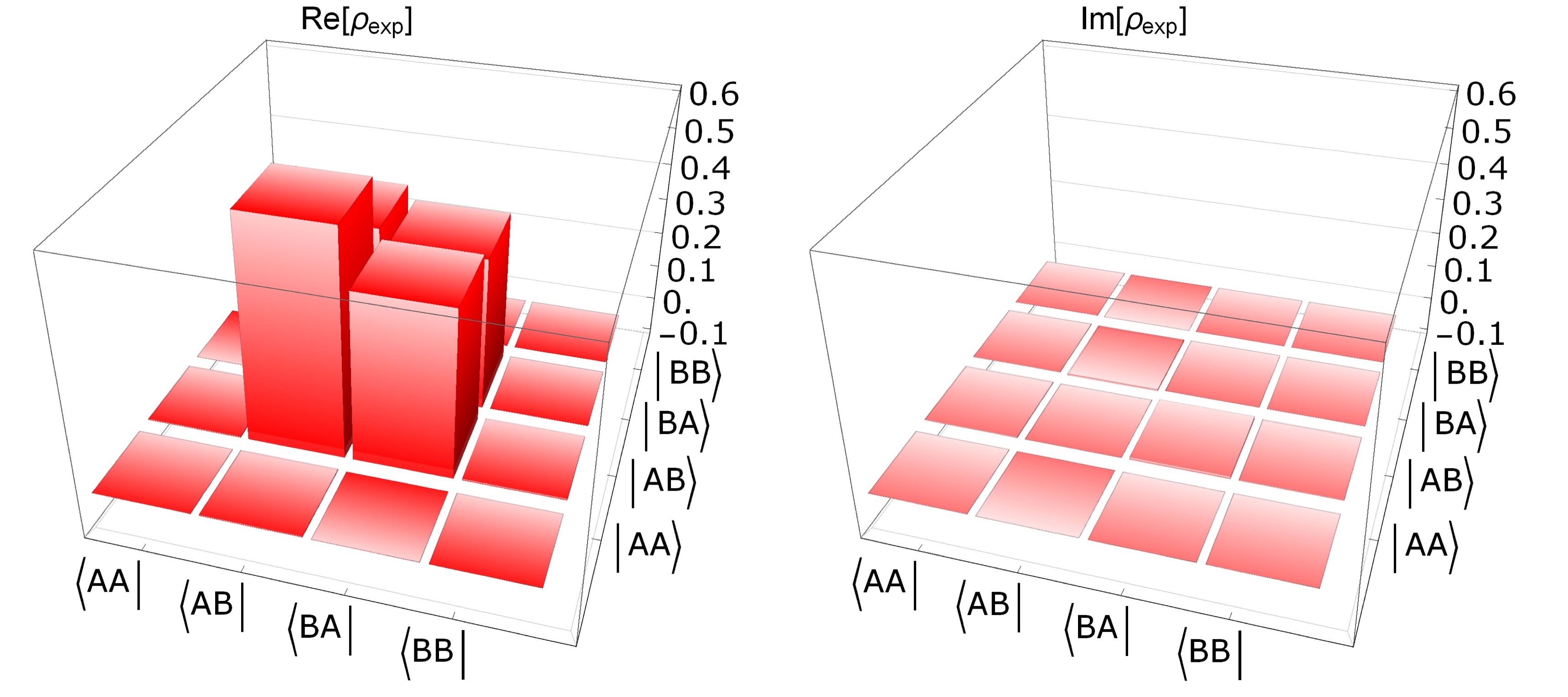 Figure 3
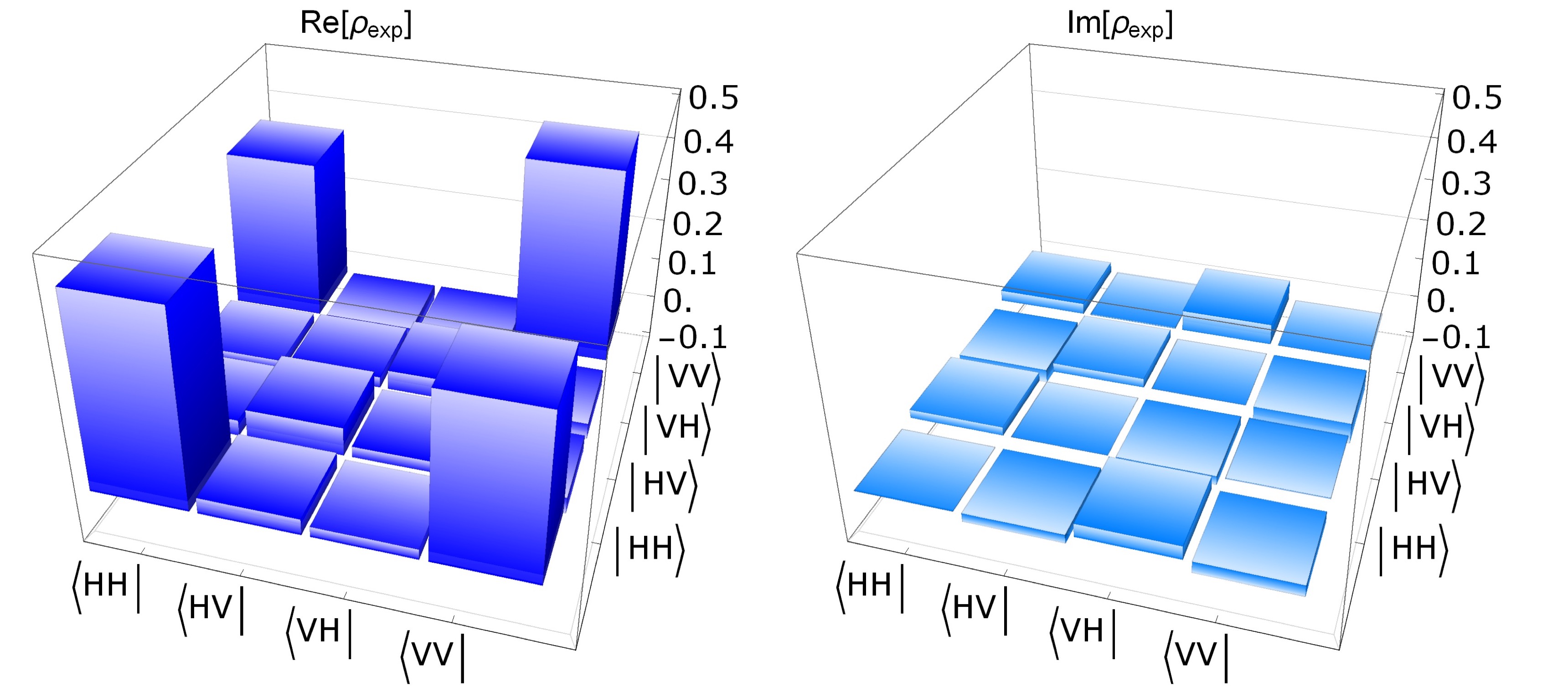 Figure 4
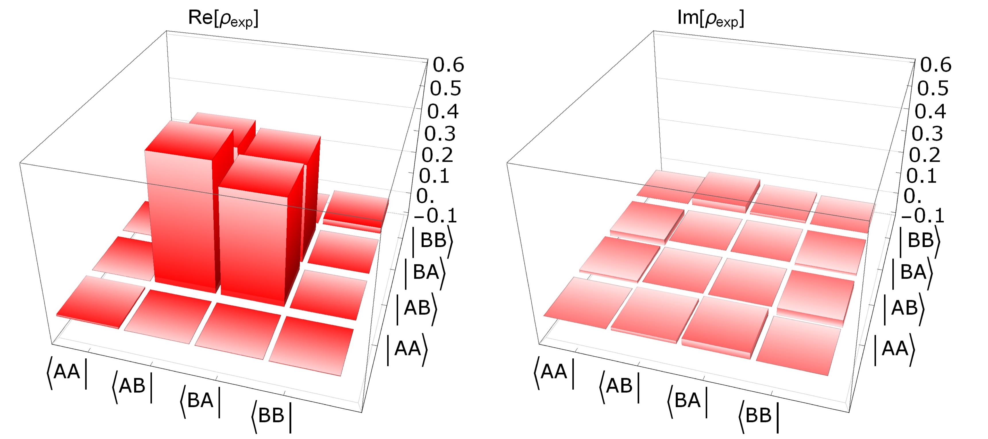 Figure 5
| Parameter | Path QST | Polarization QST | Path SET | Polarization SET |
|---|---|---|---|---|
| F | 0.9430.002 | 0.8570.008 | 0.9340.001 | 0.8140.008 |
| Tr() | 0.9090.003 | 0.7720.014 | 0.8860.001 | 0.6940.012 |
| 0.7850.005 | 0.5770.026 | 0.7790.001 | 0.4110.022 | |
| 0.8860.003 | 0.7590.017 | 0.8830.001 | 0.6410.017 |
| Parameter | nm | nm |
|---|---|---|
Peer Reviews
No public reviews on file for this paper yet. If you reviewed it on a platform where reviews are public (OpenReview, ICLR, NeurIPS, ICML), you can paste yours below so the community can read it here.
Videos
No videos yet. Explain this paper in a talk, walkthrough, or lecture? Add one.
Stimulated Emission Tomography: Beyond Polarization
Mario Arnolfo Ciampini, Andrea Geraldi,Valeria Cimini
Dipartimento di Fisica, Sapienza University of Rome, Piazzale Aldo Moro 5, 00185 Rome, Italy
Chiara Macchiavello
Dipartimento di Fisica, University of Pavia, via Bassi 6, 27100 Pavia, Italy
INFN Sezione di Pavia, via Bassi 6, I-27100, Pavia, Italy
CNR-INO, largo E. Fermi 6, I-50125, Firenze, Italy
J.E. Sipe
Department of Physics, University of Toronto, 60 St. George St., Toronto, ON, M5S 1A7, Canada
M. Liscidini
Dipartimento di Fisica, Università degli studi di Pavia, Via Bassi 6, 27100 Pavia, Italy
Paolo Mataloni
Dipartimento di Fisica, Sapienza University of Roma, Piazzale Aldo Moro 5, 00185 Rome, Italy
Abstract
In this work we demonstrate the use of stimulated emission tomography to characterize a hyper-entangled state generated by spontaneous parametric down-conversion in a CW-pumped source. In particular, we consider the generation of hyper-entangled states consisting of photon pairs entangled in polarisation and path. These results extend the capability of stimulated emission tomography beyond the polarisation degree of freedom, and demonstrate the use of this technique to study states in higher dimension Hilbert spaces.
Quantum state tomography (QST) is the task of experimentally identifying the density matrix describing a quantum state Altepeter et al. (2005a). For quantum optical systems, it involves a number of coincidence measurements, depending on the size of the Hilbert space under investigation. For instance, for two polarization-entangled photons, -1=15 independent polarization-resolved coincidence measurements are required Altepeter et al. (2005a). More generally, the dimension of the Hilbert space, and thus the number of measurements required, depends on both the number of photons and the degrees of freedom (DOFs) - such as polarization, spatial structure, etc. – that are involved.
While in the initial work on QST of photonic states only one DOF at a time - typically polarization White et al. (1999) - was considered, in the last fifteen years there has been growing interest in exploiting quantum correlations using different photon DOFs simultaneously. In particular, even states that are entangled in every DOF have been demonstrated by Kwiat et al. Barreiro et al. (2005), where the state of one photon pair belongs to a 36-dimensional Hilbert space. The generation and manipulation of such states is of paramount importance in quantum optics, for it allows for an increase in the information that can be stored in a state without the need for an increased number of photons. Yet the QST of these states can be extremely challenging, with large numbers of difficult coincidence measurements required.
In the last few years, there has also been progress in the generation and manipulation of non-classical light by exploiting parametric fluorescence in photonic integrated circuits (PICs), using either spontaneous parametric down conversion (SPDC) or spontaneous four-wave mixing (SFWM) Boitier et al. (2014); Horn et al. (2012); Grassani et al. (2015); Silverstone et al. (2015); Chen et al. (2016). In these systems, light confinement at the micron scale leads to an enhancement of the efficiency of parametric fluorescence over what can be achieved with bulk crystals by up to seven orders of magnitude Atzeni et al. (2018). In the case of PICs the use of the polarization DOF is particularly challenging, and so path and energy are usually the preferred DOFs for quantum correlations. Even here QST is difficult, for the photon collection efficiency is still done off-chip and is plagued by coupling and propagation losses, as well as less-than-ideal detector efficiencies.
A few years ago, it was suggested that sources based on parametric fluorescence could also be characterized by Stimulated Emission Tomography (SET), which relies on the relation between the spontaneous and stimulated emission of photon pairs Liscidini and Sipe (2013). In SET the density matrix that would be relevant in a spontaneous process is determined by characterizing the associated stimulated process. Thus higher signal-to-noise can be achieved than in a spontaneous emission experiment, and the equipment necessary for coincidence measurements (i.e. single-photon detector) is usually not required. The validity of this approach has been demonstrated for polarization-entangled photon pairs generated by a sandwich BBO crystal source Rozema et al. (2015), with the dependence of the polarization density matrix on the energies of the emitted photons generated reported in Fang et al. (2016) for SFWM in optical fibers. However, so far, only polarization density matrices have been reconstructed via SET experiments. Demonstrating SET on other DOFs than polarization would be an important milestone towards the use of this powerful tool for the characterization of sources of non-classical light in several platforms.
In this work we demonstrate SET on multiple DOFs for the first time, and determine the reduced density matrix for both polarization and path in the case of a two-photon hyperentagled state. These results are particularly important, not only because the path Hilbert space can have, in principle, infinite dimension, but also because we extend the use of SET to one of the preferred DOFs in PICs Crespi et al. (2011); Corrielli et al. (2014); Silverstone et al. (2013); Wang et al. (2018). Indeed, previous characterizations of photon pair sources via stimulated emission have shown that in integrated devices or optical fibers, where there is a discrete set of spatial modes, SET can outperform traditional methods based on parametric fluorescence in terms of resolution and speed Eckstein et al. (2014); Fang et al. (2014); Jizan et al. (2015); Grassani et al. (2016); Fang et al. (2016). However, here we make a different choice and use SET to study the generation of photon pairs in a bulk nonlinear crystal, in which the realization of entanglement in multiple DOFs is easier. More importantly, we want to compare SET results with those obtained with QST, allowing for their better understanding.
We consider a mm long type I crystal of -Barium Borate (BBO), excited in two opposite directions by a 100 mW, vertical polarized (V), continuous-wave (cw) pump laser with wavelength nm (GENESIS, Coherent) (see Fig. 3). In the first passage through the BBO crystal, pairs of horizontally polarized (H) photons could be emitted and would pass through a wide-band quarter wave plate (QWP), be back-reflected by a spherical mirror, and pass again through the same QWP to be vertically polarized. The mirror, with radius of curvature cm, is placed a distance from the BBO crystal. The pump laser is also back-reflected by the same mirror and excites the BBO crystal a second time, with the possibility of creating a pair of horizontally polarized photons. When spatial and temporal overlapping of the two generations is guaranteed by a proper arrangement of the optical elements and the cw pump, respectively, the generated photons are in a quantum superposition. This source is a modified version of that reported earlier Barbieri et al. (2005), in which path-polarization hyperentangled states are generated in an energy-degenerate configuration. However, in the present implementation the photons are generated at two different wavelengths: nm and nm. Since photon pairs are emitted in a spatial conical distribution determined by the SPDC phase-matching condition, path entanglement is expected and can be verified by selecting photons along four directions by using a four-hole mask having the holes located along the horizontal diameter of the circular section of the emission cone (see Fig. LABEL:fig:mask).
In this simple picture, polarization and path DOFs are independent. Thus one would expect the hyperentangled state
[TABLE]
with polarization state
[TABLE]
and path state
[TABLE]
where photons are labeled by their wavelength and can exit either through the left (A) or the right (B) hole with respect to the center of the mask. Finally, and are phase factors, with the former depending on the displacement of the spherical mirror along the laser pump direction, and the latter being controlled by means of a phase shifter (PS) consisting of a thin glass plate placed in one of the four spatial modes.
First, we characterize the generated state via QST for both DOFs by measuring the mean values of the corresponding Pauli operators , and . As usual, in the case of polarization, this is done by means of QWPs, half wave plates (HWPs), and polarizing beam splitters (PBS); a PS and a beam splitter (BS) are used to construct the necessary observables in the path DOF (see Fig. LABEL:fig:QST). Finally, single-mode fibers are used to direct photons to two single-photon avalanche photodetectors (APDs), while two nm-bandwidth interference filters () are used to separate the photons according to their wavelength and . The measured coincidence rate is about Hz in a gate temporal window of ns with a coincidence to accident ratio of the order of 100. QST required about 10 minutes. The path and polarization density matrices reconstructed using these experimental data by hypercomplete quantum state tomography Altepeter et al. (2005a); James et al. (2001) are shown in Fig. 2 and Fig. 3, respectively. From the density matrices, we also calculate fidelities, purities, tangles, and concurrences (see Tab. 1.) Uncertainties are computed by assuming the coincidence counts to be Poissonian distributed, and neglecting any systematic error.
The path fidelity is close to unity, with a small discrepancy that we attribute to the limited visibility of the interferometer used in the QST measurement. In contrast, the polarization fidelity is considerably lower than unity, which indicates that our initial model of the source may be too simplistic. This is confirmed by the purity values reported in Tab. 1, where the polarization purity is significantly less than that of the path.
The difference in purity between path and polarization suggests that one might have to consider additional DOFs for a correct interpretation of the results. In our initial description, we did not take into account that the photons are collected within a certain momentum range associated with the finite aperture of the hole in the mask. Taking this into account requires the introduction of additional DOF and its corresponding Hilbert space, such that:
[TABLE]
where is associated with the momentum DOF determined by the hole size. Thus, the generated state becomes:
[TABLE]
where
[TABLE]
since polarization and momentum are entangled. This would explain the unit purity for the path density operator and a lower purity for the polarization density operator. This description is consistent with previous experimental results Rozema et al. (2015); Fang et al. (2016); Altepeter et al. (2005b).
We now turn to the SET measurements, remembering that in our experiment the two generated photons have different energies. This choice is motivated by our use of a cw-pumped source, which results in a lower efficiency than that of sources studied in earlier works Rozema et al. (2015); Fang et al. (2016). In our scenario, the use of a seed with the same wavelength as that of the generated light would lead to a generated signal intensity comparable with that of the seed light scattered by the nonlinear crystal. Thus, to improve the signal-to-noise ratio, it is convenient to work with non-degenerate SPDC, where the seed beam can be filtered before detection.
In order to determine the density matrix by SET, we need to construct a proper seed beam that stimulates the pair generation. Given the particular geometry of our source, this can be done by removing the detector of the photon and placing a cw laser operating at this wavelength, which inputs light in the very same single-mode fiber used to collect the photons in the spontaneous process (see Fig. ). Parametric amplification at wavelength is demonstrated by the enhancement of the photon generation rate by four orders of magnitude, with a count rate of almost MHz. A QWP, a HWP, a PS, and a BS are used to adjust the input parameters of the seed laser, as required by the SET protocol Liscidini and Sipe (2013). The measurement time for the SET took 2-3 minutes in total. In particular, we modify the seed characteristics such that the light exiting the setup mimics the properties (polarization and path) of the photon that would be detected in the corresponding QST measurements for SPDC. This allows us to directly estimate the average number of pairs that would be detected in QST and calculate the corresponding density matrices.They are reported in Fig. 4 and Fig. 5 for polarization and path DOFs, respectively. Finally, fidelities, purities, tangles, and concurrences are shown in Tab. 1.
The similarity between the density matrices obtained with SET and QST is such that a reader might be tempted to compare the results directly. Yet this should be done with care, for in general energy and momentum correlations with other DOFs are weighted differently in these two characterization approachesRozema et al. (2015). In SET, pair emission is stimulated using a cw laser, with the pairs being emitted and analyzed in a very narrow frequency range (in our case the seed laser had a linewidth shorter than nm). On the contrary, the smaller generation rates in QST typically require the collection of the emitted pairs over much larger energy and momentum ranges. When this is properly taken into account, for example by performing energy-resolved SET measurements and averaging on the results, one finds complete agreement between the techniques Fang et al. (2016).
From these considerations, in our experiment one expects some differences between SET and QST results for polarization, as we know from the QST characterization that correlations with other DOFs are present (see Eq. (6)). Therefore, although at first glance the density matrices of Fig. LABEL:fig:QST and LABEL:fig:SET are very similar, it is not surprising that the purities, tangles, and concurrences obtained by SET differ from the values obtained using QST by 10% to 25%. The situation for the path DOF should be rather different, as from Eq. (5) we do not expect significant correlations with other DOFs. And indeed, there is a high path purity shown with all the corresponding parameters for SET and QST in very good agreement, showing negligible discrepancies for tangle and concurrence, and differences of only 1-2% for fidelity and purity. Such small differences may be attributed to systematic errors, which are not included in the uncertainties shown in Tab. 1. For example, an ideal implementation of SET requires all the seeded light to exit the source in the same mode Liscidini and Sipe (2013), while we verified that this is not so in our experiment, since some seed light is scattered by the apertures in the mask and by other optical elements of our setup.
In conclusion, we have demonstrated that SET can be used to characterize quantum states that are entangled in more than one degree of freedom, moving beyond start-of-the-art experiments that have only considered the polarization degree of freedom. In particular, we have performed SET on a source generating photons hyperentangled in path and polarization, revealing all the main features of our complex system. The demonstration of SET on the path DOF is a significant advance on the road to the implementation of this powerful technique on many different sources, including integrated devices, where DOFS different than polarization are used in quantum information studies and protocols, and where the SET advantages of speed and resolution will be most useful.
I SUPPLEMENTAL:Purity and Hilbert spaces
In this section we give more details about the connection between the purity of reduced density matrices associated with path and polarization degrees of freedom (DOFs).
Since the measured purity of the reduced density operator characterizing the path degree of freedom is close to unity, it is reasonable to consider the full state of the system as essentially pure. Then the simplest assumption would be that one could consider the relevant Hilbert space to be a direct product of a Hilbert space associated with the path of the photons and one associated with their polarization,
[TABLE]
but this will not suffice. Indeed, a ket in this Hilbert space could always be Schmidt decomposed,
[TABLE]
with
[TABLE]
and we would have
[TABLE]
while experimentally the purity of the reduced density operators associated with path and polarization are significantly different.
Thus we consider the experimental scenario in more detail, and take into account the finite size of the holes in the mask. In the simple argument above, these holes were associated with the Hilbert space of the path of the photons. But in fact, photons with different momenta will be collected by the same hole, and the mask will then effectively lead to a ?trace? over those momenta, with part of information related to the emission direction lost once the photons are collected by the fiber. In particular, this information is related to small deviations from the propagation direction given by the center of the nonlinear crystal and that of the holes in the mask. For these reasons, we start with the generated state
[TABLE]
where is the biphoton wave function associated with the pair generated for a forward (reflected) pump, where , and is the idler photon state of momentum and polarization , etc.
The mask is described by the projector
[TABLE]
where corresponds to the positions on the mask, left (L) or right (R) with respect to the center of the holes for idler and signal (see Fig. 1 (a); or , for example), while indicates the 2-dimensional integration range over determined by the size of the holes in the mask, corresponds to the hole centers. This, leads to the state:
[TABLE]
Here the Hilbert space can be considered a direct product of Hilbert spaces associated with the paths, the polarization, and the distribution of momenta within each hole that identifies the paths,
[TABLE]
where is the polarization Hilbert space, the path Hilbert space, which depends on the hole position through and , and the Hilbert space associated with the momentum DOF determined by the hole size. This factorization is natural because one can define the operators such as , which describes the creation of an idler photon exiting in the path , having polarization , and with momentum in the direction given by . These operators satisfy the commutation relations
[TABLE]
Thus, we can rewrite
[TABLE]
where . Given the symmetry of our source and mask, we can safely assume that polarization and DOFs are independent of the path, and take
[TABLE]
which allows us to write
[TABLE]
with
[TABLE]
where the and states are denoted by and , and
[TABLE]
We notice that, while the purity of the reduced path density operator given by (24) is unity, in general the purity of the polarization reduced density operator is less than unity, because of the correlations between the polarization and the collection angle associated with the size of the holes in the mask.
II Visibility and Purity
In the following section we justify how the expected purity for a state encoded in the path degree of freedom can be lower than unity, if we accounted for imperfections of the experimental apparatus. We describe the link between the visibility of the interference of a pure quantum state entering a lossless unbalanced Beam Splitter (LUBS) and the purity of a mixed state that enters in an lossless balanced Beam Splitter (LBBS) and generates the same visibility. In this way we can calculate the maximum expected value of the purity for a state entering a lossless unbalanced BS.
II.1 1 qubit
II.1.1 Visibility with a pure state and unbalanced beam splitter
Suppose we have a qubit encoded in path degree of freedom and that the state of the qubit is represented by the normalized ket
[TABLE]
where and are the eigenstates of the path and the input arms of a LUBS (see Fig.6).
The LUBS is characterized by a transmittivity coefficient and a reflectivity coefficient (), such that
[TABLE]
The LUBS acts on , as follow:
[TABLE]
where the kets and represent the output modes of the LUBS. The evolution of is:
[TABLE]
The probability of obtaining after a measurement, for instance, depends on the phase , and it is maximized (minimized), when (), such that:
[TABLE]
The visibility V of the interference in such case is:
[TABLE]
where we have used the relation (27) in the third passage. If , then . This result shows the dependence of the visibility to the parameters of the LUBS.
II.1.2 Purity of a mixed quantum state in a ideal beam splitter
We now consider a mixed state as input of an LBBS, namely:
[TABLE]
where is the 2 dimensional identity matrix and p is a parameter connected to the purity of the state. The state after an LBBS () becomes:
[TABLE]
We proceed as before, evaluating the probability of obtaining state after a measurement of the system, and then we calculate the visibility , such that:
[TABLE]
We can then substitute the value of in Eq. 32 and obtain
[TABLE]
From this, we recover the purity P of the state, as a function of :
[TABLE]
and
[TABLE]
II.1.3 Bounds on the purity of a state, given an experimental visibility
The previous results show that can have a state with if we have a LUBS. Indeed, combining 37 and 31, and assuming , we find that . We can say that if the state that is measured by our non-ideal setup is a mixed state with maximum purity given by Eq. (36).
II.2 2 qubits
Now we address the 2-qubit case. Suppose we have a path entangled state
[TABLE]
where the label 1 (2) represent the first (second) qubit. We consider the eigenstates as kets representing the input modes of two LUBSs (see Fig.7).
Each LUBS has its own values of and :
[TABLE]
where .
After the interaction with the LUBS we obtain
[TABLE]
If we look at one of the four elements of the state, for example at the ket , we can evaluate the maximum and minimum value of the interference
[TABLE]
and the visibility
[TABLE]
This show that one can obtain visibility different from unity even if the input state is pure state. For this reason we want to find a mixed state that gives the same visibility when interacting with LBBS and then find a link between the visibility and the purity of the mixed state.
In order to do that we write the state as
[TABLE]
In order to determine the value of p we apply the LBBS transformation to the state
[TABLE]
Now we impose that the visibility of interference of on the LBBS is equal to the one of the pure state on the LUBS. The maximum reached after the LBBS is the sum of the maximum of the interference due to the pure state contained in and the contribution of the mixed state of , while the minimum is given only by the mixed state because for the pure state the interference is complete. So
[TABLE]
We can then substitute the value of in Eq. (43) and obtain
[TABLE]
Now we can calculate the square of the density matrix
[TABLE]
and the purity
[TABLE]
So the link between the visibility given by a pure state entering an unbalanced LUBS and the purity of a mixed state that enters an LBBS and that gives the same visibility is given by the Eq. (48). In this sense we can say that if the state that is measured by our imperfect setup is a mixed state with maximum purity given by Eq. (48).
We can then evaluate the maximum purity that can be reached with the BS used in our experiment. In our case the subscript of and denotes the different wavelengths of the photons. The numerical values of the BS’s parameters are listed in Table 2.
We obtain, through the Eq.(48), the maximum purity for horizontally and vertically polarized photons
[TABLE]
The values of the purity measured experimentally are
[TABLE]
The experimental data are compatible with these theoretical predictions, which are upper bounds for the purity.
III Measurement time
As mentioned in the manuscript, to the best of our knowledge, SET in a DOF other than polarization has never been attempted before. Thus we decided to use a source that could be characterized via traditional QST. As in the case of Ref.11, in which SET has been performed on a bulk crystal, here there is not significant advantage in terms of the time measurement, nor resolution. However, this choice gave the reader the opportunity to compare the results of SET and QST. The measurement time for the SET in both DOFs, polarization and path, took 2-3 minutes in total, while QST required about 10 minutes.
The reference list from the paper itself. Each links out to its DOI / PubMed record.
- 1Altepeter et al. (2005 a) J. B. Altepeter, E. R. Jeffrey, and P. G. Kwiat, Advances in Atomic, Molecular, and Optical Physics 52 (2005 a).
- 2White et al. (1999) A. G. White, D. F. V. James, P. H. Eberhard, and P. G. Kwiat, Phys. Rev. Lett. 83 , 3103 (1999) . · doi ↗
- 3Barreiro et al. (2005) J. T. Barreiro, N. K. Langford, N. A. Peters, and P. G. Kwiat, Phys. Rev. Lett. 95 , 260501 (2005) . · doi ↗
- 4Boitier et al. (2014) F. Boitier, A. Orieux, C. Autebert, A. Lemaître, E. Galopin, C. Manquest, C. Sirtori, I. Favero, G. Leo, and S. Ducci, Phys. Rev. Lett. 112 , 183901 (2014) . · doi ↗
- 5Horn et al. (2012) R. Horn, P. Abolghasem, B. J. Bijlani, D. Kang, A. S. Helmy, and G. Weihs, Phys. Rev. Lett. 108 , 153605 (2012) . · doi ↗
- 6Grassani et al. (2015) D. Grassani, S. Azzini, M. Liscidini, M. Galli, M. J. Strain, M. Sorel, J. E. Sipe, and D. Bajoni, Optica 2 , 88 (2015) . · doi ↗
- 7Silverstone et al. (2015) J. W. Silverstone, R. Santagati, D. Bonneau, M. J. Strain, M. Sorel, J. L. O’Brien, and M. G. Thompson, Nature Communications 6 , 7948 EP (2015) . · doi ↗
- 8Chen et al. (2016) Y. Chen, J. Zhang, M. Zopf, K. Jung, Y. Zhang, R. Keil, F. Ding, and O. G. Schmidt, Nature Communications 7 , 10387 EP (2016) . · doi ↗