GARCH density and functional forecasts
Karim M. Abadir, Alessandra Luati, Paolo Paruolo

TL;DR
This paper derives an explicit analytic form for the $h$-step ahead prediction density of a GARCH(1,1) process with Gaussian innovations, enabling exact risk measure calculations and analysis of non-Gaussianity in financial returns.
Contribution
It provides the first explicit formula for the GARCH prediction density and demonstrates its applications in risk measurement and distribution analysis, surpassing Monte Carlo methods.
Findings
Deviations from Gaussian distribution are sometimes significant.
Exact tail probabilities improve risk assessment accuracy.
Uncertainty regions reflect in-sample estimation uncertainty.
Abstract
This paper derives the analytic form of the -step ahead prediction density of a GARCH(1,1) process under Gaussian innovations, with a possibly asymmetric news impact curve. The contributions of the paper consists both in the derivation of the analytic form of the density, and in its application to a number of econometric problems. A first application of the explicit formulae is to characterize the degree of non-Gaussianity of the prediction distribution; for some values encountered in applications, deviations of the prediction distribution from the Gaussian are found to be small, and sometimes not. the Gaussian density as an approximation of the true prediction density. A second application of the formulae is to compute exact tail probabilities and functionals, such as the Value at Risk and the Expected Shortfall, that measure risk when the underlying asset return is generated by a…
Click any figure to enlarge with its caption.
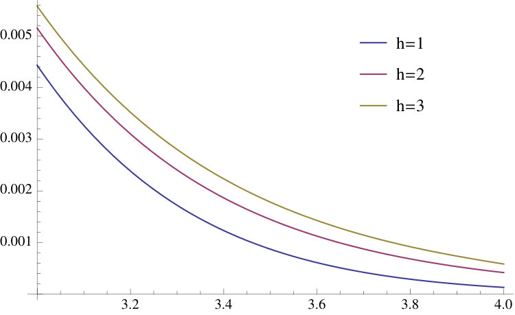 Figure 1
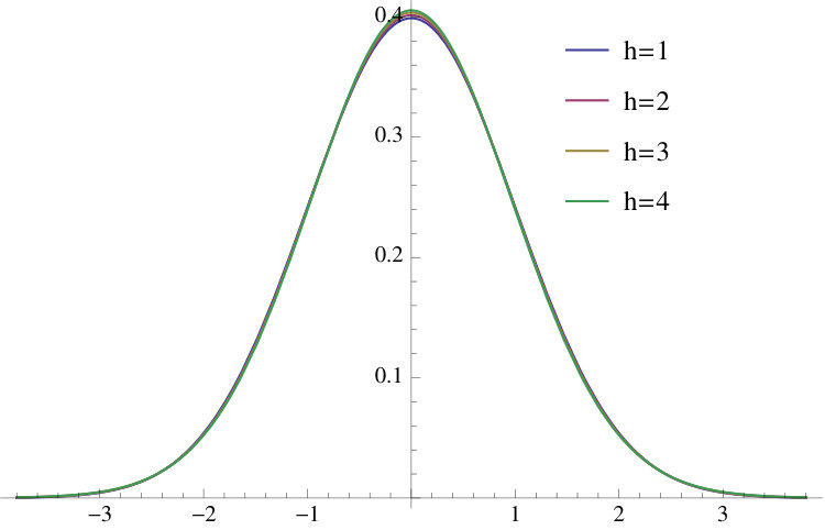 Figure 2
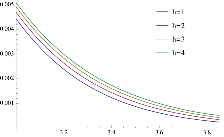 Figure 3
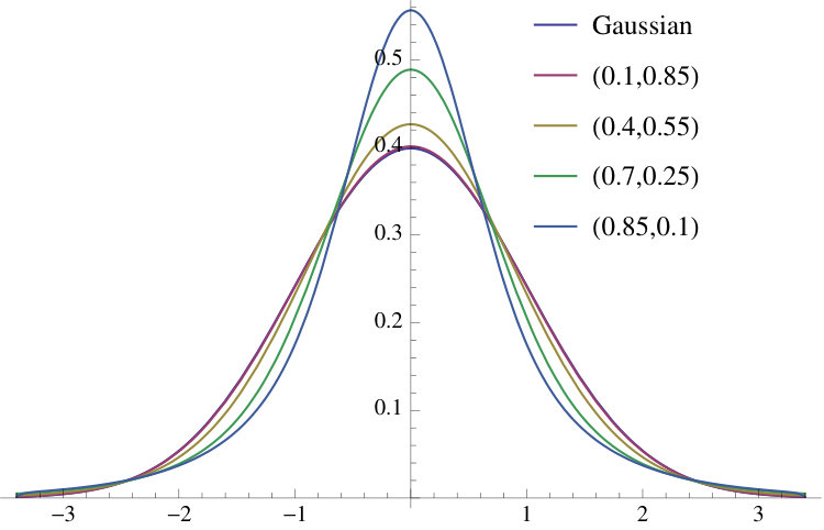 Figure 4
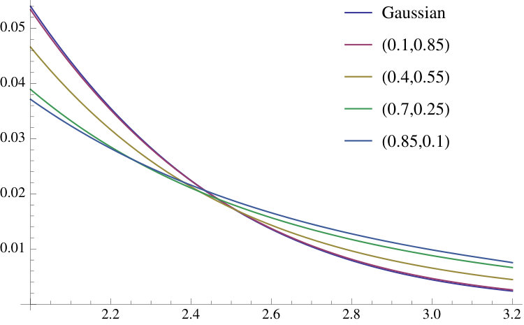 Figure 5
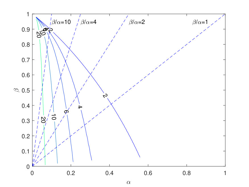 Figure 6
| exact | # of iterations | Gaussian | ratio=Gaussian/exact | |
|---|---|---|---|---|
| 0.05 | 3 | 1.0020 | ||
| 0.025 | 3 | 0.9982 | ||
| 0.01 | 3 | 0.9924 | ||
| 0.005 | 4 | 0.9872 |
| exact | Gaussian | ratio=Gaussian/exact | |
|---|---|---|---|
| 0.05 | 2.0745 | 2.0627 | 0.9943 |
| 0.025 | 2.3620 | 2.3378 | 0.9898 |
| 0.01 | 2.7121 | 2.6652 | 0.9827 |
| 0.005 | 2.9612 | 2.8919 | 0.9766 |
| 0.025 | 0.01 | 0.005 | ||
|---|---|---|---|---|
| 7.0710E+11 | 1.1604E+12 | 2.3680E+12 | 4.2104E+12 | |
| 1.2213E+12 | 2.0043E+12 | 4.0900E+12 | 7.2722E+12 |
| 0.025 | 0.01 | 0.005 | ||
|---|---|---|---|---|
| 5.0484E+12 | 1.2813E+13 | 4.0575E+13 | 9.3989E+13 | |
| 8.7196E+12 | 2.2131E+13 | 7.0081E+13 | 1.6234E+14 |
| interval for | interval for | number of extremes | ||||||
|---|---|---|---|---|---|---|---|---|
| min | max | min | max | derived from surface points | ||||
| Microsoft stock returns | 2.6733 | 2.6957 | 4 out of 4 | |||||
| One simulation run | 2.6652 | 2.9144 | 2 out of 4 | |||||
Peer Reviews
No public reviews on file for this paper yet. If you reviewed it on a platform where reviews are public (OpenReview, ICLR, NeurIPS, ICML), you can paste yours below so the community can read it here.
Videos
No videos yet. Explain this paper in a talk, walkthrough, or lecture? Add one.
Taxonomy
TopicsMarket Dynamics and Volatility · Monetary Policy and Economic Impact · Financial Risk and Volatility Modeling
GARCH density and functional forecasts111Information and views set out in this paper are those of the authors and do not necessarily reflect the ones of the institutions of affiliation.
The authors acknowledge useful comments from Enrique Sentana, Robert Engle, Eric Renault, Leopoldo Catania, Barbara Rossi, Dimitris Politis, Ngai Chan, Christian Brownlees, Nour Meddahi, Torben Andersen, two anonymous referees, as well as from participants to seminars in University of Verona and Bocconi University of Milan, the Seventh Italian Congress of Econometrics and Empirical Economics 2017, EC2 2017 in Amsterdam, Barcellona GSE Summer Forum 2017 and the NBER-NSF Time Series Conference 2018.
Karim M. Abadir222Email: [email protected], ORCID: 0000-0001-5637-9513.
Alessandra Luati333Email: [email protected], ORCID: 0000-0001-6407-9385.
Paolo Paruolo444Email: [email protected], ORCID: 0000-0002-3982-4889,
Corresponding author.
Address: European Commission, Joint Research Centre (JRC), Via Enrico Fermi 2749,
TP 723, 21027 Ispra (VA), Italy
Business School, Imperial College London, UK
Department of Statistical Sciences “Paolo Fortunati”, University of Bologna, Italy
European Commission, Joint Research Centre (JRC), Ispra (VA), Italy
Abstract
This paper derives the analytic form of the -step ahead prediction density of a GARCH(1,1) process under Gaussian innovations, with a possibly asymmetric news impact curve. The contributions of the paper consists both in the derivation of the analytic form of the density, and in its application to a number of econometric problems. A first application of the explicit formulae is to characterize the degree of non-Gaussianity of the prediction distribution; for some values encountered in applications, deviations of the prediction distribution from the Gaussian are found to be small, and sometimes not. the Gaussian density as an approximation of the true prediction density. A second application of the formulae is to compute exact tail probabilities and functionals, such as the Value at Risk and the Expected Shortfall, that measure risk when the underlying asset return is generated by a Gaussian GARCH(1,1). This improves on existing methods based on Monte Carlo simulations and (non-parametric) estimation techniques, because the present exact formulae are free of Monte Carlo estimation uncertainty. A third application is the definition of uncertainty regions for functionals of the prediction distribution that reflect in-sample estimation uncertainty. These applications are illustrated on selected empirical examples.
keywords:
GARCH(1,1), Prediction density, Functionals, Value at Risk, Expected Shortfall
JEL:
C22 , C53 , C58 , G17 , D81
Contents
1 Introduction
Since their introduction in Engle (1982) and Bollerslev (1986), Generalised AutoRegressive Conditional Heteroskedasticity (GARCH) processes have been widely employed in financial econometrics, see e.g. Bollerslev et al. (2010). In the GARCH original formulation, the conditional distribution of innovations was typically assumed to be Gaussian; even with Gaussian innovations, GARCH processes were shown to generate volatility clustering and, when stationary, an unconditional distribution with fatter tails than the Gaussian, see e.g. Bollerslev et al. (1992).
GARCH processes can include several lags of the past squared shocks and several lags of the past volatility; in practice, however, the GARCH(1,1) model with is often found to offer a good fit for asset returns, and it is usually preferred to GARCH models with more parameters, see Tsay (2010) section 3.5, or Andersen et al. (2006), section 3.6. Moreover, many multivariate GARCH models are built on the univariate GARCH(1,1), see e.g. Engle et al. (2019) and references therein. In this sense the GARCH(1,1) is both the prototype and the workhorse of GARCH processes in practice.
GARCH processes map news into the conditional volatility; the function obtained by replacing past conditional volatilities with unconditional ones was called by Engle and Ng (1993) the news-impact-curve. For GARCH(1,1) processes, this curve yields the same value of volatility for positive and negative shocks, i.e. it is symmetric. Glosten et al. (1993) (henceforth GJR) extended the GARCH setup to allow for asymmetric news impact curve responses to negative shocks.
Many measures of risk are functions of the prediction distribution of asset returns. These measures include the Value at Risk, which is a quantile of the prediction distribution of the asset return, see Jorion (2006), as well as the Expected Shortfall, see Patton et al. (2019) and Arvanitis et al. (2019). The latter is the expected value of the prediction distribution of the asset return in the left tail of the prediction density below the Value at Risk; this measure has been recently re-emphasised by the Third Basel Accords. Both measures are functionals of the prediction distribution of asset returns.
The prediction distribution of a GARCH(1,1) hence plays an important role for the computation of risk measures in financial applications. This distribution is not known in analytic form beyond the distribution of innovations for the 1-step ahead case, which is given by assumption when building the process, see e.g. Andersen et al. (2006), page 811 and Baillie and Bollerslev (1992).
The present paper derives the analytical form of the -step-ahead prediction density of a Gaussian GARCH(1,1), , with , also allowing for GJR-GARCH(1,1) with asymmetric news-impact-curve. The first contribution of the paper is theoretic, and consists in the form of the p.d.f. and c.d.f. of the prediction distribution. The results are obtained by marginalizing the joint density of the prediction observations, using integration and special functions, for any prediction horizon .The formulae are valid for stationary as well as non-stationary GARCH(1,1) processes.
The 2-step-ahead prediction distribution is obtained without imposing constrains on the values of the and coefficients. For the -step-ahead prediction distribution with , a condition on is required to guarantee integrability, which depends on how the coefficients are related to the last observed value of the volatility . Unless the last observed value of volatility is relatively low, a sufficient condition for integrability is larger than . Another sufficient condition that is independent of the last observed value of volatility is larger than .
As suggested by one referee, one could wonder how frequently the conditions and are satisfied by empirical estimates in practice. While this is ultimately an empirical question that depends on the data at hand, one could consider the estimates in Bampinas et al. (2018), who fit GARCH(1,1) models to all stock returns in the S&P 1500 universe, from January 2008 to December 2011, with daily observations. Their Table 1 reports a mean value of of (median ) with standard deviation of . If the empirical distribution of these estimates were Gaussian, the predicted frequency of estimates below (respectively ) would be 6.2% (respectively 1.1%). Typical values for estimates reported in textbooks and in empirical finance literature are also above . On this basis, one would expect or not to be binding restrictions in most practical applications.555Table 1 in Bampinas et al. (2018) reports a skewness of and kurtosis of , which indicate that the distribution is far from normal; unfortunately, no min or max values are reported in the table. Typical values in textbooks and in empirical finance literature can be found in Linton (2019) Table 11.4, Tsay (2010) page 136, Francq and Zakoian (2010) page 262, Engle et al. (2008) page 694; they are all greater than for daily, weekly and monthly returns.
The assumption of Gaussianity of the innovations is central in the derivations in the paper, which employs analytical integration and special functions that are specific for this distribution. The approach in the derivation of the prediction distribution is expected to be amenable to extensions to non-Gaussian symmetric distributions of innovations. These extensions are not trivial and are not considered in the present paper.
A first application of the present results is the characterization of the degree of non-Gaussianity of the prediction distribution. This problem is relevant in practice, because the Gaussian density is often used as an approximation of the true prediction density, see e.g. Lau and McSharry (2010), page 1322. The exact formuale in this paper demonstrate that the prediction density can be very far from normal. However, for some parameter values encountered in applications, the discrepancy of the prediction density from the Gaussian density can be small, and this fact would support to the Gaussian approximation. Note that it is the analytic form of the prediction density derived in this paper that allows to measure this discrepancy.
A different question in this first area of application is the association of the coefficients of the GARCH with both the shape of the prediction distribution and the shape of the stationary distribution, when this exists. Under stationarity, the predictive distribution converges to the stationary distribution as the number of steps increases. The tail behavior of the stationary distribution of the Gaussian GARCH(1,1) has been studied extensively, see Mikosch and Starica (2000) and Davis and Mikosch (2009). The tails of the stationary distribution of both the volatility and of the GARCH process are of Pareto type, say. These properties are based on results for random difference equations and renewal theory obtained in Kesten (1973) and Goldie (1991).
The prediction density is found to resemble a Gaussian density (with appropriate variance) for high values of , and far from it for low values of it. Similarly, large values of are found to be associated with higher values of , i.e. a Pareto stationary distribution with more moments (the Gaussian has all moments).
A second application of the explicit formulae in this paper is to compute exact tail probabilities and functionals, such as Expected Shortfall, that measure risk when the underlying asset return is generated by a Gaussian GARCH(1,1). This improves on existing methods based on approximations or Monte Carlo (MC) simulations combined with (non-parametric) estimation techniques.
The so-far unknown analytic form of the prediction density of a GARCH has led econometricians to look for alternative approximate solutions. Alexander et al. (2013) have resorted to approximations based on the first 4 moments of the prediction distribution; Baillie and Bollerslev (1992) use a Cornish-Fisher expansion and a Johnson SU distribution using the first 4 moments of the GARCH(1,1) to fit the distributions.
Alternative methods for estimating the prediction density and risk measures such as the Value at Risk and the Expected Shortfall rely on MC simulations of the underlying GARCH processes, see e.g. Delaigle et al. (2016). All these MC methods implicitly assume that the density and that the unknown functionals are finite.666Delaigle et al. (2016) proposed a non-parametric root- consistent estimator of the stationary distribution of the (log-)volatility process where is sample size.
In this domain, the present exact formulae are key to prove that the density and the unknown functionals are finite, which is pre-requisite for MC methods to work. It must be noted, however, that MC methods have an additional layer of uncertainty – associated with MC estimation – that the exact methods proposed in this paper bypass entirely. Specifically, MC estimation of prediction functionals results in confidence intervals with positive length and coverage probability ; their counterpart based on the exact results of this paper can be represented by confidence intervals with length equal to 0 and coverage probability 1. Hence the exact methods in this paper are qualitatively superior to those based on MC methods, in addition to being much more parsimonious in terms of required calculations.
A third application of the exact formulae in this paper is to provide uncertainty intervals for (functionals of) the prediction distribution that reflect in-sample estimation uncertainty. This allows one to map estimation uncertainty onto forecast uncertainty for the risk measures and to construct the associated forecast intervals that have a pre-specified (asymptotic) coverage level. For instance, one could predict the Expected Shortfall to lie in an interval with 95% confidence level, where the uncertainty reflects in-sample estimation uncertainty on the GARCH parameters. As already discussed for the second area of application, the exact methods in this paper lead to results that are structurally different from the ones based on MC methods. In fact the latter involve an additional layer of MC estimation uncertainty associated, which is avoided by the exact methods in the present paper.
The rest of the paper is organised as follows. Section 2 describes the general approach for the derivation of the prediction distribution. Section 3 states the main theoretical results. Section 4 discusses the degree of non-Gaussianity of the prediction distribution and compares the prediction distribution with the tails of the stationary distribution when this exists; this is the first area of application discussed above. Section 5 discusses the second area of application, i.e. how to apply the present exact results to the calculation of the Value at Risk and of the Expected Shortfall, and compares the obtained results with alternative estimators based on MC methods. Section 6 discusses the third area of application of the present analytical formulae to the construction of forecast intervals for risk measures that reflect in-sample estimation uncertainty. Section 7 concludes. Proofs are collected in the Appendix.
2 The prediction density
This section summarises the construction used to derive the prediction density as an integral, involving a product of densities of the innovations. Consider the asymmetric GJR-GARCH(1,1)
[TABLE]
where , and is the indicator function for the event , and is the sign of or ; these signs are the same because . The sequence is assumed to be i.i.d., centered around zero and with Gaussian p.d.f. .
Time is taken to be the starting time of the prediction, and it is assumed that one wishes to predict for some , conditional on the information set at time , which contains and ; the conditioning on and is not explicitly included in the notation of the prediction distribution for simplicity. 777The information set at containing contains and is consistent with observing from minus infinity to time 0 under stationarity. Note also that, because and are observed, also is observed.
Throughout the paper the values taken by the random variables , and are denoted and respectively, or sometimes and for simplicity, when this may not cause ambiguity.
The next Lemma reports consequences of the symmetry of the one-step-ahead density on relevant conditional p.d.f.s. In the Lemma, the following notation is used: , , where , denote values of and . The density of a random variable evaluated at is indicated as , and similarly indicates the conditional density for given , evaluated at and .
Lemma 2.1** (Densities).**
For symmetric , the p.d.f. is symmetric, i.e. , , and it is related to the p.d.f. of in the following way
[TABLE]
Moreover, and one has
[TABLE]
where depends on the value of z_{t-j}=x_{t-j}^{2}$$) and the sign of x_{t-j}$$) for via (2.1).
Next denote the set of all possible sign vectors by , . Densities are first computed conditionally on and later they are marginalized with respect to it. Here, conditioning on is relevant only for the GJR case .
The basic building block is given by the expression in (2.3). This density can be marginalised with respect to as follows
[TABLE]
Finally, can be marginalised with respect to the signs using the mutual independence of the signs and the fact that for all , due to the symmetry of . One hence finds
[TABLE]
where the sum is over , for . The prediction density is found by combining (2.5), (2.4), (2.3), (2.2).
The next Lemma reports a recursion for the volatility process, that turns out to be useful when solving the integral in (2.4). In the Lemma, the following notation is used: for , let and , where denotes a value of .
Lemma 2.2** (Volatility and transformations).**
The volatility process can also be written
[TABLE]
For , has the following recursive expression in terms of ’s
[TABLE]
with , which is measurable with respect to the information set at time [math]. Moreover, one has
[TABLE]
where \gamma_{h}:=\beta^{h-1}/(\prod_{t=1}^{h-1}{\color[rgb]{0,0,0}\definecolor[named]{pgfstrokecolor}{rgb}{0,0,0}\pgfsys@color@gray@stroke{0}\pgfsys@color@gray@fill{0}a}_{t}) and is the value of corresponding to .
3 Main results
The main results are summarised in Theorem 3.4 below. Before stating it, an auxiliary assumption is introduced. Define , and note that this is bounded by 0 and as and vary, . Moreover define the following function of : , which is used in the next Assumption.
Assumption 3.3**.**
- a.
For , let ;
- b.
For let .
It can be noted that , as . In Figure 1, the area above the curve represents the set for .
Note that depends on the ratio , where is the last known value in the information set. Relatively large values of correspond to , moderate values to and small values to . Note in fact, for instance, that corresponds to , an inequality one expects to be frequently valid. Note that , , , so that Assumption 3.3 requires (respectively when the last observed volatility is relatively large (respectively moderate) for the results in the paper for to hold. Only low values of the last observed volatility correspond to .
For , . Hence, unless the last observed volatility is very low i.e. , the sufficient condition (which could be possibly further analytically improved) requires .
In Theorem 3.4 below, is the confluent hypergeometric function of the second kind, also known as Tricomi function, see Abadir (1999) and Gradshteyn and Ryzhik (2007), section 9.21, whose integral representation is,
[TABLE]
with .
The function is used to define the following quantities:
[TABLE]
where , , . The multiple sum is defined for as , where the individual sums extend to if . For the sum and the product are empty and (3.2) reduces to .
Theorem 3.4** (GARCH(1,1) prediction density).**
Assume that are i.i.d. and let Assumption 3.3 hold; then one has, for , and
[TABLE]
where and is defined as where is defined in (3.2) and in Lemma 2.2. The expressions in (3.3) and (3.4) are absolutely summable for any finite or .
Proof.
See Appendix. ∎
Observe that the expression for does not depend on the points of evaluation or , and hence the coefficients can be computed only once for the whole densities. One can prove, see Lemma A.10 in the Appendix, that for . This implies that the terms converge to 0 for large in the product in (3.2).
Note also that for , equation (3.4) holds for any value of , while for it holds if and only if . For , the validity of the (3.4) is guaranteed by the sufficient condition , which is, however, not necessary.
The line of proof of Theorem 3.4 is the following: for the integral is solved by substitution and by using equation (3.1). For , subsequent (negative) binomial expansions of expression (2.7) for are required, whose validity is ensured by the inequality
[TABLE]
which is satisfied under Assumption 3.3, see Lemma A.11 in the Appendix.
Immediate consequences of Theorem 3.4 are collected in the following corollary.
Corollary 3.5** (C.d.f. and moments).**
The prediction c.d.f.s of and are given by the following expressions for , and
[TABLE]
with [math] odd moments for and even moments
[TABLE]
*where and depend on , see their definitions in Lemma 2.2 and in (3.2).
Note that in the moments calculations are made of finite sums extending to , involving the Tricomi functions, which do not fall in the logarithmic case as in Theorem 3.4; see Abadir (1999) for the logarithmic case. In fact, implies that
[TABLE]
is a finite sum, see Abadir (1999), which is proportional to the generalized Laguerre polynomial , where see e.g. Abramowitz and Stegun (1964) Chapter 22. For the moments of a GARCH(1,1), one can compare (3.6) with equations (34) and (35) in Baillie and Bollerslev (1992).
Some standardized densities of and the corresponding right tails are plotted in Figure 2 for . The curve is the standard Gaussian. Computations for Figures 2, 3 and 4 were performed in Mathematica.888When has mean 0 and standard deviation , the standardized variate is , with density .
Figure 3 shows the standardized prediction densities for and values of that range from to 8.5 () to 1/8.5 (). This figure shows that the deviations from the Gaussian case of the prediction density can be substantial; the prediction densities are more similar to a Gaussian when is large. Figure 4 shows the tails for the GJR-GARCH(1,1) case.
The formulae in Theorems 3.4 and Corollary 3.5 are alternating in sign. While (absolutely) convergent, the associated series was found in practice to be ill-behaved numerically when is very large, causing the oscillations in the terms of the series to become large before decreasing in amplitude toward zero, where ‘large’ refers to the greatest floating point number handled by the computer. Note that this is can be linked to large and/or small . This extreme behaviour implies accumulation of numerical errors, which can lead to inaccurate calculations of the prediction density.
Example 3.6* (Numerical accuracy).*
One such case can be obtained for the density of in formula (3.4), , in the following way: select for , and choose . This results in for the standardized p.d.f. of with . In this case, the oscillations of the terms in the series increase up to around the term of the series, before oscillations decrease toward zero; the resulting series truncated after its first 100 terms gave the negative number . Calculations performed in MATLAB 2018a on an Intel i7 Windows 10 computer. As a comparison, the same script applied to gave
In order to address these numerical accuracy problems when is large, the following theorem presents a different set of formulae for the prediction density. This alternative set has the advantage to allow computations in the far tails of the density, at the price of a slightly higher implementation cost.
Theorem 3.7** (Alternative formulae for the GARCH(1,1) prediction density).**
Under the same assumptions of Theorem 3.4 one has for , and
[TABLE]
For , is defined as , and
[TABLE]
*where denotes Pochhammer’s symbol, see Abadir (1999). *
For , where is a generalized Laguerre polynomial999 is the standard notation, see e.g. Abramowitz and Stegun (1964) Chapter 22., with the convention ; moreover where is defined as
[TABLE]
with , , . The expressions in (3.7), (3.8), (3.9), (3.10) are summable for any finite or .
The improved numerical performance of formula (3.8) is linked to the presence of the term when is large. In fact for the term , so that compensates the large terms of the type that appear in the sum for large . For , the term , so that does not influence the sum for small values of . Note, moreover, that all the terms in the series (3.7) and (3.8) are positive, so that there are no oscillations associated with different signs for the terms in the series.
Example 3.8* (Numerical accuracy - continued).*
In the same setup of Example 3.6, formula (3.8) is numerically accurate. In fact, all the terms in the series were found to be bounded by , with value of the density equal to , again using the first 100 terms of the series. Calculations were performed in the same environment as in Example 3.6. As a comparison, the same script applied to gave , which agrees with formula (3.4) in Example 3.6 up to the 5th digit (discrepancy equal to ).
The slightly higher implementation cost of formula (3.8) is associated with the presence of the generalised Laguerre polynomial in for . They are finite sums and add a moderate cost in terms of computations. Similar derivations to Corollary 3.5 can be performed on (3.7), (3.8) to derive the corresponding c.d.f.s.
4 Stationary distribution
The limit representation of the random variable in the stationary case can be found in Francq and Zakoian (2010) Theorem 2.1 page 24. The tail behaviour of the limit distribution is reviewed in Mikosch and Starica (2000) and Davis and Mikosch (2009). The tails of the stationary distribution of both the volatility and of the GARCH process are of Pareto type, say, where is a tail index. These properties are based on results for random difference equations and renewal theory obtained in Kesten (1973) and Goldie (1991).
The tail index of the stationary distribution depends on the coefficient and of the GARCH(1,1) process as well as on the one-step-ahead distribution. Examples of the tail index are given in Davis and Mikosch (2009); for Gaussian innovations, for , while for .
The index is the unique solution of . When is an integer, the expression simplifies to
[TABLE]
see Davis and Mikosch (2009) eq. (10). Substituting the moments from the distribution, and assigning values to over a grid of pre-specified values, one can solve (4.1) for , and hence for . This allows to compute (values of) the surface . Figure 5 reports the level curves of as a function of and obtained in this way. The figure also reports the lines where is constant. It is seen that, for large values of , and increase roughly together. This association is not present for small values of .
The relation between and fat-tailedness of the prediction density for finite horizon can be illustrated using the case . From Theorem 3.4,
[TABLE]
where and101010The quantity can be interpreted as the minimum value that can take, in the ideal case when (thus ) and is given, i.e. .
[TABLE]
Hence when one has with , see Abramowitz and Stegun (1964), eq. 13.1.8, so that all the Tricomi functions , for varying , tend to one.111111This is unlike in the case for fixed where the sequence of is decreasing to 0 for increasing . As a result, when the prediction distribution converges to a .
One concludes that both for the prediction density for and for the stationary distribution, the fat-tailedness of the distributions is small for large values of , unless is very close to 0.
5 Comparing exact formulae with simulation-based methods
This section describes the application of the formulae in the previous section to the calculation of the Value at Risk and of the Expected Shortfall, comparing them with alternatives based on Monte Carlo. This comparison is made under Gaussianity and Assumption 3.3, so that the formulae in the paper can be applied. The analysis in this and the remaining sections is for generic forecast horizon , while illustrations are made for and for simplicity and without loss of generality.
Let be some tail probability, such as 5%, and let be the Value at Risk, defined as the (negative) of the quantile of the prediction distribution, i.e. . Let also indicate the corresponding expected shortfall, i.e. , following standard notation, see e.g. Francq and Zakoian (2015).
Observe that may fail to exist when the underlying density has Cauchy tails. One implication of the exact results in Theorem 3.4 of Section 3 is that for finite the prediction of has thinner-than-Cauchy tails, and hence exists; this appears to be a central issue for the application of as a measure of risk.
The following subsections show first how the exact formulae can be applied in this context, and next their relative advantage over methods based on MC methods. The same advantages discussed for the quantification of the Value at Risk and the Expected Shortfall apply more generally to other functionals of the prediction distribution, as well as to the nonparametric estimation of the prediction distribution itself. For brevity, these latter cases are not discussed in this paper in detail.
The rest of the section refers to the standardized prediction distribution of when , , , ; these values are the ML estimates on a AR(2)-GARCH(1,1) model for the weekly S&P500 stock index return from 1950-2018 reported in Table 11.4 in Linton (2019). These values of and are very similar to the median estimates in Table 1 of Bampinas et al. (2018) for the set of individual S&P 1500 daily returns. In the calculations was set equal to . For these parameters, standard double precision was found to be sufficient for for a range of in standardized units.
5.1 Exact calculations
Both and can be calculated using the exact formulae in this paper. This subsection combines the use of results in Section 3 with numerical techniques to illustrate applications of these results. This approach is chosen to keep derivations as simple as possible, even when the analytical results of Section 3 could be extended to replace numerical integration.
Consider first ; this can be found as the root of the function , where is given in (3.5), using root-finding algorithms like Newton’s method – see e.g. Press et al. (2007), Chapter 9 – where
[TABLE]
Here is given in (3.5) and is given in (3.4); this typically requires a handful of function evaluations.
Consider next ; one can write
[TABLE]
where the second equality follows by integration by parts, and the third because by definition.121212Note that, whenever exists, one has ; in fact for one has
This integral can be evaluated numerically using in (3.4), or in (3.5), employing quadrature methods (trapezoid), see Press et al. (2007), Chapters 4 and 13.
Table 1 reports values of using the reference values from Table 11.4 in Linton (2019). The chosen algorithm in (5.1) was implemented in Matlab, using a tolerance value of and avoiding to divide by when this is smaller than . Initial values of the iterations were chosen equal to the corresponding Gaussian quantiles. Values of were computed as in (3.5) and as in (3.4), truncating sums at 100 terms.
Table 1 reports terminal values of the iterations, along with number of iterations and a comparison with the standard Gaussian distribution. Unsurprisingly, the Values at Risk are found to be close to the Gaussian quantiles. However, they are both smaller or larger than the Gaussian, depending on the value of . The number of iterations needed was smaller than 5.
Table 2 reports values of using the standardized prediction distribution with the same parameter values as in Table 1. Numerical integration as in the last expression in (5.2) was performed using the standard function integral in Matlab with standard tolerance values; this uses global adaptive quadrature integration methods. Minus infinity was replaced in the calculations with . Values of were computed as in (3.5) and as in (3.4), truncating sums at 100 terms.
Table 2 shows that the Expected Shortfall values are close to the Gaussian case, but systematically lower than them. In practice, the call to the integral function was quicker than the computation of the in the Table 1.
5.2 Alternatives based on Monte Carlo
Alternative methods to compute and rely on MC simulations. Simple MC solutions are reviewed here for comparison with the exact methods above. In order to estimate and , for replication , one could generate pseudo random numbers and construct the corresponding values using recursion (2.1). Let be the -th MC realization of constructed in this way, and observe that are independent realisations across repetitions from the prediction distribution.
Repeating this for , the sample can be formed; let indicate the ordered values of , with . The MC quantile can be used to estimate , where and indicate the round-down or round-up of to the nearest integer.131313 (respectively ) denotes the largest (respectively smallest) integer value less or equal (respectively greater or equal) to .
Observe here that the sample is a (pseudo) i.i.d. sample from the prediction distribution, and hence all results for i.i.d. samples apply on it. Standard results of quantiles based on the application of the central limit theorem to the MC empirical c.d.f., see e.g. Dudevicz and Mishra (1988) Theorem 7.4.21, imply that
[TABLE]
where indicates weak convergence for . Hence a MC large- confidence interval for using at level is given by where is the -quantile from the standard normal distribution. The length of the confidence interval for is hence , which is linked to the precision of the MC estimate. Setting for some integer , this equation can be solved for giving
[TABLE]
Similarly, consider the MC estimation of for given . Assuming known here simplifies derivations without altering the main discussion of MC uncertainty; see Patton et al. (2019) for the joint estimation of and . The Expected Shortfall could be estimated by
[TABLE]
with . Observe that this MC estimator is consistent when exists, which is the case thanks to the results in Theorem 3.4.
Let further where
[TABLE]
Observe that these expectations exist thanks to the results in Theorem 3.4. Further, note that has expectation and variance , and hence .
Application of the central limit theorem, see e.g. Dudevicz and Mishra (1988) Theorem 6.3.2., to implies that
[TABLE]
Thus a MC large- confidence interval for using at level is given by . The length (precision) of the confidence interval for is hence Setting for some integer , this equation can be solved for , giving
[TABLE]
Values of from (5.3) are reported in Table 3 for the selected precision level and , using the values of and from Table 1 and with reference to the standardized variate. In Table 3, in (5.3) is computed using the exact formula (3.4).
From Table 3 one deduces that a large number of replications is required to compute a confidence interval at level for for given . Note that the values of are large also because of the factor and in the denominators of (5.3) and (5.5), respectively.
Values of from (5.5) are reported in Table 4 for the selected precision level and , using the values of and from Table 1, and with reference to the standardized variate. In Table 4, in (5.5) is evaluated using numerical integration in (5.4) for with computed as in (5.3). Also from Table 4 one deduces that a large number of replications is required to compute a confidence interval at level for .
More importantly, because of the nature of confidence intervals, there is probability that each of or does not fall within its MC confidence interval. Decreasing does not offer a solution to this problem, because the quantile of the standard normal distribution would diverge.
One hence concludes that the MC estimation of or is costly in terms of number of replications , and it does not guarantee any given level of numerical precision , because of the probability of or to fall outside its MC confidence interval. This is in contrast with the ease and precision of the exact formulae (3.4) and (3.5) provided in this paper.
Similar consideration apply the to direct nonparametric estimation of the prediction density.
6 Uncertainty regions for prediction functionals
This section discusses how uncertainty regions can be constructed for prediction functionals to reflect estimation uncertainty, making use of the explicit formulae in the paper.
Let indicate the parameters of the GARCH(1,1) in eq. (2.1), and assume that the model has been estimated on a sample of data by Quasi Maximum Likelihood (QML). Note that the estimation sample includes observations indexed by negative values of . Let be the corresponding QML and the (pseudo)-true values.
Under appropriate regularity conditions, see Lee and Hansen (1994), Jensen and Rahbek (2004) and Arvanitis and Louka (2017) and references therein, one has results of the type , where indicates convergence in distribution as , and indicates a full-column-rank matrix with columns. This allows to construct asymptotic confidence regions of the type
[TABLE]
where and , and is a full column rank matrix with columns.
This region has the property that . Note that in (6.1) can be replaced by a consistent estimator. A special case of this is when is chosen equal to the identity ; in this case (6.1) gives the confidence ellipsoid for the unrestricted vector ; this is default case in the following.
Let be a (multivariate) functional of interest, such as the or the , or both, which depends on , . Define also the set of values taken by the map for any value of in , i.e.
[TABLE]
Then the following proposition shows that is an uncertainty region for with at least asymptotic coverage equal to .
Proposition 6.9** (Uncertainty region).**
* is a uncertainty region for with at least asymptotic coverage equal to , i.e. .*
Proof.
See Fanelli and Paruolo (2010) Proposition 1. ∎
In practice, one needs to compute the set . Assume for simplicity that is univariate, indicated here as . An uncertainty interval would be where and .
One way to approximate the interval is to calculate the extremes of for a grid of points in . Let be this grid of points; one can then calculate as an approximation to where and . Appendix B illustrates how to construct a grid of points in .
Two cases were considered for illustration. The first case, labelled ‘Microsoft stock returns’, corresponds to a GARCH (1,1,) estimated on daily log returns of the Microsoft stock price, over the period 2010-12-08 to 2018-11-15, for a total of 2000 observations. The GARCH(1,1) ML estimates were , , , with estimated standard errors in parenthesis. The estimated asymptotic variance covariance was saved and used to compute the estimation uncertainty region for and . Table 5 reports the results.
The second case, labelled ‘One simulation run’, corresponds to the simulation of 1000 data points from a GARCH(1,1) with and . The resulting ML estimates were , , , with standard errors in parenthesis. The estimated asymptotic variance covariance was saved and used to compute the estimation uncertainty intervals for and . Table 5 reports the results.
For both cases in Table 5, 200 points were used in the grid, half of which were selected as image of points for which the inequality in (6.1) is valid as an equality, i.e. points on the surface of the confidence ellipsoid. The last column in Table 5 reports how many of the extremes in each row were found corresponding to values on the surface. It can be seen that many of these extremes come from points on the surface, but not all. Increasing the number of points in the grid to 2000 gave marginal improvements for the extremes.141414The extremes varied for less that for the Microsoft case and for less than for the One simulation run. For 2000 points, 4 out of 4 (respectively 3 out of 4) of the extremes came from points on the surface for the Microsoft case (respectively for the One simulation run). More details on the computations behind Table 5 are reported in Appendix B.
One could ask whether analogues to this procedure exist which use MC in place of the exact formulae, where each map is replaced by MC simulation plus MC estimation of . The MC approach implies a large computational burden, because of the added MC simulation and estimation burden associated with the estimation of map. Moreover, the inherent limitations associated with MC confidence interval discusses in Section 5 would apply here, which would add extra uncertainty for the estimation of . This additional layer of MC uncertainty is completely avoided by the present exact methods.
In other words, the uncertainty regions produced via the present exact methods only reflect in-sample estimation uncertainty associated with the GARCH parameter, but not the MC simulation and estimation uncertainty of the map.
7 Conclusions
This paper presents the analytical form of the prediction density of a GARCH(1,1) process. This can be used to evaluate the probability of tail events or of quantities that may be of interest for value at risk calculations. The exact formulae improve on approximation methods based on moments, or on Monte Carlo simulation and estimation.
The exact formuale show that, while the prediction density can be very far from normal, for common parameter values often encountered in applications, the discrepancy of the prediction density from the Gaussian distribution can be small. These results could not be obtained without the explicit form of the prediction density.
The present exact results are shown to imply easy-to-compute uncertainty regions for risk functionals, so as to reflect estimation uncertainty. These tools are not available for alternatives based on approximations or MC simulations and estimation of functionals.
The techniques in this paper can be extended to the case of symmetric innovations density different from the N(0,1) one. Different densities imply distinct subsequent (negative) binomial expansions of expression (2.7) for , and different auxiliary convergence conditions on the GARCH coefficients, similarly to Assumption 3.3. These extensions are left to future research.
Appendix A Proofs
The proofs of the Theorems are based on several Lemmas, which are reported first.
Lemma A.10** (Limits of ).**
* for for real and positive and and for for real and positive and .*
Proof.
The proof uses the Lebesgue dominated convergence theorem, see e.g. Theorem 10.27 in Apostol (1974). Consider the integral representation (3.1) of for real and positive and . Note that for negative and one has
[TABLE]
where , , and ; this shows that is dominated by the function , which is Lebesgue-integrable on . The notation is chosen here to indicate that a sequence of values or will be constructed.
Next observe that for any , and for , one has . Hence converges to the zero function on the whole , except for the point . By the dominated convergence theorem, . This proves that for for real and positive and .
Let now and observe that for any , and , and hence
[TABLE]
Hence converges to the zero function on the whole . By the dominated convergence theorem, . This proves that for for real and positive and . ∎
Proof of Lemma 2.1.
Consider the transformation theorem for ; from standard results, see e.g. Mood et al. (1974), page 201, Example 19, one has
[TABLE]
where is the indicator function of the event . Because, by symmetry, one has , (A.1) simplifies to or, letting indicate , and solving for , one finds , which is (2.2). Note that the expression with the absolute value is also valid for . This proves (2.2).
One has by assumption that . Hence, simple applications of the transformation theorem cited above imply and , from which Eq. (2.3) follows. ∎
Proof of Lemma 2.2.
Consider from (2.3), and consider the transformation of from to . Observe that the domain of integration remains , that the inverse transformation is , with Jacobian , where . Hence one finds
[TABLE]
from which (2.8) follows, as in (2.4). ∎
Lemma A.11** (Conditions on ).**
Assumption 3.3 ensures that for any
[TABLE]
which implies that in (2.6) one has
[TABLE]
Proof.
For the inequality (A.2) reads . Solving the quadratic on the l.h.s. for one finds two roots, and , so that the quadratic is non-negative for or for . Because is not possible, this holds only when . This proves that (A.2) is valid for for and a fortiori also for .
An induction approach is used for . Assume that (A.2) is valid for some and ; it can then be shown that (A.2) is valid also replacing with . To see this, take (A.2) for and multiply by . One finds
[TABLE]
Because , one has , so that,
[TABLE]
Rearranging as , one finds that (A.2) holds also for . The induction step hence proves that (A.2) holds for any if .
To show (A.3), observe that the minimum value for corresponds to , which equals . The last expression is greater than by (A.2), and hence . ∎
Lemma A.12** (Binomial expansion).**
Under assumption 3.3, the following expansion holds for any
[TABLE]
*where , , and the sums extend to if . *
Proof.
Under Assumption 3.3, Lemma A.11 implies that one can employ binomial expansions of where using increasing powers of and decreasing powers of . Hence, setting ,
[TABLE]
This proves the claim. ∎
Lemma A.13** (Integrals).**
One has
[TABLE]
Proof.
Set and t:=mv\with so that . Note that , so that
[TABLE]
see (3.1). The case of (A.6) is obtained as the set of the last 2 equalities setting . ∎
Lemma A.14** (Coefficients ).**
Let
[TABLE]
then
[TABLE]
and assuming that holds for , one has for
[TABLE]
where , , , , and the sums extend to if . Note that (A.9) reduces to (A.8) for , because the sum and the product are empty and .
Proof.
Set in (A.7) and note that
[TABLE]
so that by (A.5) eq. (A.8) holds. Next consider the case . Under one can use expansion (A.4) in (A.7). Integrating one finds
[TABLE]
Using (A.6) and (A.8), one finds (A.9). ∎
Proof of Theorem 3.4.
The integral to be solved is
[TABLE]
Expand and note that
[TABLE]
where is defined in (A.7). By (A.9) one has where and . Marginalizing with respect to , being all elements in equally likely, one finds from (2.5)
[TABLE]
where . Note that if all do not vary with , one has .
In order to show that and are absolutely summable for finite , consider for instance the case for . One has
[TABLE]
where , . Because is non-negative and tends to 0 by Lemma A.10 for increasing , one has , so that
[TABLE]
where is finite for any finite . One hence concludes that the series is absolutely convergent for any finite evaluation point . The same argument applies to for the case . The case for is similar. ∎
Proof of Corollary 3.5.
The c.d.f.s are found by integrating termwise the p.d.f from 0 to or for positive . Termwise integration is guaranteed by Theorem 10.26 in Apostol (1974). This delivers the expressions in (3.5) for and for positive . The symmetry of implies and . Hence for , say, with , one has
[TABLE]
which proves that the expressions in (3.5) in valid also for negative .
The moments are derived as follows. From (A.10) one sees that
[TABLE]
Recall that so that
[TABLE]
where is defined in (A.7), which equals (A.9) (or (3.2)). Hence
[TABLE]
∎
Proof of Theorem 3.7.
Consider first the case and
[TABLE]
As in the proof of Lemma A.13, observe that can be written as with and where , . Next define , and note that ; observe also that , where the last term can be expanded as .
Substituting these expression in (A.11), using , , and setting , one finds
[TABLE]
By eq. (2) in Abadir (1999) , where denotes Pochhammer’s symbol. Substituting back, noting that and rearranging, one finds (3.7), (3.8) and (3.9).
Next consider the case and
[TABLE]
Note that with ; next set so that .
Setting , where is a generalized Laguerre polynomial, see Abramowitz and Stegun (1964) formulae 22.2.12, 22.9.16, and one finds
[TABLE]
Next consider and expand in decreasing powers of , which is convergent thanks to Assumption 3.3; this implies that
[TABLE]
Substituting back in one finds
[TABLE]
Next use the binomial expansion on with , setting ,
[TABLE]
Note that in the previous expression. The integral in the last two lines of (A.12) can be computed using Lemma A.13, and equals
[TABLE]
Substituting back and rearranging, one finds (3.10).
Summability of (3.7), (3.8), (3.9), (3.10) for any finite or is proved as in the proof of Theorem 3.4 using Lemma A.10.
∎
Appendix B Mapping estimation uncertainty
This Appendix describes how to construct a grid of points in . The approach is to select points uniformly in , the closed unit ball in dimensions, map them into points in , and finally apply the exact formulae to obtain points in in (6.2). This creates a grid of points in , over which one can obtain extremes of the uncertainty region.
Let , , where indicates the symmetric square root of a positive semidefinite matrix , i.e. , where is the spectral decomposition of . The vectors and are vectors, and let . The set in (6.1) corresponds to , where is the Euclidean norm. Any point in corresponds to a unique point in the closed unit ball and vice versa. Inverting this map, any point in corresponds to one in .
In order to sample points uniformly in , a simple algorithm is to draw from a and from a , the uniform distribution on , with independent of ; then is uniformly distributed in , see e.g. Harman and Lacko (2010). Finally one can set
[TABLE]
to find the corresponding point in . Finally apply the exact formulae to obtain points in in (6.2).
In the implementation of the calculations behind Table 5, 100 draws of and were generated independently. 100 values of were generated as , obtaining points uniformly distributed within the sphere . The same 100 draws of were used to generate the corresponding points on the surface of by replacing the value of with 1 in formula (B.1). This gave a set of 200 points in , half of which on the surface.
Because of the asymptotic nature of the confidence ellipsoid, some of the obtained points contained negative values of or , i.e. were not inside the parameter space. This never happened for the case of Microsoft stock returns, but happened some 20% of the time in the case of the simulation run; these points were discarded.
The value of was chosen as 3 times , because the choice sometimes gave negative values in the ‘One simulation run’ case, while for the ‘Microsoft stock return’ case was chosen as , because this gave always positive values.
The reference list from the paper itself. Each links out to its DOI / PubMed record.
- 1Abadir (1999) Abadir, K. M. (1999). An introduction to hypergeometric functions for economists. Econometric Reviews 18 (3), 287–330.
- 2Abramowitz and Stegun (1964) Abramowitz, M. and I. Stegun (1964). Handbook of mathematical functions, Tenth Printing, December 1972, with corrections . Washington, D.C.: National Bureau of Standards, Applied Mathematics.
- 3Alexander et al. (2013) Alexander, C., E. Lazar, and S. Stanescu (2013). Forecasting Va R using analytic higher moments for GARCH processes. International Review of Financial Analysis 30, 36–45.
- 4Andersen et al. (2006) Andersen, T., T. Bollerslev, P. F. Christoffersen, and F. X. Diebold (2006). Volatility and correlation forecasting. In G. Elliott, C. W. Granger, and A. Timmermann (Eds.), Handbook of Economic Forecasting, Volume 1 . New York: Elsevier.
- 5Apostol (1974) Apostol, T. M. (1974). Mathematical Analysis (2 ed.). Addison-Wesley.
- 6Arvanitis et al. (2019) Arvanitis, S., M. Hallam, T. Post, and N. Topaloglou (2019). Stochastic spanning. Journal of Business & Economic Statistics 37 (4), 573–585.
- 7Arvanitis and Louka (2017) Arvanitis, S. and A. Louka (2017). Martingale transforms with mixed stable limits and the QMLE for conditionally heteroskedastic models. Technical report.
- 8Baillie and Bollerslev (1992) Baillie, R. T. and T. Bollerslev (1992). Prediction in dynamic models with time-dependent conditional variances. Journal of Econometrics 52 (1-2), 91–113.