A spectral method for bipartizing a network and detecting a large anti-community
A. Concas, S. Noschese, L. Reichel, and G. Rodriguez

TL;DR
This paper introduces a spectral method to approximate networks by bipartite structures and detect large anti-communities, aiding in understanding complex network relationships.
Contribution
It presents a novel spectral algorithm that efficiently finds the closest bipartite network and detects large anti-communities within a given network.
Findings
Successfully approximates networks by bipartite structures
Identifies large anti-communities in networks
Provides an efficient optimization-based algorithm
Abstract
Relations between discrete quantities such as people, genes, or streets can be described by networks, which consist of nodes that are connected by edges. Network analysis aims to identify important nodes in a network and to uncover structural properties of a network. A network is said to be bipartite if its nodes can be subdivided into two nonempty sets such that there are no edges between nodes in the same set. It is a difficult task to determine the closest bipartite network to a given network. This paper describes how a given network can be approximated by a bipartite one by solving a sequence of fairly simple optimization problems. The algorithm also produces a node permutation which makes the possible bipartite nature of the initial adjacency matrix evident, and identifies the two sets of nodes. We finally show how the same procedure can be used to detect the presence of a large…
Click any figure to enlarge with its caption.
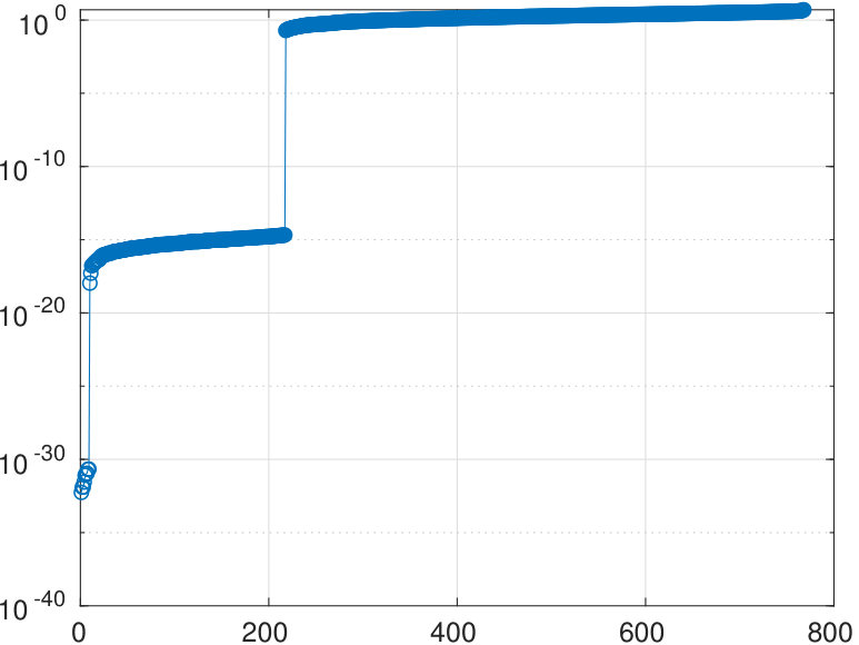 Figure 1
 Figure 2
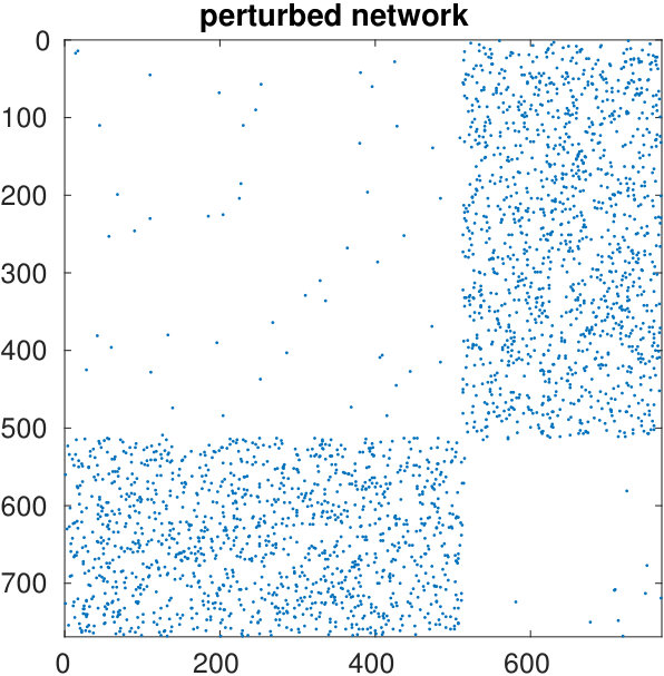 Figure 3
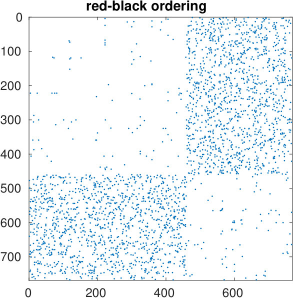 Figure 4
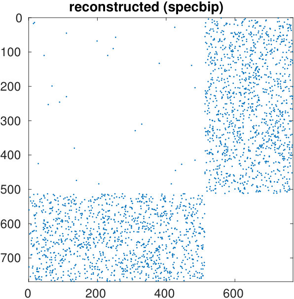 Figure 5
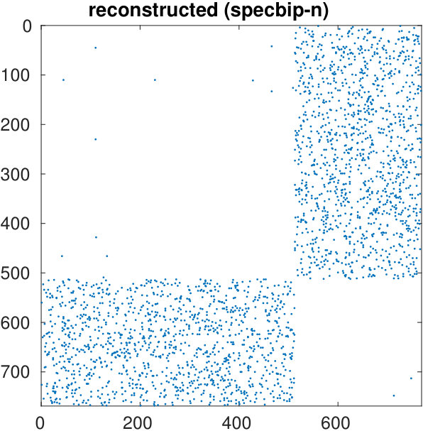 Figure 6
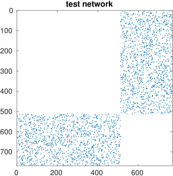 Figure 7
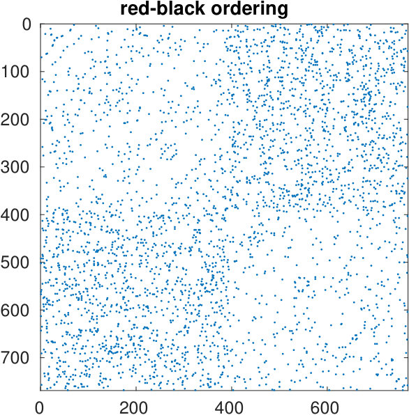 Figure 8
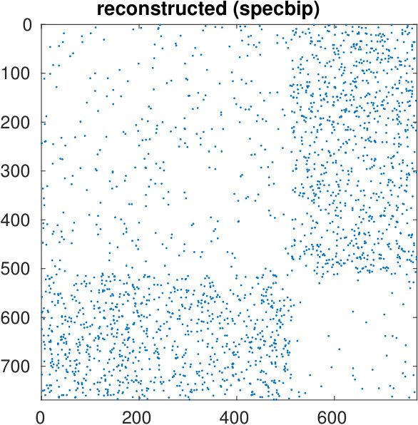 Figure 9
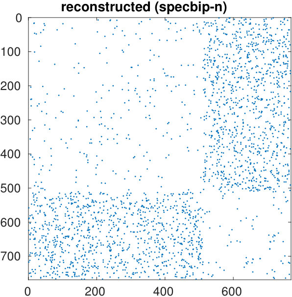 Figure 10
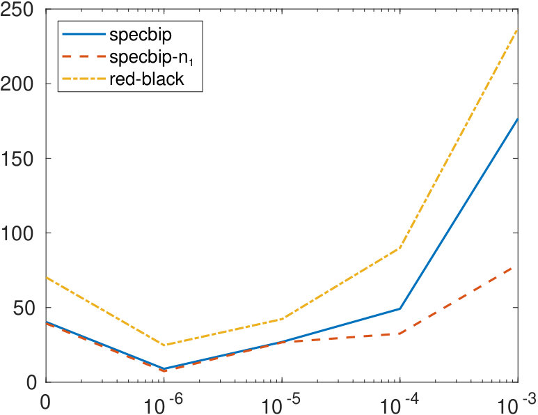 Figure 1
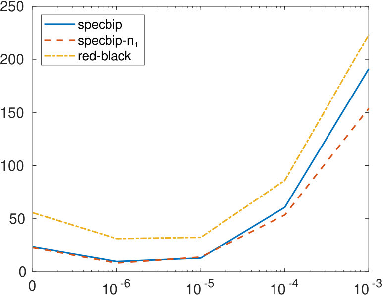 Figure 1
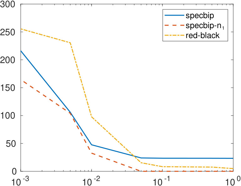 Figure 2
 Figure 2
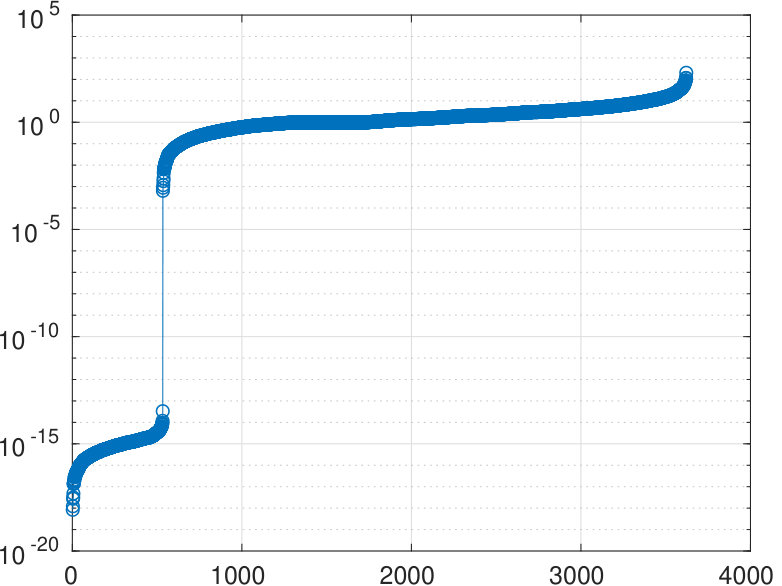 Figure 15
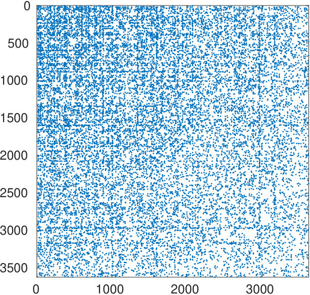 Figure 16
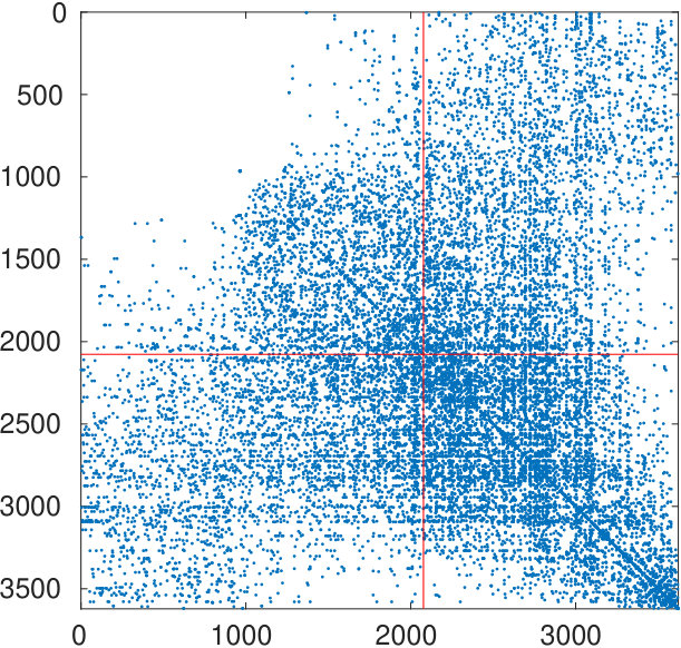 Figure 17
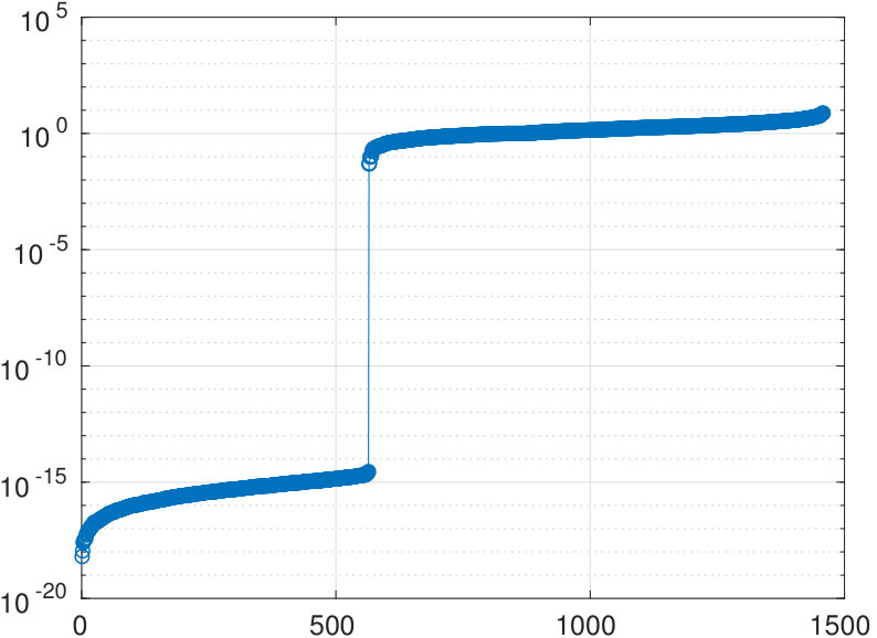 Figure 18
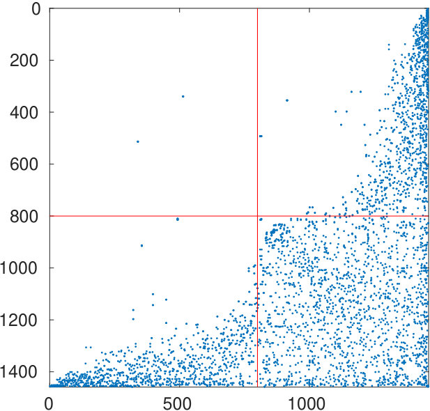 Figure 19
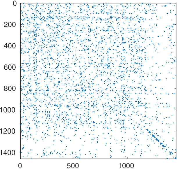 Figure 20
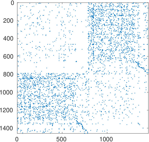 Figure 21
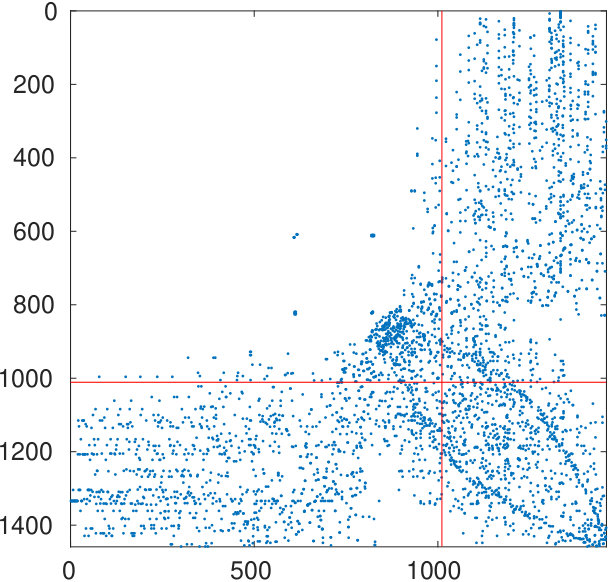 Figure 22
| (256,128) | specbip- | specbip | red-black |
|---|---|---|---|
| 1.22e-16 | 1.89e-16 | 2.33e-03 | |
| 5.46e-04 | 6.74e-04 | 3.72e-03 | |
| 2.80e-01 | 2.79e-01 | - | |
| 1.45e-01 | 1.58e-01 | 2.76e-01 | |
| 4.94e-02 | 5.05e-02 | 3.15e-04 | |
| (512,256) | specbip- | specbip | red-black |
| 1.11e-17 | 1.11e-17 | 2.98e-03 | |
| 1.13e-04 | 1.50e-04 | 3.39e-03 | |
| 4.84e-02 | 6.27e-02 | - | |
| 3.36e-02 | 5.96e-02 | 2.97e-01 | |
| 2.77e-01 | 2.95e-01 | 4.94e-04 | |
| (1024,512) | specbip- | specbip | red-black |
| 7.77e-17 | 0.00e+00 | 4.17e-02 | |
| 9.92e-05 | 2.11e-04 | 4.75e-03 | |
| 1.06e-01 | 1.80e-01 | - | |
| 3.62e-02 | 1.15e-01 | 2.75e-01 | |
| 1.92e+00 | 1.94e+00 | 8.67e-04 |
| (256,128) | specbip- | specbip | red-black |
|---|---|---|---|
| 1.11e-17 | 7.77e-17 | 1.68e-06 | |
| 6.68e-04 | 8.79e-04 | 3.36e-03 | |
| 2.70e-01 | 2.68e-01 | - | |
| 1.23e-01 | 1.49e-01 | 2.58e-01 | |
| 4.39e-02 | 4.70e-02 | 1.01e-03 | |
| (512,256) | specbip- | specbip | red-black |
| 0.00e+00 | 2.22e-17 | 1.40e-04 | |
| 3.05e-05 | 1.91e-05 | 8.81e-04 | |
| 3.88e-02 | 2.38e-02 | - | |
| 1.87e-02 | 1.93e-02 | 3.16e-01 | |
| 2.72e-01 | 2.77e-01 | 5.12e-04 | |
| (1024,512) | specbip- | specbip | red-black |
| 0.00e+00 | 0.00e+00 | 4.04e-03 | |
| 1.91e-07 | 1.03e-05 | 1.07e-03 | |
| 1.73e-04 | 9.49e-03 | - | |
| 9.77e-05 | 9.47e-03 | 3.25e-01 | |
| 1.91e+00 | 1.89e+00 | 9.52e-04 |
| (256,128) | specbip- | specbip | red-black |
|---|---|---|---|
| 0.00e+00 | 0.00e+00 | 7.71e-02 | |
| 0.00e+00 | 5.83e-04 | 1.35e-02 | |
| 2.43e-02 | 4.24e-02 | - | |
| 0.00e+00 | 2.58e-02 | 3.18e-01 | |
| 5.56e-02 | 6.05e-02 | 3.07e-03 | |
| (512,256) | specbip- | specbip | red-black |
| 0.00e+00 | 0.00e+00 | 1.44e-01 | |
| 0.00e+00 | 8.19e-04 | 8.01e-03 | |
| 8.02e-03 | 5.19e-02 | - | |
| 0.00e+00 | 4.47e-02 | 3.31e-01 | |
| 2.77e-01 | 2.76e-01 | 1.08e-03 | |
| (1024,512) | specbip- | specbip | red-black |
| 0.00e+00 | 0.00e+00 | 2.60e-01 | |
| 0.00e+00 | 1.04e-03 | 6.54e-03 | |
| 2.33e-03 | 9.04e-02 | - | |
| 0.00e+00 | 8.71e-02 | 3.28e-01 | |
| 2.02e+00 | 2.07e+00 | 3.99e-03 |
Peer Reviews
No public reviews on file for this paper yet. If you reviewed it on a platform where reviews are public (OpenReview, ICLR, NeurIPS, ICML), you can paste yours below so the community can read it here.
Videos
No videos yet. Explain this paper in a talk, walkthrough, or lecture? Add one.
A spectral method for bipartizing a network and detecting a large
anti-community
A. Concas 111Partially supported by the Fondazione di Sardegna 2017 research project “Algorithms for Approximation with Applications (Acube)” and the Regione Autonoma della Sardegna research project “Algorithms and Models for Imaging Science (AMIS)” (intervento finanziato con risorse FSC 2014-2020 - Patto per lo Sviluppo della Regione Sardegna).222Partially supported by the INdAM-GNCS research project “Metodi numerici per problemi mal posti”.333Anna Concas gratefully acknowledges Sardinia Regional Government for the financial support of her Ph.D. scholarship (P.O.R. Sardegna F.S.E. Operational Programme of the Autonomous Region of Sardinia, European Social Fund 2014-2020 - Axis III Education and Formation, Objective 10.5, Line of Activity 10.5.12).444Member of the INdAM Research group GNCS.
S. Noschese555Partially supported by the INdAM-GNCS research project “Metodi numerici per problemi mal posti”.666Member of the INdAM Research group GNCS.
L. Reichel777Partially supported by NSF grants DMS-1729509 and DMS-1720259.
G. Rodriguez888Partially supported by the Fondazione di Sardegna 2017 research project “Algorithms for Approximation with Applications (Acube)” and the Regione Autonoma della Sardegna research project “Algorithms and Models for Imaging Science (AMIS)” (intervento finanziato con risorse FSC 2014-2020 - Patto per lo Sviluppo della Regione Sardegna).999Partially supported by the INdAM-GNCS research project “Metodi numerici per problemi mal posti”.101010Member of the INdAM Research group GNCS.
Department of Mathematics and Computer Science, University of Cagliari,
Viale Merello, 92, 09123 Cagliari, Italy
Department of Mathematics “Guido Castelnuovo”, Sapienza University of Rome,
P.le A. Moro, 2, I-00185 Roma, Italy
Department of Mathematical Sciences, Kent State University, Kent, OH 44242, USA
Abstract
Relations between discrete quantities such as people, genes, or streets can be described by networks, which consist of nodes that are connected by edges. Network analysis aims to identify important nodes in a network and to uncover structural properties of a network. A network is said to be bipartite if its nodes can be subdivided into two nonempty sets such that there are no edges between nodes in the same set. It is a difficult task to determine the closest bipartite network to a given network. This paper describes how a given network can be approximated by a bipartite one by solving a sequence of fairly simple optimization problems. The algorithm also produces a node permutation which makes the possible bipartite nature of the initial adjacency matrix evident, and identifies the two sets of nodes. We finally show how the same procedure can be used to detect the presence of a large anti-community in a network and to identify it.
keywords:
network analysis , network approximation , bipartization , anti-community
MSC:
65F15 , 05C50 , 05C82.
††journal: Journal of Computational and Applied Mathematics
1 Introduction
Networks describe how discrete quantities such as genes, people, proteins, or streets are related. They arise in many applications, including genetics, epidemiology, energy distribution, and telecommunication; see, e.g., [7, 17] for discussions on networks and their applications. Networks are represented by graphs , which are determined by a set of vertices (nodes) , a set of edges , and a set of positive weights . Here represents an edge from vertex to vertex . The weight is associated with the edge ; a large value of indicates that edge is important. For instance, in a road network, the weight may be proportional to the amount of traffic on the road that is represented by the edge . In this paper, we consider connected undirected graphs without self-loops and multiple edges. In particular, all edges represent “two-way streets,” i.e., if is an edge, then so is . The weights associated with these edges are assumed to be the same. In unweighted graphs all weights are set to one.
We will represent a graph with nodes by its adjacency matrix , where
[TABLE]
Since is undirected and the weights associated with each direction of an edge are the same, the matrix is symmetric. The largest possible number of edges of an undirected graph with nodes without self-loops is , but typically the actual number of edges, , of such graphs that arise in applications is much smaller. The adjacency matrix , therefore, is generally very sparse.
A graph is said to be bipartite if the set of vertices that make up the graph can be partitioned into two disjoint nonempty subsets and (with ), such that any edge starting at a vertex in points to a vertex in , and vice versa. This, in particular, excludes the presence of self-loops in a bipartite graph.
Bipartivity is an important structural property. It has been studied also as the -coloring problem [3]. In fact determining if a graph can be colored with 2 colors is equivalent to determining whether or not the graph is bipartite, and thus testing if a network is bipartite or not is computable in linear time using breadth-first or depth-first search algorithms. It is therefore interesting to determine a bipartite approximation of a non-bipartite graph, or measure the distance of a non-bipartite graph from being bipartite. We say that a splitting of the set of vertices of a weighted undirected graph into two disjoint nonempty subsets and (with ), is a best bipartization of if the sum of the weights associated with edges that point from vertices in () to vertices in the same set is minimal. Such edges are called “frustrated”, and computing the minimum number of edges whose deletion makes the graph bipartite is an NP-hard optimization problem [25]. We remark that the above definition is analogous to the definition of a best bipartization of an undirected unweighted graph proposed by Estrada and Gómez–Gardeñes [8], where the spectral bipartivity index of a network with adjacency matrix is defined as
[TABLE]
This measure also can be applied to the weighted graphs considered in the present paper.
The problem of discovering approximately bipartite structures in graphs and networks has been considered by various authors. Most popular approaches are based on the eigendecomposition of the Laplacian and signless Laplacian matrices. Other spectral approaches consider the adjacency matrix associated to the graph. In the case of a symmetric bipartite adjacency matrix, the signs of the entries of an eigenvector associated with the smallest eigenvalue can be used to partition the graph, i.e., nodes that correspond to positive entries belong to one set, and nodes that correspond to negative entries belong to the other set; see [21]. In case the smallest eigenvalue is multiple, the splitting of the nodes may vary according to the considered vector in the associated eigenspace. In [16] the presence of pairs in the spectrum of the adjacency matrix of a bipartite graph is exploited in order to identify approximated bipartite structures within protein-protein interaction undirected networks; see also [23] for a spectral approach that can be used to discover approximately bipartite substructures in directed graphs.
We are interested in developing a numerical method for determining a “good” bipartization , i.e., a bipartization for which the sum of the weights associated with the edges that point from a vertex in to a vertex in , or vice versa, is fairly small. The algorithm is approximated, or “heuristic”, in the sense that it does not necessarily produce the best possible bipartization.
As it will be made clear in the following, the same bipartization method may be used for the identification of large anti-communities. A community is a group of nodes which are highly connected among themselves, but are less connected to the rest of the network, or isolated from it. Conversely, an anti-community is a node set that is loosely connected internally, but has many external connections [9]; see [10], where a spectral method is used to detect communities and anti-communities. Community and anti-community detection in networks is an important problem with applications in various fields, including physics, computer science, and social sciences [5, 15, 18, 19, 24]. Although the identification of communities is predominant in the investigation of meso-scale structures in networks, the detection of the so-called core-periphery structures, whose most popular notion was developed by Borgatti and Everett [4], attracts a continuing interest also in the mathematical community; see also [20]. For our purposes, the identification of a single large anti-community can be understood as that of a core-periphery structure in the given network.
This paper is organized as follows. Section 2 discusses some properties of bipartite graphs and Section 3 describes an algorithm for determining a “good” bipartization. An application of the bipartization method to the identification of large anti-communities is discussed in Section 4. Finally, Section 5 presents computed examples and two case studies, while Section 6 contains concluding remarks.
2 Approximating the spectral structure of a bipartite graph
This section discusses some properties of the adjacency matrix for an undirected bipartite graph. Some inequalities that are useful for the design of our bipartization method also will be introduced. The discussion in the first part of the section assumes that the vertices are suitably ordered. Subsequently, we will describe how to achieve such an ordering.
Assume for the moment that the undirected graph is bipartite, i.e., its vertex set can be split into two disjoint nonempty subsets and with and nodes, respectively, such that there are no edges between the nodes in and between the nodes in . We may assume that , otherwise we interchange the sets and .
Let the vertices in the set be ordered so that the first of them belong to the set and the remaining vertices belong to . Then the adjacency matrix for the graph is of the form
[TABLE]
where denotes the zero matrix, and with if the node in is connected to the node in ; otherwise .
We adapt to our notation a known result in graph theory; see, e.g., [1, Theorem 3.14].
Proposition 2.1**.**
Let be an unweighted graph with nodes. Then is bipartite and the adjacency matrix can be partitioned as in (2.1) if and only if the spectrum of the adjacency matrix is symmetric with respect to the origin, i.e.,
[TABLE]
for some integers and non-negative numbers . The claim holds true also for weighted graphs, as long as the weights are positive.
Proof.
For the sake of clarity, we give a quick sketch of the proof. The necessary condition is straightforward. The sufficient condition can be proved by noting that, for , if the spectrum is symmetric. Then, the positivity of the weights implies that , that is, the graph is bipartite since it does not contain odd cycles. ∎
Remark 2.2**.**
Under the assumption of Proposition 2.1, it is immediate to verify that if is a nonzero eigenvalue of and , with and , is an associated eigenvector, then is an eigenpair, too. This implies that is a singular value of the block in (2.1), while and are its left and right singular vectors, respectively, if scaled to be of unit length.
Let with . Then, the above observation gives us the possibility to describe the spectral structure of in terms of the singular value decomposition of ; see also [12, Section 8.6.1]. Let be a singular value decomposition of , where has as its upper block, and and are orthogonal matrices with . Introduce the diagonal matrix
[TABLE]
and the orthogonal matrix
[TABLE]
where , , and , with and . Then, the spectral factorization
[TABLE]
takes the form
[TABLE]
In the special case when , the submatrices of (2.3) with columns disappear, and the spectral factorization (2.5) simplifies to
[TABLE]
with .
Now, let be an adjacency matrix of an undirected graph. We would like to approximate the graph by a bipartite one, and therefore seek to approximate by a matrix of the form . We do this in several steps and first show some inequalities that are applicable to diagonal eigenvalue matrices.
Proposition 2.3**.**
Let be a nonincreasing real sequence and let be another real sequence. The distance between these sequences measured in the least squares sense,
[TABLE]
is minimal if and only if the are in nonincreasing order, i.e., if .
Proof.
Assume that both sequences are in nonincreasing order and that the distance can be reduced by changing the order of the . Consider the pairs and . Then
[TABLE]
is equivalent to
[TABLE]
Assume . Then , which is a contradiction unless . If the are ordered arbitrarily, then we can reorder these coefficients pairwise until they form a nonincreasing sequence. Each pairwise swap reduces (2.6). ∎
In our application of Proposition 2.3, we let be the eigenvalues of the adjacency matrix . The graph associated with this matrix might not be bipartite. We would like the sequence of eigenvalues of the matrix , given by (2.1), to be close to the sequence and appear in pairs. By Proposition 2.3, we know that the eigenvalues of should be in nonincreasing order, and by Proposition 2.1 they vanish or appear in pairs. We know from (2.5) that at least eigenvalues of should be zero.
Proposition 2.4**.**
Let , with and , be a real nonincreasing sequence. Then the sequence with elements
[TABLE]
is the closest sequence to in the least squares sense consisting of at least zeros and nonvanishing entries appearing in pairs.
Proof.
The sequence consists of zero values and pairs. Indeed, we have
[TABLE]
and it follows that the sequence is nonincreasing. It remains to establish that the defined by (2.7) are the best possible. Consider the minimization problems
[TABLE]
The solution sequence is given by (2.7). Thus, the form a nonincreasing sequence consisting of zero values and pairs. It is the closest such sequence to the sequence in the sense that it solves the minimization problems (2.8). ∎
We would like to determine an approximation of the matrix by a matrix of the form (2.1), where we allow row and column permutations of the latter matrix. Define the spectral factorization
[TABLE]
where is an orthogonal matrix and the eigenvalues are ordered according to
[TABLE]
We remark that only the first eigenvalues are ordered as in (2.4).
Let us initially assume that the nonzero eigenvalues are distinct. If the eigenvectors are made unique, e.g., by making their first component positive, a comparison with (2.5) shows that
[TABLE]
where is the flip matrix
[TABLE]
In the presence of multiple nonzero eigenvalues, the corresponding eigenvectors are not uniquely determined, so the spectral factorization (2.9) is only one of several possible distinct factorizations.
Let
[TABLE]
be a spectral factorization of with an orthogonal eigenvector matrix and the eigenvalues ordered according to
[TABLE]
Partition the eigenvector matrix conformally with the eigenvector matrix of , i.e.,
[TABLE]
We would like to to approximate the eigenvector matrix of by the eigenvector matrix of . This suggests that we solve the minimization problem
[TABLE]
where denotes the Frobenius norm. This problem splits into the three independent problems
[TABLE]
Problem (2.13) can be written as
[TABLE]
The following result shows how we can easily solve this problem.
Proposition 2.5**.**
The solution of problem (2.16) can be determined by computing the singular value decomposition of and setting all singular values to one.
Proof.
Consider the problem
[TABLE]
It can be written as
[TABLE]
The first and last terms are independent of . Therefore we obtain the equivalent linear minimization problem
[TABLE]
Similarly, the linear problem associated to the minimization problem (2.16) is given by
[TABLE]
Hence, the problem (2.16) is equivalent to determining the closest orthogonal matrix in the Frobenius norm to the matrix . The solution is given by computing the singular value decomposition of and setting ; see [13, Theorem 4.1] for a proof of the latter statement. ∎
The minimization problems (2.14) and (2.15) are solved similarly. This gives the eigenvector matrix in the spectral factorization (2.5).
Remark 2.6**.**
We note that if denotes the singular value decomposition of , then we can express its polar decomposition by
[TABLE]
Since the first factor is the minimizer of (2.17), the deviation of from the identity matrix measures the quality of the approximation.
Remark 2.7**.**
If some of the nonzero eigenvalues of in (2.10) are multiple, the corresponding columns of , , , and , are not uniquely determined. Anyway, when approximating by , and by , those columns contain linear combinations of the previous ones, and so they belong to the same space. Then, the approximations and will make factorization (2.9) valid.
3 A spectral bipartization method
We give here an outline of a spectral bipartization method, based on the above results. It exploits the spectral structure (2.5) of a bipartite graph to determine a node permutation that separates the two sets and , and to construct a bipartite approximation to a connected undirected graph , having a perturbed bipartite structure. The algorithm is exact whenever the input is the adjacency matrix of a bipartite graph, however it has to be considered “heuristic”, as we were not able to prove a complete convergence result for it, apart from the spectrum approximation theorems in Section 2.
There are three problems at hand: estimating the cardinality of the sets and , suitably ordering the nodes in , and, finally, approximating the adjacency matrix by a matrix of the form (2.1). Let be the adjacency matrix of , and assume the spectral factorization
[TABLE]
is available, where is an orthogonal matrix and the eigenvalues are ordered by increasing absolute value.
The first step of our algorithm consists of finding the cardinality and of the two disjoint node sets and , unless they are known in advance. We do this by identifying the number of eigenvalues that are approximately zero.
In principle, this could be done by detecting how many eigenvalues have absolute value larger than a fixed tolerance, but this process is extremely sensitive to the choice of the tolerance. In our numerical experimentation, we found it to be more reliable to detect the largest gap between “small” and “large” eigenvalues.
To do this, we compute the ratios
[TABLE]
Then, for suitably chosen constants and , we consider the index set
[TABLE]
In our experiments, we set and .
An index is in if there is a significant gap between and (), and is numerically nonzero (). If the set is empty, then we are not able to identify a partition of the nodes, and we consider the cardinality of the sets and to be the same. On the contrary, we let be the index defined by
[TABLE]
and set
[TABLE]
where denotes the closest integer to the real number .
The above approach is clearly not completely robust. It is easy to trick it by constructing particular numerical examples, for example by letting in (2.1) have singular values that decay to zero exponentially, or by introducing large gaps in the spectrum of the adjacency matrix. Nevertheless, we found the procedure quite accurate on networks stemming from real-world applications; see, e.g., Figures 6 and 8 in Section 5.
In order to avoid overflow, it may be preferable to use the reciprocal ratios . This is not required in our Matlab implementation, given the features of the programming language. 2. 2.
The subsequent step is to find the sets and , and reorder the nodes. Assume that is bipartite, but that the adjacency matrix corresponds to a random ordering of the nodes, so that
[TABLE]
for a permutation matrix and a matrix of the form (2.1). In this case, the spectral factorization (2.4) becomes
[TABLE]
i.e., the rows of the eigenvector matrix are permuted. In order to recover the structure of the eigenvectors, let us partition the eigenvector matrix as in
[TABLE]
with and .
Assume first that and consider the matrix block . For (2.9) to be valid, the last rows of must vanish. Sorting in descending order the 1-norms of its rows concentrates the smallest entries in the lower block of . Applying the corresponding permutation to the rows of brings this matrix to the form (2.9) and the adjacency matrix to the form (2.1), with the block possibly permuted. When the block is empty, so we consider the matrix . As its first rows should be exactly zero, we sort the 1-norms of its rows in ascending order, and apply the obtained permutation to the rows of . After the reordering, the first nodes are in the set , and the remaining are in the set . We note that applying the permutation to the rows and columns of the initial adjacency matrix highlights the presence in the graph of an approximate bipartite structure. 3. 3.
To finally obtain an approximation of the matrix (2.1) by the computed spectral factorization, we first approximate the eigenvector matrix by solving problem (2.12), and then approximate the eigenvalues in (2.10) by scalars that appear in pairs using Proposition 2.4. Specifically, we let the in the proposition be the eigenvalues (2.11). The defined in the proposition are the eigenvalues of the matrix in (2.5), in the same order.
The above procedure, outlined in Algorithm 1, determines the eigenvectors and eigenvalues of a matrix with the block structure
[TABLE]
where the matrix has real entries. The matrix may have a different number of nonzero entries than . In fact, not all nonzero entries may be positive. We can handle this issue in several ways:
Allow to be an adjacency matrix for a weighted graph with both positive and negative weights.
- 2.
Allow to be an adjacency matrix for a weighted graph with positive weights. We achieve this by replacing the matrix in (3.4) by the closest matrix, , in the Frobenius norm with nonnegative entries. The matrix is obtained from by setting all negative entries to zero.
- 3.
Require to represent an unweighted graph. The closest such matrix in the Frobenius norm to the matrix (3.4) is obtained by setting every entry of to the closest member of the set .
The last procedure is the one adopted in the numerical experiments presented in Section 5.
Algorithm 1 can be applied only to small to medium sized problems, i.e., when it is possible to compute a full spectral factorization of . For larger problems, one may reduce the complexity of the computation by renouncing the third step of the algorithm. Indeed, when is not too large, a partial spectral factorization may lead to constructing a basis for the null space of , that is, to obtaining the matrix . This would allow one to generate the permutation that takes the adjacency matrix to an almost bipartite form, identifying the two sets and .
4 Anti-communities
Let us consider a symmetric matrix of size with a zero leading square block of size . Then, may be considered the adjacency matrix of a network with an anti-community of nodes. The matrix has the form
[TABLE]
with of size and a square matrix of order . In the following, we denote by the null space of , by its range, and by the restriction of the submatrix to .
Theorem 4.1**.**
Let be as in (4.1) and let be partitioned consistently with . Then the equation
[TABLE]
has linearly independent solutions with . Moreover, if
[TABLE]
then there are also linearly independent solutions to with , so that .
Proof.
Let and consider the case . Let us search for vectors such that . Then we have
[TABLE]
Since is of full rank and , it follows from that and, hence, . The latter implies that is in the null space of , which has dimension . Thus, the matrix admits the following linearly independent eigenvectors corresponding to the eigenvalue ,
[TABLE]
where , , are the left singular vectors of . Hence, has multiplicity .
Let us now assume that . Then may or may not have zero eigenvalues. Indeed, for to have a vanishing eigenvalue, the vector that appears in (4.3) has to belong to the null space of , which has dimension . Then, there will be zero eigenvalues if and only if the system
[TABLE]
has a solution.
If instead , i.e., if is nonsingular, then implies that both and . Hence, , and all the eigenvalues of are different from zero.
We finally turn to the case when the submatrix is rank deficient, that is, . The right-hand side of (4.3) is equivalent to
[TABLE]
Let be a nontrivial solution of (4.2). When , there has to be a vector with . Since in this case the null space of has dimension , there are linearly independent solutions of (4.2) with .
The existence of a solution of (4.2) with a nonzero subvector is equivalent to
[TABLE]
This condition does not hold for most matrix pairs . ∎
Remark 4.2**.**
We note that if , then the equation has exactly
[TABLE]
linearly independent solutions.
Theorem 4.1 shows that if a network has a large anti-community (), the spectral decomposition has the form
[TABLE]
The structures of and are very similar to those of and in (2.9), respectively. For this reason, the bipartization algorithm described in Section 3, is able to detect the presence of a large anti-community and to order the nodes so that the adjacency matrix takes the form (4.1). In case a group of nodes is only approximately an anti-community, the algorithm produces an adjacency matrix that approximates (4.1).
To summarize, when , if a network is either bipartite or contains a large anti-community, its adjacency matrix has zero eigenvalues; the converse is not true. If has a multiple zero eigenvalue, then we can recognize the presence of one of the two above cases by observing the structure of the eigenvector matrix.
5 Computed examples
In the following numerical experiments, we fix the integers and , and construct a random matrix of the form (2.1), with a sparse block with density . The matrix is first perturbed, by replacing its (1,1) and (2,2) blocks by sparse matrices of appropriate size and density , and then “scrambled”, by applying the same random permutation to its rows and columns.
We apply the algorithm of Section 2 to the matrix either by supplying the cardinality of the two sets and (this approach is referred to as specbip-), or letting the method estimate and from the data; we refer to the latter approach as specbip. Since the block (1,2) of the matrix returned by the method is generally permuted with respect to the initial test matrix, the rows and columns are reordered according to the original sequence of the nodes. The final reordering allows us to compare the resulting matrix to the test matrix .
Our results are compared to the ones obtained by red-black ordering using the MatlabBGL library [11], a Matlab package implementing graph algorithms. A matrix has a red-black ordering if the corresponding graph is bipartite. To find a bipartite ordering, this software uses a breadth first search algorithm, starting from an arbitrary vertex. The partition of the nodes is determined by forming a group containing all the vertices having even distance from the root, and another group with the vertices at odd distance from the root. This procedure is designed to bipartite networks, not to produce an approximation when the bipartization is not exact.
Figure 1 displays the results for a test matrix with , sparsity , and perturbation . In particular, it reports in the upper row a spy plot of the original test matrix, the perturbed version, with random arcs in the (1,1) and (2,2) blocks, and the permuted matrix that is fed to the bipartization methods. The bottom row shows the reconstructed networks. The specbip- approach, which receives the information about the cardinality of the node sets, produces the matrix closest to the original. The general algorithm estimates the cardinalities , according to the number of “small” eigenvalues; see Figure 2, where the absolute values of the eigenvalues are displayed in nondecreasing order. This algorithm produces a slightly less accurate approximation than the previous one, which is anyway much better than the matrix produced by the red/black ordering.
Figure 3 shows the results for a test matrix similar to the previous one, but with a larger perturbation . The estimation of is inaccurate, but the approximation produced by the specbib methods is quite close to the unperturbed matrix, while the red/black ordering matrix is far from it.
Now, let
[TABLE]
where and are square matrices of size and , respectively, and let denote the number of nonzero elements of . To evaluate the quality of the results, we consider the following three indices
[TABLE]
The first two indices measure the distance of from the adjacency matrix of a bipartite graph; see (1.1) for the definition of . The third index measures the approximation error with respect to the starting bipartite network (2.1). To better evaluate the error in the bipartition, we introduce the fourth index , where is the number of nodes from the set that were incorrectly ascribed to the set .
Tables 1, 2, and 3 report the average values of the above four quality indices over 10 realizations of the random test networks. Three different pairs are considered; each table refers to different densities and ; stands for the execution time in seconds.
A comparison of the tables shows that the spectral bipartization algorithm is always more accurate than the red-black ordering method. At the same time, it is much slower than the MatlabBGL function, as in our experiments we compute the whole spectrum of the adjacency matrix, without exploiting its sparsity. To be competitive with existing methods for large-scale problems, the spectral method should be modified in order to perform its task by suitable iterative methods, in order to take advantage of the structure of the adjacency matrix.
From the tables, it can also be observed that knowing in advance the cardinality of the two sets and leads in some cases to a substantial improvement in the quality of the results.
To further investigate the behavior of the bipartition error, we construct a matrix of the form (2.1), letting and , with a sparse random block having density . After randomly permuting the rows and columns, we apply our algorithms to this matrix, as well as to those perturbed by replacing the (1,1) and (2,2) blocks by a sparse matrix with density . The graph on the left of Figure 4 shows the value of the bipartization error obtained when the three methods are applied to an unweighted graph, the one on the right correspond to a weighted graph. All values are averaged over 10 realizations of the random matrices. Both graphs show that the bipartization determined by our approaches is closer to the correct one, with respect to red-black ordering, with specbip- producing slightly better results. The performance of all algorithms degrades as the perturbation becomes less sparse.
In Figure 5, we display the value of for the same examples, for a fixed , and letting the density of the block take values in . The red-black ordering method is more accurate than the specbip algorithm for very sparse networks, while providing the correct cardinality of the set to specbip- produces the best results.
5.1 The NDyeast network
We illustrate the performance of the spectral bipartization algorithm when applied to the detection of anti-communities by analyzing a case study. The NDyeast network describes the protein interaction network for yeast, each edge representing an interaction between two proteins [14]. The data set is available at [2]. In this section we analyze this network, testing the presence of a bipartization or of a large anti-community.
The NDyeast network has 2114 nodes. There are 74 self-loops (nodes connected only to themselves) and 268 nodes disconnected from the network. The adjacency matrix resulting by removing both the self-loops and the isolated nodes has size , and it has 149 connected components. They were identified by the getconcomp function from the PQser Matlab toolbox [6].
In the case of a reducible adjacency matrix, the spectral bipartization algorithm should treat each single connected component one at a time. Since most of the components in the NDyeast network are very small, often just 2 or 3 nodes, we consider the only component with more than 10 nodes, which has 1458 nodes. We process the reduced adjacency matrix with our bipartization method.
The algorithm determines zero eigenvalues (see Figure 6) and identifies two sets of nodes with cardinalities and .
The starting adjacency matrix is displayed in the top-left spy plot of Figure 7. The top-right plot shows the same matrix after the ordering produced by the spectral bipartization algorithm is applied to its rows and columns. This graph clearly displays that there is a large group of nodes in the NDyeast network that do not communicate much among themselves, that is, an anti-community. In the same graph we show the bipartization detected by the algorithm by means of red lines.
Our algorithm can also be applied by supplying the values of , rather than estimating them from the number of zero eigenvalues. If we do this by setting and , we obtain the bottom left graph in the same figure. It shows that in the group of the first 800 proteins, only four of them directly interact.
The bottom-right graph of Figure 7 displays the result of the red-black ordering method, which does not supply any useful information.
We remark that a data set similar to NDyeast (but different) is available at [2]. It is called simply yeast, it consists of 2361 nodes, and it refers to the paper [22]. By processing this data set with our spectral algorithm, we obtain results very similar to the ones displayed in Figure 7.
5.2 The geom network
We also applied the spectral bipartization algorithm to a weighted graph, namely, the geom network, It is extracted from the Computational Geometry Database geombib by B. Jones (version 2002). Nodes represent authors; the value of the entry of the adjacency matrix is the number of papers coauthored by authors and . The data set is available at [2].
The geom network has 7343 nodes and 11898 edges. After removing 1185 isolated nodes, the network presents 875 connected components, the largest of which has 3621 nodes. We applied the bipartization method to the adjacency matrix associated to this component.
The eigenvalues are displayed in Figure 8: 533 of them are detected as being numerically zero, and the cardinalities of the two node sets are and . The left graph of Figure 9 reports the spy plot of the original adjacency matrix; the graph on the right shows the matrix reordered by the spectral bipartization algorithm. The graph highlights the presence of an anti-community of about 1000 authors, who did not collaborate with each other when writing papers.
6 Conclusion
This paper describes how an approximate bipartization of a given graph can be determined by solving a sequence of simple optimization problems. The technique can also be applied to detect anti-communities. Computed examples illustrate the performance of the method described.
Acknowledgment
The authors would like to thank the referees for comments.
The reference list from the paper itself. Each links out to its DOI / PubMed record.
- 1[1] R. B. Bapat, Graphs and Matrices, Springer, London, 2010.
- 2[2] V. Batagelj and A. Mrvar, Pajek data sets (2006). Available at http://vlado.fmf.uni-lj.si/pub/networks/data/
- 3[3] J. A. Bondy and U. S. R. Murty, Graph Theory with Applications, Macmillan, London, 1976.
- 4[4] S. P. Borgatti and M. G. Everett, Models of Core/Periphery Structures, Social Networks, 21 (1999), pp. 375–395.
- 5[5] L. Chen, Q. Yu, and B. Chen, Anti-modularity and anti-community detecting in complex networks, Inf. Sci., 275 (2014), pp. 293–313.
- 6[6] A. Concas, C. Fenu, and G. Rodriguez, P Qser: A Matlab package for spectral seriation, Numer. Algorithms, 80 (2019), pp. 879–902.
- 7[7] E. Estrada, The Structure of Complex Networks: Theory and Applications, Oxford University Press, Oxford, 2011.
- 8[8] E. Estrada and J. Gómez–Gardeñes, Network bipartivity and the transportation efficiency of European passenger airlines, Physica D, 323-324 (2016), pp. 57–63.