Three-loop Euler-Heisenberg Lagrangian in 1+1 QED, part 1: single fermion-loop part
Idrish Huet, Michel Rausch de Traubenberg, Christian Schubert

TL;DR
This paper calculates the three-loop Euler-Heisenberg Lagrangian in 1+1 QED, focusing on the one-fermion-loop contribution, and develops algorithms to analyze the weak-field expansion coefficients.
Contribution
It introduces new computational methods for weak-field expansion coefficients and combines diagrammatic and worldline formalisms for the first time in this context.
Findings
Coefficients are of the form r1 + r2 * zeta(3) with rational r1, r2.
First two coefficients are computed analytically.
Four additional coefficients are obtained through numerical integration.
Abstract
We study the three-loop Euler-Heisenberg Lagrangian in spinor quantum electrodynamics in 1+1 dimensions. In this first part we calculate the one-fermion-loop contribution, applying both standard Feynman diagrams and the worldline formalism which leads to two different representations in terms of fourfold Schwinger-parameter integrals. Unlike the diagram calculation, the worldline approach allows one to combine the planar and the non-planar contributions to the Lagrangian. Our main interest is in the asymptotic behaviour of the weak-field expansion coefficients of this Lagrangian, for which a non-perturbative prediction has been obtained in previous work using worldline instantons and Borel analysis. We develop algorithms for the calculation of the weak-field expansions coefficients that, in principle, allow their calculation to arbitrary order. Here for the non-planar contribution we…
Click any figure to enlarge with its caption.
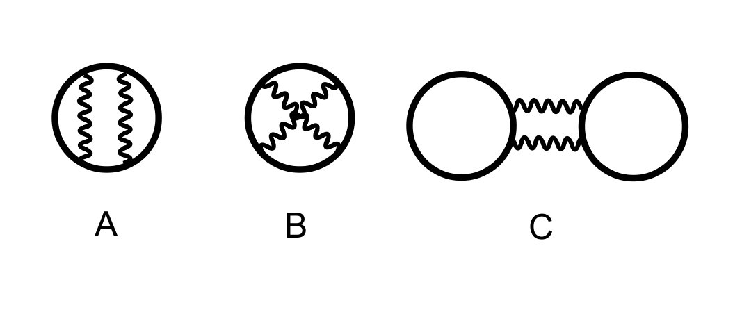 Figure 1
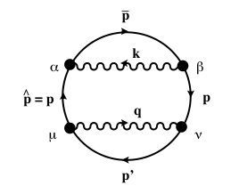 Figure 2
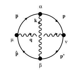 Figure 3
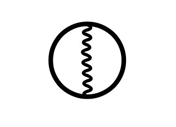 Figure 4
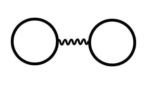 Figure 5
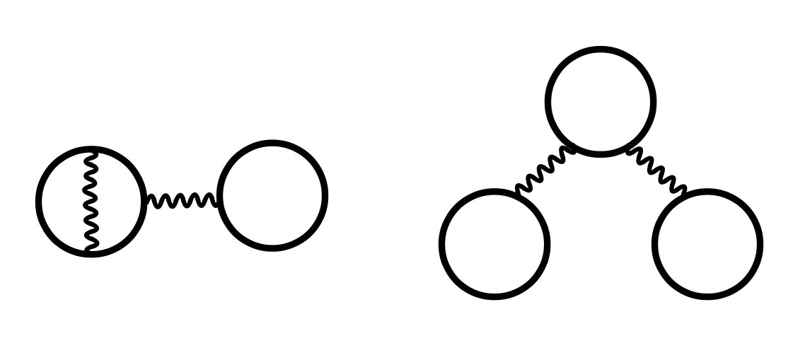 Figure 6
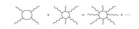 Figure 7
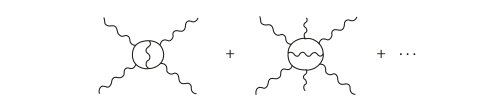 Figure 8
| 0 | ||||||
|---|---|---|---|---|---|---|
| 1 | ||||||
| 2 | ||||||
| 3 | ||||||
| 4 | ||||||
| 5 |
Peer Reviews
No public reviews on file for this paper yet. If you reviewed it on a platform where reviews are public (OpenReview, ICLR, NeurIPS, ICML), you can paste yours below so the community can read it here.
Videos
No videos yet. Explain this paper in a talk, walkthrough, or lecture? Add one.
aainstitutetext: Facultad de Ciencias en Física y Matemáticas, Universidad Autónoma de Chiapas
Ciudad Universitaria, Tuxtla Gutiérrez 29050, Mexicobbinstitutetext: Theoretisch-Physikalisches Institut, Friedrich-Schiller-Universität Jena,
Max-Wien-Platz 1, D-07743 Jena, Germany ccinstitutetext: Université de Strasbourg, CNRS, IPHC UMR7178, F-67037 Strasbourg Cedex, France ddinstitutetext: Instituto de F\́mathfrak{iso}(1,3,\mathbb{C})sica y Matemáticas, Universidad Michoacana de San Nicolás de Hidalgo
Apdo. Postal 2-82, C.P. 58040, Morelia, Michoacan, Mexico eeinstitutetext: Kavli Institute for Theoretical Physics, University of California, Santa Barbara, CA 93106, USA.
Three-loop Euler-Heisenberg Lagrangian in 1+1 QED, part 1: single fermion-loop part
Idrish Huet c
Michel Rausch de Traubenberg d,e
Christian Schubert
Abstract
We study the three-loop Euler-Heisenberg Lagrangian in spinor quantum electrodynamics in 1+1 dimensions. In this first part we calculate the one-fermion-loop contribution, applying both standard Feynman diagrams and the worldline formalism which leads to two different representations in terms of fourfold Schwinger-parameter integrals. Unlike the diagram calculation, the worldline approach allows one to combine the planar and the non-planar contributions to the Lagrangian. Our main interest is in the asymptotic behaviour of the weak-field expansion coefficients of this Lagrangian, for which a non-perturbative prediction has been obtained in previous work using worldline instantons and Borel analysis. We develop algorithms for the calculation of the weak-field expansions coefficients that, in principle, allow their calculation to arbitrary order. Here for the non-planar contribution we make essential use of the polynomial invariants of the dihedral group in Schwinger parameter space to keep the expressions manageable. As expected on general grounds, the coefficients are of the form with rational numbers . We compute the first two coefficients analytically, and four more by numerical integration.
1 Introduction
In one of the first serious computations of early QED, Heisenberg and Euler in 1936 obtained their famous effective Lagrangian induced for a constant electromagnetic field by an electron loop eulhei . For this effective Lagrangian they obtained the following one-parameter integral representation:
[TABLE]
Here and are the mass and proper-time of the electron and the Maxwell invariants, related to the electric and magnetic fields by . The second and third term in brackets implement the renormalization of vacuum energy and charge. The superscript ‘(1)’ stands for one-loop.
This Euler-Heisenberg Lagrangian (‘EHL’ in the following) is to be added to the classical Maxwell Lagrangian, and contains a wealth of information on nonlinear quantum effects such as the field-dependence of the speed of light, vacuum birefringence, and dichroism (see ditgie-book ; dunnerev for reviews). Moreover, it contains this information in a form which is ready for use with standard methods of nonlinear optics. From a particle theory point of view, the EHL holds the information on the one-loop - photon amplitudes for arbitrary in the low-energy limit (see, e.g., itzzub-book ; dunnerev ). In terms of Feynman diagrams, it is thus equivalent to the sum of graphs shown in Fig. 1, where all photon energies are small compared to the electron mass, .
The construction of these low-energy amplitudes from the weak-field expansion of the EHL,
[TABLE]
can, using standard spinor helicity techniques, be carried out explicitly for any number of photons and helicity assignments 56 ; 118 . It turns out that, in this limit, once a helicity assignment has been fixed for all photons, the full dependence of the - photon amplitude on the external momenta and polarization vectors can be absorbed into a single invariant .
Except for the purely magnetic case, the EHL has also an imaginary part related to vacuum pair creation by the electric field component schwinger51 . In the purely electric case, which we will focus on here for simplicity, this imaginary part allows the following decomposition due to Schwinger schwinger51 :
[TABLE]
(). Physically, the th term in this decomposition relates to the coherent production of electron-positron pairs in one Compton volume of spacetime (see, e.g., ritus-ginzburg ). The nonperturbative dependence of these “Schwinger exponentials” on the field supports the interpretation of field-induced pair creation as a vacuum tunneling effect, as envisioned by Sauter as early as 1931 sauter .
The th term in the decomposition (LABEL:schwinger) can be obtained from the th pole in the proper-time integrand of (LABEL:eulhei) by a simple application of the residue theorem. Still, for higher-loop considerations it turns out to be advantageous to observe that the real and imaginary parts of the EHL can be related alternatively through the asymptotic properties of the coefficients of the weak-field expansion (1.2) 37 . In the purely electric case, this expansion is
[TABLE]
where g\equiv\Bigl{(}{eE\over m^{2}}\Bigr{)}^{2} and
[TABLE]
with the Bernoulli numbers. Replacing the weak-field expansion coefficients by their leading asymptotic growth, which is
[TABLE]
one can Borel sum the series. One obtains a Borel integral that is singular, leading to an imaginary part that is precisely the leading term in the Schwinger decomposition (LABEL:schwinger):
[TABLE]
This procedure can be repeated with the subleading, sub-subleading etc. asymptotic growth of the coefficients to reproduce the full Schwinger expansion in (LABEL:schwinger) 37 . However, in this paper we will be concerned only with the leading term in this expansion, which dominates in the weak-field limit.
Our interest here is in multi-loop corrections to the EHL. The two-loop correction to the EHL, involving one internal photon exchange, corresponds to the diagrams shown in Fig. 2 (here it is understood that internal photon corrections are put in all possible ways).
This two-loop EHL was first studied by Ritus in 1975 ritusspin . That calculation, as well as later recalculations ditreu-book ; 18 ; 24 , led to a representation of in terms of rather intractable two-parameter integrals, and so far only the first few coefficients of its weak-field expansion have been computed ritusspin ; 18 ; korsch ; 37 ; 66 .
Schwinger’s formula for the imaginary part (LABEL:schwinger) also generalizes to the two-loop level, in the following way ritusspin ; lebrit ; ritus-ginzburg :
[TABLE]
(). Thus at two-loop one finds the same decomposition into Schwinger exponentials, but the prefactor of the th Schwinger-exponential now is not a constant but a function of the field strength. All that is presently known about these functions explicitly are their leading orders in the weak-field epxansion ritusspin ; lebrit . At this leading order, things become extremely simple: adding up the one-loop and two-loop EHL’s one finds
[TABLE]
And in 37 it was checked, albeit only numerically and based on a calculation of fifteen coefficients, that the method of constructing the imaginary part of the EHL by Borel summation of the weak-field expansion coefficients still works fine at the two-loop level, at least in this weak-field limit. However, it works now in a more complicated manner, since at the two-loop level mass renormalization kicks in. It turns out that, before mass renormalization, the coefficients of have an asymptotic growth that is faster than what we have seen above for the one-loop coefficients; only after adding the counterterm from mass renormalization, which is of the form , and only if is the physically renormalized mass (renormalized at the one-loop level) the addition of the counterterm leads to a cancellation that reduces the leading asymptotic growth of the two-loop coefficients to be precisely the same as at one loop.
Thus the study of the two-loop EHL allows one to understand already two important aspects of the QED S-matrix: first, although the physically renormalized electron mass is usually determined through a calculation of the electron propagator, it can as well be obtained from the effective Lagrangian (although one has to go one loop higher in the perturbative expansion). This has been called “immanent renormalization principle” by Ritus (see, e.g., ritus-ginzburg ). Second, unless the physically renormalized electron mass is used, the two-loop - photon amplitudes dominate over the one-loop ones for sufficiently large , i.e. perturbation theory breaks down already at the two-loop level.
In lebrit it was further noted that, if one would assume that in this weak-field approximation the higher-loop order corrections just lead to an exponentiation,
[TABLE]
then the factor can be absorbed into the Schwinger factor by the following mass-shift,
[TABLE]
This extrapolation, to be called “exponentiation conjecture” in the following, would appear far-fetched if based only on a two-loop calculation, but there is strong independent support for its correctness: first, the same mass shift had been found by Ritus already before for the crossed process of electron propagation in a constant electric field ritusmass . Second, in the vacuum tunneling picture of Sauter-Schwinger pair creation it can be interpreted as taking into account the leading-order Coulomb energy correction due to the fact that the electron - positron pair materializes at a finite distance lebrit . Third, the analogue exponentiation has also been obtained for Scalar QED by Affleck et al. afalma , and using a totally different approach based on a semi-classical approximation to Feynman’s worldline path integral presentation of the multiloop QED effective action feynman50 ; feynman51 .
In 2002 G.V. Dunne and one of the authors 50 ; 51 ; 52 noted that the electric or magnetic backgrounds are by no means the simplest ones in the Euler-Heisenberg context. Computationally, the most favorable case is the one of a (euclidean) self-dual (‘SD’) field. Such a field is defined by , which has the consequence that . For real , the SD effective Lagrangian has properties similar to the magnetic EHL, for imaginary similar to the electric one. Surprisingly, for such a background the EHL turned out to be computable in closed form even at the two-loop level:
[TABLE]
where
[TABLE]
and
[TABLE]
with the digamma function .
This self-dual EHL cannot be realized with real fields in Minkowski space, but still holds physical information on the photon amplitudes, namely on their “all ” helicity components dufish1 ; dufish2 .
Moreover, in the self-dual case the study of the weak-field expansions and the construction of the imaginary parts involve only well-known properties of the digamma function, and thus could be done much more completely and explicitly than for the electric or magnetic case 52 . This made it possible to verify that the above-mentioned construction of the imaginary part by Borel summation works as well at the two-loop level, that is, certain a priori possible complications such as the appearance of additional poles or cuts in the complex plane apparently do not occur in QED.
Having thus gained confidence that the correspondence between the leading asymptotic behaviour of the weak-field expansion coefficients (1.6) and the leading weak-field behaviour of the imaginary part (1.7) of the EHL persists to higher loop orders, it was suggestive to apply this correspondence in reverse to the exponentiation conjecture to gain information on the multiloop photon amplitudes. This was carried out by G.V. Dunne and one of the authors in 60 . There we essentially transferred the factor first from the leading weak-field behaviour of the imaginary part to the leading large - behaviour of the expansion coefficients, and from there to the - photon low-energy amplitudes in the limit of . For the second step it was essential that, as mentioned above, in the low-energy limit the whole kinematical dependence of the photon amplitudes can be absorbed into a single invariant, effectively reducing the amplitude to a single number.
However, this leads to an analytic dependence on , which seems at variance with well-known arguments dyson ; thooftborel that exclude a non-vanishing radius of convergence for generic amplitudes in QED. For a further discussion of this apparent paradox see the recent 111 .
Considering its relevance for the asymptotic structure of the QED perturbation theory, as well as its relation to the vacuum tunneling picture of Schwinger pair creation and the Ritus mass shift, we consider it of the utmost importance to clarify whether the exponentiation really works beyond the two-loop level. However, a calculation of the three-loop EHL seems presently technically out of reach even for the simplest case of a self-dual field.
Now, so far we have focused on spinor QED in dimensions. However, it is important to stress at this point, that spin has not played any role in the above issue. All the statements that we made above about the weak-field expansions at one and two loops hold, qualitatively, as well for Scalar QED ritusscal ; 18 , starting with Weisskopf’s “Scalar EHL” weisskopf ,
[TABLE]
Similarly, at least at the one-loop level the structure of the EHL’s and associated Schwinger exponentials at one-loop is essentially independent of the space-time dimension blviwi ; gitgav . In particular, in dimensions the EHLs become
[TABLE]
where , , and the constant field strength parameter is defined by
[TABLE]
(see app. A for our conventions). We note that the integrals can also be done in closed form, e.g., for the Spinor QED case:
[TABLE]
In 2006 Dunne and Krasnansky studied the Scalar QED EHL in various dimensions at the two-loop level dunkra ; krasnansky and found, in particular, the following explicit formula for this EHL in the case:
[TABLE]
Here is our definition of the fine structure constant in two dimensions, and
[TABLE]
This result is formally very similar to the one above for the EHL in a self-dual background, eq. (1.12), which suggests that QED in two dimensions (scalar or spinor) may be sufficiently similar to serve as a simpler testing ground for the exponentiation conjecture.
But f1irst it had to be established whether the exponentiation conjecture itself admits a generalization to the two-dimensional case. This was settled in 81 where, using the same method of worldline instantons as Affleck et al, it was found that the exponentiation formula (1.10) generalizes to 2D Scalar QED in the form
[TABLE]
By Borel analysis, this leads to the following formula for the limits of ratios of - loop to one - loop coefficients:
[TABLE]
where the expansion coefficients in 2D are defined as
[TABLE]
Thus, differently from the 4D case, in 2D the asymptotic growth of the weak-field expansion coefficients increases with increasing loop level, which presumably is related to the fact that the Coulomb interaction in two dimensions is confining. In 81 it was further shown that the coefficients of the two-loop Scalar QED EHL found by Dunne and Krasnansky, eq. (1.22), indeed fulfill the asymptotic prediction (1.25) with . And there also the corresponding Spinor QED calculation was performed, leading to
[TABLE]
Here is the same function that appeared in the Scalar QED case, eq.(LABEL:defxi2D), and an infrared cutoff that affects only the irrelevant vacuum term. Note that in 2D the Spinor QED EHL has a simpler structure than the Scalar QED one, since it involves the function only linearly. Nevertheless, it is easy to check that the resulting weak-field expansion coefficients obey the same asymptotic relation (1.25). Thus in 2D QED we have an asymptotic prediction for the spinless case, and explicit two-loop computation confirms this prediction and suggests that it does not depend on spin. Moreover, the calculations were significantly simpler than in four dimensions, in particular not requiring mass renormalization; although in 2D QED (finite) mass renormalization exists, it turns out that, differently from the 4D case, the corresponding terms in the EHL do not contribute to the leading order growth of the weak-field expansion coefficients, and thus also not to the weak-field limit of the imaginary part. All this provides strong motivation for pushing the calculation of the EHL in 2D to higher orders.
In this series of papers, we will present a complete calculation of the three-loop EHL in 2D spinor QED. Until recently, it was believed that this effective Lagrangian is (in any dimension) given at the two-loop level by the diagram shown in Fig. 3, and at the three-loop level by the three diagrams shown in Fig. 4. The electron propagators are the full ones in the external field.
However, in 2016 Gies and Karbstein giekar (see also karbstein ; 112 ; 113 ) showed, that also the one-particle reducible diagrams shown in Figs. 5 and 6 have to be taken into consideration.
Previously this type of diagram was believed to vanish, because it contains the one-loop tadpole diagram, which can be shown to formally vanish using momentum conservation and gauge invariance (see, e.g., ditreu-book ; frgish-book ). However, in giekar it was shown that this is not the case any more when it appears as a subdiagram, due to the IR divergence of the photon propagator connecting it to the rest of the diagram in the zero - momentum limit. Thus we will have to include these diagrams here, too.
In this first part of our three-loop analysis we will, however, restrict ourselves to the one-fermion loop (or “quenched”) three-loop diagrams, that is, the diagrams A and B of Fig. 4. These are also the ones most relevant to our main object, the verification of the exponentiation conjecture at the three-loop level.
Partial results of this calculation have been published in various conference proceedings 77 ; 85 ; 108 ; 111 ; 118 . A first attempt at this calculation 77 used the standard approach to this type of calculation, namely Feynman diagrams with the exact electron propagator in the field. The photon propagator was taken in Feynman gauge. Due to the super-renormalizability of 2D QED, at the three-loop level the effective Lagrangian is already UV finite. However, we encountered spurious IR divergences that greatly complicated an already cumbersome calculation. In a second run 85 we used the worldline formalism berkos-prl ; berkos-npb ; strassler1 ; strassler2 along the lines of shaisultanov ; 18 ; 41 ; 41 ; 91 , and also encountered IR divergences. Those could be removed by suitable integrations by parts, but it then was found that it is also possible to avoid the appearance of IR divergences altogether by the choice of a particular covariant gauge. This is the gauge , to be called “traceless gauge” in the following, since it makes the photon propagator traceless in (it had already been used in 81 , but only in the worldline instanton calculation). Returning then to the Feynman diagram calculation, we found that here, too, this gauge makes the IR finiteness manifest, and moreover leads to very significant simplifications due to the identities (3.3), (3.4) below.
Thus both the Feynman diagram and the worldline calculation in this gauge yielded integral representations for diagrams A and B that are manifestly finite term by term. However those representations are quite different: the one from Feynman diagrams is much more compact, while the one from the worldline formalism has the advantage of combining the contributions of the planar and the non-planar diagram, something that would be hard to achieve in the diagrammatic approach. Thus we have chosen to present here both representations, for whatever their worth may be. Since our specific purpose will require a fairly high-order computation of the weak-field expansion coefficients of this Lagrangian, we further show how these coefficients can be obtained from the Lagrangian in an efficient way. Here we use the representation from the diagrammatic approach. As expected on general grounds, the coefficients are of the form with rational numbers , where the comes from the non-planar diagram only. We compute the first two coefficients analytically, and four more by numerical integration.
The organisation of this paper is as follows. In section 2 we calculate the three-loop quenched EHL in the worldline formalism, including also a recalculation of the two-loop EHL. The two-loop EHL had been obtained already in 85 using the Feynman diagram approach, but we include the worldline calculation here because it displays some interesting simplifications. In section 3 we calculate the three-loop quenched EHL again in the diagrammatic approach. Based on the resulting four-parameter integral representation, we present algorithms for the computation of the weak-field expansion coefficients in section 4. Here for the non-planar contribution we make essential use of the high symmetry of diagram B, in two ways: first to develop a certain integration-by-parts procedure, and second to rewrite the integrand in Schwinger parameter space in terms of polynomial invariants of the dihedral group , which helps greatly to keep the expressions manageable. In section 5 we give the results of a calculation of the first six coefficients for both diagrams. Here for the planar diagram A we have analytic results for all six coefficients, while for the incomparably more difficult non-planar diagram B we have computed the first two coefficients analytically, the remaining four numerically. Section 6 gives our summary and outlook. There are four appendices: appendix A gives our conventions. In appendix B we list the momentum integrals appearing in the three-loop worldline calculation. Appendix C contains the corresponding list for the Feynman diagram calculation. Finally, in appendix D we present some elements of the invariant theory of the dihedral group , and sketch the derivation of the basis of invariants used in the weak-field expansion algorithm of diagram B in section 4.
2 Worldline calculation of the quenched three-loop EHL
2.1 Worldline representation of 2-photon and 4-photon amplitudes in a constant field
The starting point for our calculation of the two-loop and three-loop Euler-Heisenberg Lagrangians in the worldline formalism are the following representations of the 2-photon and 4-photon amplitudes in a constant field (see 41 ; 91 for context and derivation of these formulas). Define the field strength tensor by , where
[TABLE]
and further . Introduce the vacuum worldline Green’s functions
[TABLE]
and the generalized (constant field) Green’s functions
[TABLE]
with the scalar, dimensionless coefficient functions
[TABLE]
We note the symmetry properties
[TABLE]
Denote further by
[TABLE]
the field strength tensor associated to photon , and define the “super-bicycle of length ” , involving a subset of the integration variables, by
[TABLE]
Then, the two-photon amplitude in the constant field can be written as
[TABLE]
where is the space-time dimension. We will set from the beginning, since dimensional regularization will not become necessary in our calculation.
Further, let us define the “one-tail” and “two-tail” by
[TABLE]
(, ).
The four-photon amplitude in the constant field can then be written as 91 (omitting the global factor )
[TABLE]
where the upper index on a denotes the “cycle content”:
[TABLE]
Let us mention that each of the sixteen terms appearing in the decomposition (LABEL:defQ) gives a contribution to the four photon amplitude that is separately gauge invariant 26 ; 41 ; 91 .
The representations (LABEL:rep2phot), (2.12) hold mutatis mutandis also in 4D QED, however in the 2D case they are particularly useful, because here all matrices appearing in the above expressions (the ’s and all worldline Green’s functions) commute with each other. This is because in two dimensions all antisymmetric matrices are multiples of each other, and the Green’s functions involve only the matrix . Thus any matrix, or product of matrices, appearing in our calculations below is of the form , which also entails the useful identities
[TABLE]
These simple observations will lead to many simplifications in the following calculations. In particular, the commutativity implies that, for even , the super-bicycles (LABEL:superbicycle) factorize as
[TABLE]
The representations (LABEL:rep2phot), (2.12) hold off-shell, so that the one-loop amplitudes can be used to construct (quenched) higher-loop photon amplitudes by sewing off pairs of photons, say, the photon legs with index and : Using an arbitrary covariant gauge with gauge parameter , this is implemented by setting
[TABLE]
and adding the integration (there is also a combinatorial factor of for each pair of legs).
Thus in the following we will construct the two-loop Euler-Heisenberg Lagrangian from the one-loop vacuum polarization tensor, and the three-loop EHL from the one-loop four-photon amplitude. In the worldline formalism, one could construct these higher loop Euler-Heisenberg Lagrangians also directly using the concept of multi-loop worldline Green’s functions 8 ; 15 ; 41 ; however, this would obscure the decomposition (LABEL:defQ), which we will find very useful in the following. This is because, first, it will allow us to substantially reduce the number of terms in the integrand using the symmetries of the problem; and second, because the gauge invariance term-by-term of this decomposition implies that for each term we can use a different gauge parameter in the sewing procedure (2.17).
2.2 One-loop vacuum polarization tensor in a constant field
Let us start with calculating the vacuum polarization tensor, related to the two-photon amplitude (LABEL:rep2phot) by
[TABLE]
We can simplify this calculation by observing that the constant-field vacuum polarization tensor carries the transversal projector familiar from the vacuum case,
[TABLE]
We note that this is another peculiarity of the 2D case, and due to the fact that no other symmetric and transversal tensor of second degree can be built from , and . In 4D QED the tensor in a constant field involves several independent transversal structures (see, e.g., ditgie-book ).
Thus , and it is sufficient to calculate the trace of , corresponding to the replacement . Making this replacement in , setting , and using (LABEL:superbicycle), we are led to compute
[TABLE]
and
[TABLE]
In the exponent we get
[TABLE]
Putting things together,
[TABLE]
Finally we use, as usual in this type of calculations 41 , the translation invariance of the worldline Green’s functions to put , and rescale . With a further change of variables from to and from to we obtain our final form for the vacuum polarization tensor,
[TABLE]
where now .
2.3 Two-loop EH Lagrangian
We now construct the two-loop EH Lagrangian from the polarization tensor. Using (LABEL:Pispinfin) in the sewing procedure gives (note that )
[TABLE]
Remarkably, after the gaussian - integration all - dependence has already cancelled out, and one is left with a one-parameter-integral:
[TABLE]
We note that the lowest order (f – independent = vacuum) term has an UV divergence at . Subtracting this lowest order term, that is replacing by , we can apply the standard integral formula 51
[TABLE]
Thus we find
[TABLE]
This agrees, up to the irrelevant divergent vacuum term, with the result of the Feynman diagram calculation in 81 that we quoted already in the introduction, eq. (1.27).
2.4 Three-loop quenched EH Lagrangian
We proceed to the construction of the quenched three-loop EH Lagrangians, starting from the worldline representation (2.12) of the one-loop four-photon amplitudes in the field. We apply the sewing procedure (2.17) with and . The universal exponential factor in (2.12) can then be written as
[TABLE]
where
[TABLE]
with
[TABLE]
and
[TABLE]
We will also need the determinant and the inverse of ,
[TABLE]
[TABLE]
In the following we will often treat as numbers matrices which are proportional to the unit matrix, such as .
Further, we observe that, after the sewing, the resulting total worldline integral is invariant under the exchanges , , and . This implies that, of the sixteen terms appearing in the decomposition (LABEL:defQ), only seven are independent and need to be computed; namely, we can now make the replacements
[TABLE]
We will now first work out the effect of the sewing replacements
[TABLE]
on these seven structures. This is simplest for the ones in and ; e.g., in we can use the commutativity of all matrices to write
[TABLE]
In this way, we obtain (independently of ),
[TABLE]
where we have further introduced the abbreviation
[TABLE]
Proceeding to , here we also use to rewrite
[TABLE]
After the sewing of with this gives
[TABLE]
(the term involving drops out here because it contains a factor ).
Coming to the terms in , here things are more delicate. It turns out that, to avoid the appearance of spurious infrared divergences in the integrations, one should use the gauge . This leads to
[TABLE]
where
[TABLE]
and
[TABLE]
The momentum integrals can now be easily performed, without encountering any IR divergences, making them gaussian by exponentiating each denominator,
[TABLE]
The parameter integrals over are convergent since . A list of all integrals is given in appendix B.
The exception is the first term in the square brackets in (2.48) which contains an IR divergence in the integral for any gauge except for our choice ; here care must be taken, and we therefore present its calculation in some detail. We abbreviate and . The from the propagator here cancels against the in the prefactor of (2.48). Thus the integral is finite, and performing it first gives
[TABLE]
The first term in the brackets, which is the IR-critical one, vanishes since , is a linear combination of and , and . In the second term, we can use the identity (2.15) to write
[TABLE]
Thus also the - propagator cancels, and doing the - integral we obtain for the total integral the result
[TABLE]
All the other integrals are straightforward. In this way we arrive at our final result for the quenched part of the three-loop Lagrangian, corresponding to the sum of the diagrams and of Fig. 4:
[TABLE]
where
[TABLE]
where
[TABLE]
Note that in the calculation of we have used the identities (2.14), (2.15), the fact that all matrices are commuting, and that .
Note also that our final integrand is still given in the decomposition corresponding to (2.12),(LABEL:Q3loop), with the subscript on a term denoting its cycle content.
3 Feynman diagram calculation of the quenched three-loop EHL
In this section, we will calculate the quenched part of the three-loop EHL another time, now using the standard formalism. In terms of Feynman diagrams, the quenched part is given by diagrams A and B of figure 4.
3.1 Definitions
We use the 2D electron propagator in a field with constant field strength tensor F=\bigl{(}\begin{smallmatrix}0&f\\ -f&0\end{smallmatrix}\bigr{)}, where . The electron propagator in the field can, using the proper-time representation and Fock-Schwinger gauge, be written as (see appendix A for our conventions)
[TABLE]
where
[TABLE]
(). In the following we will often omit the arguments in and and replace them by superscripts, e.g., . Moreover, we will abbreviate , etc. Greek indices run over the values 1,2 as usual and we use the shorthand . As in our three-loop calculation in the worldline formalism of the previous section, in the Feynman diagram calculation, too, at the three-loop level it turns out to be essential for avoiding spurious IR divergences to take both photon propagators in the “traceless” gauge , where
[TABLE]
In this gauge one has, in and for any , the extremely useful identities
[TABLE]
3.2 Diagram A
We start with the simpler one, diagram A. We parametrize this diagram as in figure 7, with independent momenta , so that the kinematic relations are
[TABLE]
The Feynman rules give for this diagram the following expression:
[TABLE]
Note that this diagram has to be taken twice, and we include this factor in its definition. Applying the identities (3.3), (3.4) (with ) inside the Dirac trace, we can rewrite
[TABLE]
More explicitly, the trace can be written as
[TABLE]
where
[TABLE]
Further, we rewrite the -dependent part of the argument of the exponential by defining
[TABLE]
where we abbreviated , , etc., and defined
[TABLE]
The amplitude is then given by
[TABLE]
where here and in the following is a shorthand for the fourfold - integral.
Working out the traces (LABEL:atraces) and performing the gaussian - integration, one finds
[TABLE]
where
[TABLE]
Here still correspond to , and we have introduced the further abbreviations
[TABLE]
Note that , as required for convergence, and also that .
We now come to the integrals over the photon momenta , and considering the factors of in (3.14), (3.15), it is not obvious that they are IR finite. As was already mentioned, indeed in a general covariant gauge here one would encounter spurious IR divergences. However, this happens not to be the case in traceless gauge; the integrals of are completely finite, and moreover elementary. In appendix C we list all the - integrals needed to complete our calculation of diagram A, as well as of diagram B below.
After these integrations, considerable simplifications occur, leading to the following simple results for :
[TABLE]
Adding up both contributions and taking prefactors into account gives finally the integral representation:
[TABLE]
where we have introduced
[TABLE]
3.3 Diagram B
We come to diagram B, which is expected to be more difficult. See figure 8 for our parametrization.
We again use , , and as the independent variables. The remaining variables are expressed in terms of them as
[TABLE]
With these conventions, the contribution of this diagram is written as
[TABLE]
The Dirac trace in (LABEL:Bexplicit) can again be simplified using (3.3), (3.4). The result can be written as
[TABLE]
where
[TABLE]
Here the term in involving can be dropped since it is odd under the exchange .
For diagram B it turns out to be convenient to first perform the gaussian integral, without even working out the trace appearing in . This integral appears in the form
[TABLE]
where only involves terms with numerators. One can then rewrite the exponent in (3.24) as
[TABLE]
with defined as for diagram A, and
[TABLE]
Any Kronecker - coming out of the integration will belong to , and it will make the trace in vanish on account of the first of the identities (LABEL:idsigma). Therefore the effect of the integration can also be described as a replacement
[TABLE]
Thus for the term we find
[TABLE]
We further abbreviate
[TABLE]
and work out the trace:
[TABLE]
The remaining integrals are again finite and elementary. We rewrite the new exponent in (3.28) as
[TABLE]
where
[TABLE]
again fulfilling .
The five integrals arising from (LABEL:traceB) are included in appendix C. After simple manipulations, one finds the following result for the total momentum integral of :
[TABLE]
For we need only a single integral, given in (C.1a), and leading to
[TABLE]
Putting things together, our final result for diagram B becomes
[TABLE]
where
[TABLE]
4 Calculation of the weak-field expansion coefficients
As was explained in the introduction, our main motivation for this calculation of the EHL in 2D is in the properties of the weak-field expansion. For the one-loop and two-loop contributions, the expansion coefficients have already been obtained in closed form in 81 . In this chapter, we will develop algorithms for the extraction of the three-loop expansion coefficients from the integral representations obtained in the previous two chapters.
In (1.26) we defined the weak field expansion coefficients at loops by
[TABLE]
Thus at three loops, and now introducing, instead of , the expansion variable , we can write
[TABLE]
It will be convenient to replace the coefficients by a new set of coefficients through
[TABLE]
and to denote the contributions of the two diagrams to by , of their sum by .
4.1 Diagram A
The case of diagram A is straightforward. Starting from our final representation (3.18), we rescale etc. Then we can write
[TABLE]
where
[TABLE]
We expand the integrand in powers of ,
[TABLE]
Since
[TABLE]
the coefficients of this expansion can be decomposed into terms of the form
[TABLE]
with and polynomials . After exponentiating the denominator using a Feynman parameter,
[TABLE]
the integrand factorizes in integrals over that are elementary. The integrand of the final - integral consists of terms of the form
[TABLE]
with integer numbers and polynomial numerators . Thus the - integral is elementary, too. This also makes it clear that the coefficients are all rational numbers.
For example, at lowest order we find simply
[TABLE]
leading to
[TABLE]
and to . Using this method, we have found it easy to obtain the first twelve expansion coefficients for diagram A.
4.2 Easy part of diagram B
We proceed to the much more difficult case of the non-planar diagram B. Rewriting again etc. (LABEL:Bfinal) becomes
[TABLE]
where
[TABLE]
with a corresponding rewriting of the functions defined in (3.19), (LABEL:defBCG), defined as in (4.4) and .
We will treat and separately, calling the corresponding contributions to and .
The integration of can still be done using an extension of the factorization method used for diagram A above. Expanding in powers of yields
[TABLE]
where the coefficients can be decomposed into terms of the form
[TABLE]
with
[TABLE]
and polynomials . The factor is exponentiated as in (4.8). In the factor we first rewrite
[TABLE]
and then exponentiate only the second factor:
[TABLE]
After this, the integrand factorizes in integrals over , and these integrals are of the form
[TABLE]
One is left with a double integral over and , involving a product of four Bessel functions and rational factors. Remarkably, MATHEMATICA has an algorithm for the analytic evaluation of this type of integral adamchik . The result is of the form
[TABLE]
with rational numbers . At lowest order one has
[TABLE]
leading to
[TABLE]
At the next order we find polynomials , , , where, for example,
[TABLE]
The full calculation is already too long to be presented here, so let us jump to the final result:
[TABLE]
4.3 Hard part of diagram B
Finding a method of closed-form evaluation for is more difficult. One of the difficulties with its integration is that straightforward attempts will create spurious divergences at . For obtaining a first integral we will make essential use of the high symmetry of this diagram. Namely, while diagram A above has only a invariance generated by the interchanges and , diagram B additionally to those has the symmetry under pair exchange . The group generated by these three reflections is the eight-element dihedral group .
The expansion of
[TABLE]
yields coefficients that can be decomposed in the following way: let us introduce, besides and , now also
[TABLE]
Let us further introduce the basis functions
[TABLE]
Then we can, using , write
[TABLE]
where the and are polynomial functions of the . Here in general the index can take both even and odd values. However, for reasons that will become clear below we shall eliminate the case of odd , multiplying by a factor of in the numerator and the denominator wherever necessary.
Further, the symmetries of diagram B, together with the natural appearance of the variable , motivate us to introduce a differential operator ,
[TABLE]
which is in some sense conjugate to . Its action on is simple:
[TABLE]
Given that is constant under the action of , as far as is concerned and are functions of the single variable . Moreover, they are functions simple enough to be integrated in closed form, for any and an arbitrary number of times. Given that also , we can use integration-by-parts with respect to the variable to write any term of the form appearing in (4.28) as a total derivative with respect to , simply by repeatedly integrating the factors and and differentiating the polynomials until the latter vanish. Denoting by the degree as a polynomial in , and by, e.g., the - fold indefinite integral of in , we can then explicitly write as a total derivative with respect to : , where
[TABLE]
Thus we have now reduced the integrand to boundary terms:
[TABLE]
Moreover, due to the exponential factor there are no contributions from the upper boundaries of the - integrals, and the four contributions from the lower boundaries must be all equal, due to the perfect symmetry of the graph . Thus we can choose to eliminate , and write
[TABLE]
For the remaining three Feynman parameters, we introduce the global scaling variable , and rescale . This leads to the form
[TABLE]
After this rescaling, depends on only through a global factor of :
[TABLE]
Thus the - integral factors out, and we get
[TABLE]
We use the delta function to eliminate , rather than , or , since by the symmetry of diagram the resulting integrand will be symmetric in .
[TABLE]
where we have renamed . We note that at this stage we have the correspondences
[TABLE]
For the computation of the final integral over and in (LABEL:elalphaprime) it will be advantageous to perform a change of variables from to ,
[TABLE]
which yields
[TABLE]
Let us carry through this algorithm for the lowest coefficient . Taking the limit in (LABEL:IB) and eliminating through yields
[TABLE]
where
[TABLE]
For constructing via (4.31) we need
[TABLE]
Going through the steps leading to (LABEL:elalphaprime), we get
[TABLE]
with as in (LABEL:acghfin). After the change of variables (4.37) this becomes
[TABLE]
where now
[TABLE]
Both integrals can be done in closed form, and one finds
[TABLE]
Thus in total we have shown
[TABLE]
In principle, this algorithm after computerization can be used to calculate the weak-field expansion coefficients of to arbitrary order. The problem is that the polynomials and rapidly grow in size with increasing . However, since the complete integrand is invariant under the action of the group , and both and possess this invariance, all those polynomials must be invariant, too (note that this would not be quite true had we permitted odd powers of in the denominator, since itself is only a semi-invariant: it is invariant under and , but changes sign under the pair exchange ). This suggests to improve the algorithm by using the representation theory of the group to rewrite those polynomials more compactly in terms of some basic polynomial invariants of .
As we explain in detail in appendix D, the application of the general theory of polynomial representations of finite groups (see, e.g., benson-book ) to our case of the group , acting on polynomials of four variables, shows that all our numerator polynomials can be rewritten in the form
[TABLE]
where is a polynomial in the four invariants (more precisely semi-invariants, see appendix D) . Of those we have already seen, and the remaining two are defined by
[TABLE]
This choice of a basis of invariants is well-adapted to our integration-by-parts procedure, since but for all get annihilated by .
We are now ready to tackle the case. For one finds
[TABLE]
with coefficient functions that in our new basis read
[TABLE]
It remains now to use (D.18) to eliminate .
The intermediate expressions involved in the integration of are cumbersome, but after following through the algorithm we obtain the final result:
[TABLE]
As a final remark, at high orders it might become useful to give a separate treatment to the denominator since it has full symmetry, while the rest has only symmetry;
We remark that this invariant-based approach could as well be applied to , but it would require a higher-order calculation to see whether this would be more efficient than the method described above.
5 Low-order results
In Table 1 we give the first six coefficients for both diagrams A and B. The coefficients for A and the first two coefficients for B were calculated analytically using the methods developed in the previous section. The remaining coefficients for B were obtained by numerical integration. Note that the coefficients for diagram A are rational, for B of the form with rational numbers .
To the best of our knowledge, there are no results available in the literature that could be used to perform some check on our results. However, let us mention that we have an internal check for the first coefficient, since for this one we had obtained an analytical value already in a previous calculation that used Feynman gauge 77 . In Feynman gauge, we had found
[TABLE]
to be compared with our present result in traceless gauge,
[TABLE]
We see that the sum agrees, , and that the rational part becomes gauge-independent only in the sum over both diagrams, while the - part can come only from the non-planar diagram in any gauge.
Computing a number of coefficients sufficient to address the issues related to the exponentiation conjecture will require a more substantial computational effort, which we leave for future work.
6 Conclusions and Outlook
We have presented here the calculation of the three-loop correction to the Euler-Heisenberg Lagrangian in 1+1 dimensional massive spinor QED. The calculation has been performed in parallel using standard Feynman diagrams and the worldline formalism, treating the constant external field non-perturbatively in both cases. In both formalisms, the use of the “traceless” gauge for the internal photons turned out beneficial in making the IR finiteness of the effective Lagrangian manifest term-by-term. In the Feynman diagram approach, this gauge choice moreover led to substantive simplifications. Both methods led to four-parameter integral representations, although of a quite different structure. The Feynman parameter calculation results in relatively compact integrands, particularly for the non-planar diagram A, while the worldline formalism yields a more extensive integrand, but has the advantage that this integrand holds for both the planar and the non-planar sector. We have further used the worldline formalism for a recalculation of the two-loop EHL that is simpler than the Feynman diagram calculation of 81 .
To the best of our knowledge, this constitutes the first calculation of a three-loop effective Lagrangian in quantum electrodynamics, and also the first three-loop calculation in 1+1 QED (in fact even at the two-loop level the only calculations in 1+1 QED that we have been able to find in the literature are the already mentioned studies by dunkra ; krasnansky for the Scalar QED case, and the recent samsonov on super QED (more effort seems to have gone into exploring the expansion in the mass, see adam-scattering , adam-masspert and refs. therein).
Based on the representation obtained in the Feynman diagram approach, we have developed computerizable algorithms for the analytic calculation of the weak-field expansion coefficients that, in principle, work to arbitrary orders. For diagram B, our algorithm make use of the invariant theory of the symmetry group of the graph, the dihedral group , in a way that may be generalizable to other multiloop graphs and thus of independent interest. As to explicit computation, here we have been satisfied with a low-order test, leaving to future work the task of obtaining a sufficient number of coefficients to confirm or refute the exponentiation conjecture, which is our main motivation for pushing this computation to the three-loop level.
Moreover, the methods developed here should also become useful in an eventual calculation of the three-loop EHL in four dimensions, particularly for the self-dual case which is to some extent a “doubling up” of the two-dimensional case.
Acknowledgements.
We thank Gerry McKeon for early collaboration, and D. Broadhurst, A. Das, G.V. Dunne, R. Jackiw, D. Kreimer, E. Panzer, E. Rabinovici, M. Reuter, and V.I. Ritus for various discussions and/or correspondence. Special thanks to P. Baumann for many explanations on the theory of polynomial group invariants, and to James P. Edwards for performing some independent checks on our Feynman diagram calculations. C. S. thanks CONACYT for support through project Ciencias Basicas 2014 No. 242461, and the Kavli Institute for Theoretical Physics (KITP) of the University of California, Santa Barbara, for hospitality during the program Frontiers of intense laser physics. M. R. thanks the IFM, UMSNH for hospitality. This research was supported in part by the National Science Foundation under Grant No. NSF PHY11-25915. I. H. is thankful to the Theoretisch-Physikalisches Institut of the FSUJ for support while part of this work was completed, funding is acknowledged from CONACyT through the SNI program and PROMEP grant dsa103.5/16/10224.
Appendix A Conventions and formulas for Euclidean 1+1 QED
Dirac equation:
[TABLE]
().
Free electron propagator:
[TABLE]
().
Photon propagator:
[TABLE]
( Feynman gauge, traceless gauge).
Vertex:
[TABLE]
Field strength tensor:
[TABLE]
Fock-Schwinger gauge:
[TABLE]
Electron propagator in a constant field in Fock-Schwinger gauge:
[TABLE]
[TABLE]
().
We use the following straightforward identities:
[TABLE]
().
Appendix B Momentum integrals appearing in the worldline calculation
[TABLE]
have been given in (LABEL:defh).
Appendix C Momentum integrals appearing in the calculation of diagrams A and B
Here we list all the integrals over the photon momenta appearing in the calculations of diagrams A and B in section 3. The parameters should be replaced by the ones defined in (3.16) for diagram A, and defined in (3.31) for diagram B.
[TABLE]
Appendix D Invariants of the dihedral group
Given a finite group and a real dimensional representation (the representation can in fact be also complex) . The representation may or may not be irreducible. The representation induces naturally an action on the set of polynonials with variables . Denoting an dimensional vector of , the action of on is denoted . A polynomial is said to be invariant if for any we have
[TABLE]
The set of polynomial invariants is denoted
[TABLE]
The number of linearly independent polynomial invariants of degree is given by the th coefficient of the Molien series, around zero, of the generating function benson-book
[TABLE]
All polynomial invariants can be expressed in terms of what is usually called primitive and secondary invariants. The number of primitive invariants is equal to the dimension of the representation space, i.e., is equal to sturm-book ; benson-book , so we denote them by . They are algebraically independent, which means that they do not satisfy any polynomial identity of the type . Denote now by the subalgebra of polynomial invariants generated by the primitive invariants. Equivalently can be seen as the set of polynomials in . Denote the degree of respectively. The number of secondary polynomial invariants is equal to decker-book . Denote now the set of secondary polynomial invariants. The set of all invariants are not any more algebraically independent and consequently do satisfy algebraic relations which are called syzygies. It turns out that the subalgebra of invariants is a free module with basis . In particular this means that any invariant can be uniquely written as
[TABLE]
where belongs to , i.e., are polynomials in .
There exist many automated way to compute primary and secondary invariants and we have used the Computer Algebra System for Polynomial Computations called SINGULAR decker-book . Before considering our specific case recall that the polynomial invariants for the dimensional representation of the group of permutation acting on elements consist of the well-known symmetric polynomials. This in particular means that the set of symmetric polynomials of degree is the set of primitive invariants and the only secondary invariant is . In particular taking the notations of the paper we have and and the symmetric polynomials in this case are given by
[TABLE]
The dihedral group is eight dimensional and the three generators in the four dimensional (reducible) representation are given by their action on
[TABLE]
It is obvious to see that not all the s are polynomials invariants for . For the group and for our representation, the Molien series takes the form
[TABLE]
For instance this means that there are linearly independent polynomial invariants of degree six. Since we are considering a representation of dimension four of we must find four primitive invariants. Using SINGULAR, we obtain the primitive invariants
[TABLE]
of degree respectively. Thus the number of secondary invariants is two. Using SINGULAR, the secondary invariant are given by
[TABLE]
Consequently any invariant can be uniquely written in the form
[TABLE]
There is a single syzygy, which is a degree six polynomial equation:
[TABLE]
the set of primitive invariants are and the set of secondary invariants are . We will denote such a set by , where the first entry denotes the degree of the polynomial and the semi-colon separates the primitive from the secondary invariants. This set is however not optimal for our algorithm developed in section 4.3. based on integration by parts with the operator
[TABLE]
since most of the invariants are not annihilated by :
[TABLE]
Further, note that itself is not invariant under the action of the whole group , for instance it changes by a sign under the permutation . Consequently if its action on an invariant polynomial is not vanishing, the resulting polynomial is not an invariant polynomial. In fact, in this case is a semi-invariant polynomial. A semi-invariant polynomial is an invariant polynomial up to a phase (in our case a minus sign) for some of the transformations of . Thus by means of one can associate to any invariant polynomial not in the kernel of , a semi-invariant polynomial. In our case, this suggests to introduce the semi-invariants:
[TABLE]
It is easy to check that the Jacobian of the transformation is non-vanishing, which implies that the semi-invariants are algebraically independent. Now since
[TABLE]
this suggests to consider the new set of primitive invariants of degree respective : , where we have further introduced , which now are all but in the kernel of . Again the Jacobian of the transformation is found not to vanish, so that this new set does not satisfy any polynomial relation and thus constitutes an alternative set of primitive invariants, well-adapted to .
Thus any invariant can now be written as
[TABLE]
with some polynomials and . In this new basis the syzygy is given by
[TABLE]
Since we can further refine the procedure. Introduce which is in the kernel of and using the relationships
[TABLE]
we can eliminate first and then so that the polynomial in (D.16) reduces to
[TABLE]
Here is a polynomial in the variables which are algebraically independent since the Jacobian
[TABLE]
Since the polynomial and are uniquely defined, and since there are no relation between the variables the polynomial is also uniquely defined.
Note that in this “basis” has a non-polynomial expression because we divide by . However this does not matter, since will eventually be replaced by unity anyway in the further procedure of evaluating diagram . The benefit is that now all polynomial invariants are expressed in terms of which are all, except , in the kernel of . This is our optimal “basis”. Note that are invariant polynomials whereas are semi-invariants polynomials. Note also that more precisely depends on and which are invariant under the whole action of the group .
The reference list from the paper itself. Each links out to its DOI / PubMed record.
- 1(1) W. Heisenberg and H. Euler, Z. Phys. 98 (1936) 714.
- 2(2) W. Dittrich and H. Gies, Probing the Quantum Vacuum. Perturbative Effective Action Approach in Quantum Electrodynamics and its Application , Springer Tracts Mod. Phys. 166 (2000) 1.
- 3(3) G.V. Dunne, Cont. Adv. in QCD, 478 (2002), hep-th/0207046.
- 4(4) C. Itzykson and J. Zuber, Quantum Field Theory , Mc Graw-Hill 1985.
- 5(5) L. C. Martin, C. Schubert and V. M. Villanueva Sandoval, Nucl. Phys. B 668 (2003) 335, ar Xiv:hepth/0301022.
- 6(6) James P. Edwards, A. Huet and C. Schubert, Nucl. Phys. B 935 (2018) 198-209, ar Xiv:1807.10697 [hep-th].
- 7(7) J. Schwinger, Phys. Rev. 82 (1951) 664.
- 8(8) V. I. Ritus, “The Lagrangian Function of an Intense Electromagnetic Field”, in Proc. Lebedev Phys. Inst. Vol. 168 , Issues in Intense-field Quantum Electrodynamics , V. I. Ginzburg, ed., (Nova Science Pub., NY 1987).