Simultaneous boundary hitting by coupled reflected Brownian motions
Krzysztof Burdzy

TL;DR
This paper investigates the behavior of coupled reflected Brownian motions, revealing conditions for simultaneous boundary hitting, mutual singularity of local time measures, and specific hitting scenarios in wedge domains.
Contribution
It introduces new phenomena in coupled reflected Brownian motions, including simultaneous boundary hitting and measure singularity, expanding understanding of their boundary interactions.
Findings
Uncountably many synchronized motions can hit the boundary simultaneously.
Local time measures are mutually singular until normal vectors align.
Mirror coupled motions can hit opposite wedge sides at different distances.
Abstract
(i) Uncountably many synchronized reflected Brownian motions can hit the boundary of a domain at the same time. (ii) Measures associated to local times of two synchronized reflected Brownian motions are mutually singular until the time when the normal vectors at the reflection locations become identical. (iii) Mirror coupled reflected Brownian motions can simultaneously hit opposite sides of a wedge at different distances from the origin.
Click any figure to enlarge with its caption.
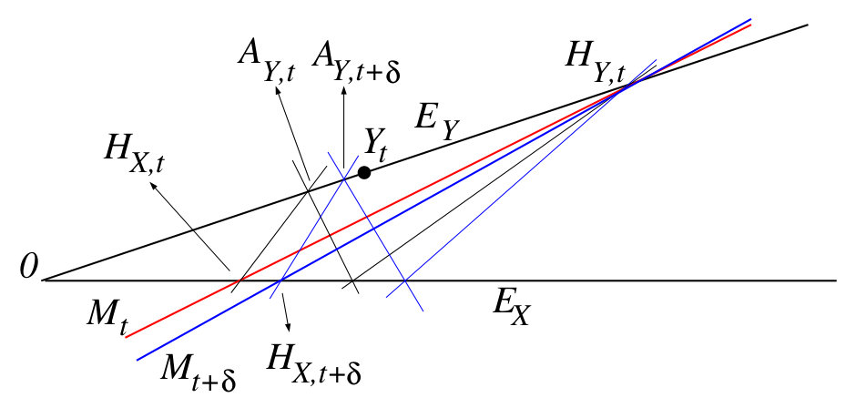 Figure 3
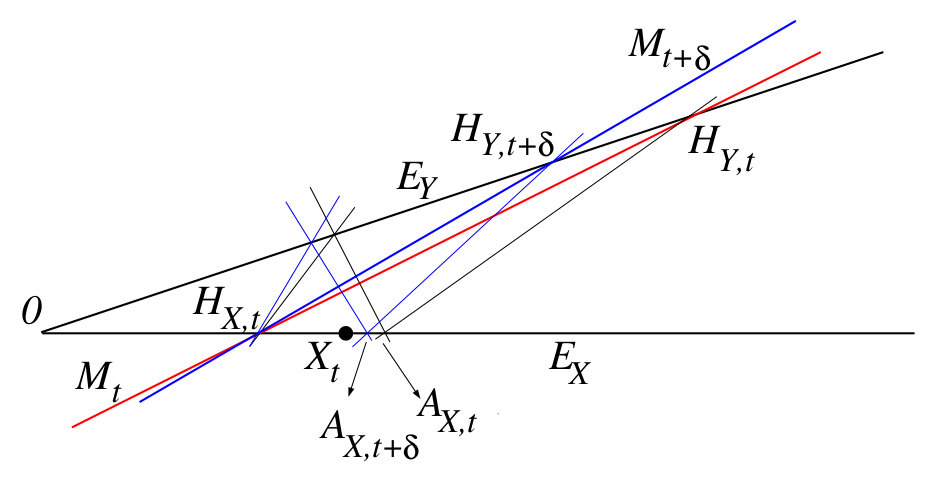 Figure 4
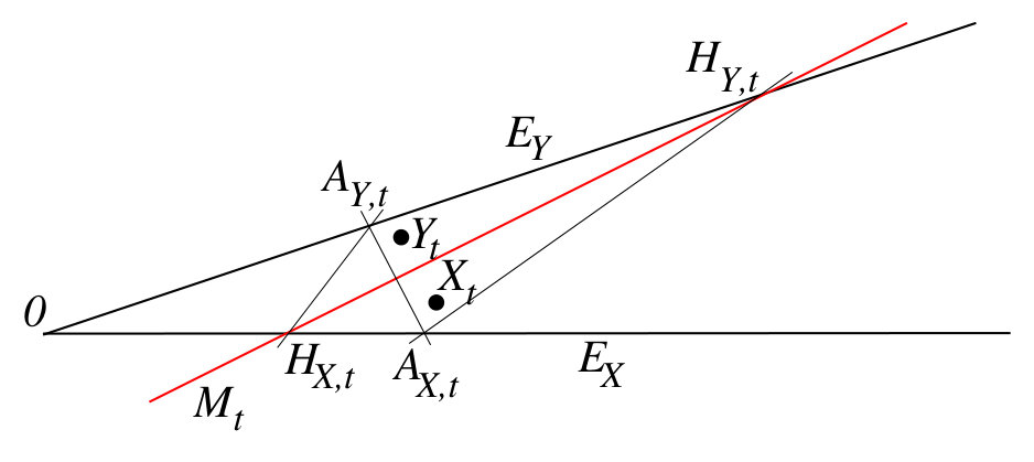 Figure 5
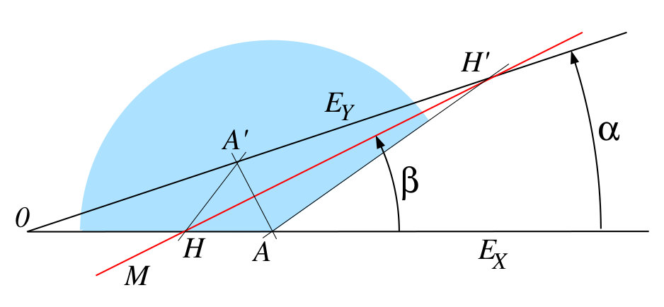 Figure 7
Peer Reviews
No public reviews on file for this paper yet. If you reviewed it on a platform where reviews are public (OpenReview, ICLR, NeurIPS, ICML), you can paste yours below so the community can read it here.
Videos
No videos yet. Explain this paper in a talk, walkthrough, or lecture? Add one.
Simultaneous boundary hitting
by coupled reflected Brownian motions
Krzysztof Burdzy
Department of Mathematics, Box 354350, University of Washington, Seattle, WA 98195
Abstract.
(i) Uncountably many synchronized reflected Brownian motions can hit the boundary of a domain at the same time. (ii) Measures associated to local times of two synchronized reflected Brownian motions are mutually singular until the time when the normal vectors at the reflection locations become identical. (iii) Mirror coupled reflected Brownian motions can simultaneously hit opposite sides of a wedge at different distances from the origin.
Research supported in part by Simons Foundation Grant 506732.
1. Introduction
We will prove three theorems on simultaneous hitting of the boundary by coupled Brownian motions.
The first theorem is essentially known, at least in a weaker form; see [11, 16]. Consider a bounded domain , , and a stochastic flow of reflected Brownian motions starting from all points in , driven by the same Brownian motion. Then, a.s., there is a time such that all processes that started from points in an open non-empty subset of are on the boundary. Our contribution is a new proof based on Brownian cone points.
The second theorem shows that the measures associated with local times of two reflected Brownian motions driven by the same Brownian motion are mutually singular before the time when the normal vectors at the reflection locations are identical.
The third and final theorem is our main result. It is concerned with “mirror” couplings, defined in Section 3. These couplings were used many times to prove theorems in potential theory, see [1, 2, 3, 4, 6, 9]. The main arguments in all of these articles were based on the analysis of the motion of the “mirror,” i.e., the line of symmetry for two coupled reflected Brownian motions. Mirror motion analysis is simple and intuitive as long as a certain simple construction (see Section 3.2) of the mirror coupling can be applied. We will prove that, unfortunately, the simple construction is limited in its scope because two mirror coupled reflected Brownian motions can hit the sides of a wedge at the same time.
2. Synchronous couplings
Let be a bounded connected open set with -smooth boundary, for some . Let denote the unit inward normal vector at . Let be standard -dimensional Brownian motion, , and consider the following Skorokhod equation,
[TABLE]
Here is the local time of on . In other words, is a non-decreasing continuous process which does not increase when is in , i.e., , a.s. Equation (2.1) has a unique pathwise solution such that for all , simultaneously for all (see [14]). For every , the reflected Brownian motion is a strong Markov process. We will call the family a “synchronous coupling.” The construction of reflected paths in [14] is deterministic and dependence on initial conditions is continuous so the function is jointly continuous, a.s. Note that for any and any interval such that and for all , we have for all .
Let denote the open ball with center and radius .
Theorem 2.1**.**
For every ,
[TABLE]
Proof.
For , let
[TABLE]
We will say that is an -cone point for Brownian motion if for all , we have . It follows from the results in [8] that if then cone points exist, a.s. Fix some . Standard arguments based on Brownian scaling and the 0-1 law show that with probability 1, for every there exists an -cone point . Let . By scaling, for every there exists such that for every , with probability greater than , there exists an -cone point such that and for all . Fix an arbitrary and the corresponding . We will assume without loss of generality that .
Since is a bounded domain with a boundary, there exists a point such that . It is easy to see that we can find so small that the following conditions are satisfied.
(i) for all .
(ii) for all .
(iii) If , , and then .
(iv) If and then .
Conditions (i)-(iv) are not logically independent but it is convenient to list them separately for reference.
Fix any . The process is neighborhood recurrent so the stopping time is finite, a.s. Since is continuous, there exists such that
[TABLE]
Let
[TABLE]
By the definition of , the strong Markov property applied at and (2.3), . Since can be any number in , it will suffice to show that if occurred then for all . Fix any and any .
First, we will show that for some . Suppose otherwise. Then and, therefore,
[TABLE]
By the definitions of and , and the assumption that ,
[TABLE]
We use (2.4) and the definitions of and to see that
[TABLE]
Condition (iv) applied to and (2.5)-(2.6) imply that , a contradiction. Hence, for some .
Next we will argue that for . Suppose otherwise and let . If for then because the argument proving (2.5) remains valid if we replace with . This contradicts the definition of so must exist and satisfy . By the definitions of and ,
[TABLE]
This and condition (i) imply that
[TABLE]
We use this bound, definitions of and and assumption that to see that
[TABLE]
It follows from the definitions of and and condition (ii) that this is a contradiction. We conclude that for and, therefore, for .
If then we are done. Suppose that . Recall that we have shown that for some . Let . We have proved that for so . The definition of an -cone point implies that . Since , we obtain
[TABLE]
This, condition (iii) applied with and , and the facts that and for , imply that , a contradiction. We conclude that . ∎
Recall that is a -dimensional domain, for some . We define a measure on by for and .
Theorem 2.2**.**
Consider any , , and let
[TABLE]
Then, with probability 1, the measures and are mutually singular on .
Proof.
Step 1. Let be a cone with vertex 0, with the same angle as that of defined in (2.2), and such that its axis contains , a non-zero vector in . Let denote the angle between vectors and . For non-zero vectors and , let denote the set of times such that for some we have for all .
Suppose that for some , and . We will show that for every . Let . Elementary geometry shows that for every there exist such that if , and then . Fix some and corresponding and . Find so small that for all such that . Let be such that for all . Then
[TABLE]
for all . This implies that , and, therefore,
[TABLE]
Hence, for all . The same argument applies to , so we conclude that for every , one can find such that and for all . It follows that . Next, we will estimate the Hausdorff dimension of all times with this property.
Step 2. The formula for the Hausdorff dimension of “cone points” for planar Brownian motion, derived in [12], is based on the tail properties of the distribution of the exit time from the cone (see especially Corollary 5 of [12]).
In the following, a “cone” is understood in the generalized sense, that is, any set will be called a cone if assuming that and . The rate of decay of the tail of the exit distribution is determined by the first Dirichlet (spherical) Laplacian eigenvalue for the intersection of the cone with the unit sphere (see, for example, Section 1 of [5]). Hence, the Hausdorff dimension of is determined by the first Dirichlet (spherical) Laplacian eigenvalue for the intersection of the cone with the unit sphere. By an argument similar to the proof of Theorem 1.2 of [5], when , the eigenvalues corresponding to converge to . The asymptotic rate of decay for the tail of the exit time from is the same as for the two-dimensional cone with angle . Hence, as , the Hausdorff dimensions of sets converge to , by arguments similar to those given in [12].
For any unit vectors and , let be such that the Hausdorff dimension of is less than . Let , and let be the interior of the set of unit vectors and such that . Note that is open and non-empty.
The set of pairs of unit vectors such that is compact so it is covered by a finite family of sets . It follows that there exists such that the Hausdorff dimension of is less than .
Step 3. We have for all so, by Step 1,
[TABLE]
It will suffice to show that, for any fixed , neither nor charges . Clearly, it is enough to supply a proof for only.
It has been shown in the proof of [7, Thm. 3.2] that for every , the sample path of reflected Brownian motion in a smooth domain is -Hölder, a.s. The same applies to Brownian motion paths so formula (2.1) implies that every component of the vector process is -Hölder, a.s. This in turn implies that is -Hölder, a.s.
Step 2 shows that the Hausdorff dimension of , which we will call , is strictly less than . Consider , integer and a trajectory of such that for some , for all . It follows from the definition of Hausdorff dimension that for every there exists a sequence of intervals , , such that and . This implies that
[TABLE]
Since is arbitrarily small, . Taking the sum over , we obtain . ∎
Remark 2.3**.**
Recall notation from Theorem 2.2. If is a polygonal planar domain and and belong to the interior of the same edge of then for some random time , and measures and restricted to are identical.
3. Mirror couplings
We will present three different constructions of “mirror couplings” of Brownian motions and reflected Brownian motions in planar domains, starting with couplings in the whole plane and then moving to domains of greater complexity. These constructions were originally developed in [10] and later applied in [4] and other articles. Our review is similar to that in [6].
3.1. Mirror couplings in the plane
Suppose that are symmetric with respect to a line and . Let be a Brownian motion starting from , let , and let be the mirror image of with respect to for . We let for . By the strong Markov property applied at , the process is a Brownian motion starting from . The pair is a “mirror coupling” of Brownian motions in the plane.
3.2. Mirror couplings in half-planes
Informally speaking, a mirror coupling in a half-plane is the unique coupling of reflected Brownian motions in the half-plane that behaves exactly as the mirror coupling in the whole plane when both processes are away from the boundary. Suppose that is a half-plane, , and let be the line of symmetry for and . The case when is parallel to is essentially a one-dimensional problem, so we focus on the case when intersects . By performing rotation and translation, if necessary, we may suppose that is the upper half-plane and passes through the origin. We will write and in polar coordinates. The points and are at the same distance from the origin so . Suppose without loss of generality that . We first generate a 2-dimensional Bessel process starting from . Then we generate two coupled one-dimensional processes on the “half-circle” as follows. Let be a 1-dimensional Brownian motion starting from . Let . Let be reflected Brownian motion on , constructed from by the means of the Skorokhod equation. Thus solves the stochastic differential equation , where is a continuous process that changes only when is equal to [math] or and is always in the interval . The process is constructed in such a way that the difference is constant on every interval of time on which does not hit [math] or . The analogous reflected process obtained from will be denoted . Let be the smallest with . Then we let for and for . We define a “clock” by . Then and are reflected Brownian motions in with normal reflection—one can prove this using the same ideas as in the discussion of the skew-product decomposition for 2-dimensional Brownian motion presented in [13]. Moreover, and behave like free Brownian motions coupled by the mirror coupling as long as they are both strictly inside . The processes will stay together after the first time they meet. We call a “mirror coupling” of reflected Brownian motions in half-plane.
The two processes and in the upper half-plane remain at the same distance from the origin. Suppose now that is an arbitrary half-plane, and and belong to . Let be the line of symmetry for and . Then an analogous construction yields a pair of reflected Brownian motions starting from and such that the distance from to is always the same as for . Let be the line of symmetry for and . Note that may move, but only in a continuous way, while the point will never move. We will call the mirror and the point will be called the hinge. The absolute value of the angle between the mirror and the normal vector to at can only decrease.
3.3. Mirror couplings in polygons
We will present an inductive construction of a mirror coupling of reflected Brownian motions in a planar convex polygonal domain based on the constructions presented in Sections 3.1 and 3.2. We will construct a coupling only on a (random) time interval such that or for every .
Assume that , , and let be the mirror coupling of Brownian motions in the whole plane, starting from . Let and .
If and then we let and we end the induction.
Suppose that either or . In the first case let be the edge of to which belongs and let be the line containing . In the second case let be the edge of to which belongs and let be the line containing .
Suppose that , , and have been defined and either or , for some . Let be the mirror coupling of Brownian motions starting from , constructed as in Section 3.2, in the half-plane containing , with boundary . Let .
If and then we let and we end the induction.
Suppose that either or . In the first case let be the edge of to which belongs and let be the line containing . In the second case let be the edge of to which belongs and let be the line containing .
If there is no such that then we let .
We define for by for and such that . If then we extend the definition of to by continuity.
The construction of the mirror coupling can be easily continued beyond under some circumstances. For example, if then and can be continued beyond as a single reflected Brownian motion in .
Let denote the mirror, i.e., the line of symmetry for and . Since the process which hits does not “feel” the shape of except for the direction of , it follows that the two processes remain at the same distance from the hinge on the interval . The mirror can move but the hinge remains constant on the interval . Typically, the hinge jumps at times . The hinge may lie outside at some times.
3.4. Can mirror coupled reflected Brownian motions hit the boundary simultaneously?
The first rigorous construction of a mirror coupling in a domain with piecewise -boundary was given in [2]. The construction given in [2] is rather technical so we find it of interest to determine whether the construction given in Section 3.3 can define a mirror coupling for all in every convex polygonal domain. The positive answer would allow one to analyze the motion of the mirror using the elementary and intuitive methods outlined in Section 3.2. Our main result, given below, says that this is not possible.
Remark 3.1**.**
Before we state our main result, we will list three possible situations when and . It is easy to see that each one of these can occur with positive probability (for an appropriate domain and initial conditions). At the same time they do not pose any technical difficulties with the construction of the mirror coupling. Hence these three situations are not interesting.
(i) It may happen that for some . In this case, one can continue the mirror coupling as a single reflected Brownian motion in representing both and , after time .
(ii) It may happen that and hit the same edge at the same time , at different points. In this case the mirror is orthogonal to at time . One can easily continue the mirror coupling after time , on some random time interval, until one of the processes hits a different edge of .
(iii) If the mirror passes through the intersection point of lines containing two edges and then it may happen that hits and hits at the same time . One can easily continue the mirror coupling after time , on some random time interval, until one of the processes hits a different edge of .
We will use complex and vector notation interchangeably.
Theorem 3.2**.**
Consider a wedge with angle . We will denote the edges of by and . There exist such that if is the mirror coupling of reflected Brownian motions in constructed as in Section 3.3 and then
[TABLE]
Remark 3.3**.**
(i) Recall that if then is defined as . A similar remark applies to .
(ii) It is easy to see that if the event in (3.1) holds then none of the situations listed in Remark 3.1 (i)-(iii) could have occurred at time .
Proof of Theorem 3.2.
Step 1. This step is devoted to a purely geometric lemma. We will investigate the effect of a change of one parameter in a geometric model on another parameter in the same model.
Recall that denotes an angle; we will adopt the convention that all angles are in . For any points and in the plane, let denote the distance between them. We will identify points in the plane with complex numbers and points on the real axis with real numbers. Hence, if is a point in the positive part of the real axis then . Let .
Suppose that , and . Define by . Let be the symmetry with respect to , and define and by and . See Fig. 1.
We will consider and to be constants and we will treat as a variable. Note that and are uniquely determined given and .
Elementary geometry shows that and . By the law of sines,
[TABLE]
Let be the closed wedge with vertex , such that its sides contain and , and lies in its interior. Note that . For and let
[TABLE]
The function takes values in and, informally speaking, sends to . Consider . We use (3.2) to see that
[TABLE]
We use (3.2) once again to get,
[TABLE]
Recall that and fix and such that and . If then . Hence we can find such that if then
[TABLE]
Next we calculate the normal derivative of with respect to the second variable. If we write then
[TABLE]
We will derive an analogous estimate for a mapping corresponding to the other side of the wedge . Let and note that . We will now consider and to be constants and we will treat as a variable. Note that and are uniquely determined given and .
We have . By the law of sines,
[TABLE]
Let be the closed wedge with vertex , such that its sides contain and , and lies in its interior. Let denote the complex conjugate of . For and let
[TABLE]
The function takes values in and, informally speaking, sends to . Consider with . Using (3.7), we obtain
[TABLE]
so, using (3.7) once again,
[TABLE]
Recall that and let and . Then
[TABLE]
If then . Hence we can find such that if then
[TABLE]
We will now calculate the normal derivative of with respect to the second variable. Write . Then
[TABLE]
Recall that and note that for fixed and , we have for ,
[TABLE]
Step 2. Recall that denotes the line of symmetry for and , reflected Brownian motions in . Assume that for some and .
Let () be the straight line containing (). Let and . Let be the symmetry with respect to . In particular, we have for all . Let and be defined by and . Our assumptions on and imply that and . See Fig. 2.
Let be defined by and
[TABLE]
The following definitions apply to .
Let be the closed wedge with vertex , such that its sides contain and , and lies in its interior. For and let
[TABLE]
Let . Let be the closed wedge with vertex , such that its sides contain and , and lies in its interior. Recall that denotes the complex conjugate of . For and let
[TABLE]
It follows from (3.3), (3.8) and (3.12) that
[TABLE]
The function takes values in and sends to . The function also takes values in and sends to .
If for some then we will call both and active at time (and similarly for and ). Suppose that is active at time . Then, over a short time interval , the mirror will move from the position to , the angle will increase to , the wedge will be transformed into the wedge , and the angle of will change from to . As a result, will move to in the direction of (see Fig. 3). Analogous remarks apply to the situation when is active at time (see Fig. 4). For a point between [math] and , its image under will change from to .
Let
[TABLE]
The process is reflected Brownian motion in with (random) oblique reflection, by an argument very similar to the proof of [15, Thm. 2.3]. We will not reproduce that proof here but we will point similarities. In [15, Thm. 2.3], a reflected Brownian motion is transformed by a continuous mapping depending on space and time. In that paper, there is a non-decreasing process, the norm of the original reflected Brownian motion, that is constant on time intervals whose union has full Lebesgue measure. On each of these intervals, the mapping does not depend on time and is analytic in the space variable. In our case, the local times and are constant on time intervals whose union has full Lebesgue measure. On each of these intervals, the mapping does not depend on time and is analytic in the space variable.
The obliquely reflected Brownian motion in has the following representation. For some two-dimensional Brownian motion and ,
[TABLE]
Here is the local time of on . In other words, is a non-decreasing continuous process which does not increase when is in the interior of , i.e., , a.s. The vector of oblique reflection is normalized in (3.17) so that the absolute value of its normal component is equal to 1. The vector is random, i.e., depends on . We will write , for . Hence, . More precisely, if and if .
We will now determine the first component of the vector of oblique reflection . It follows from the construction of the mirror coupling in a half-plane outlined in Section 3.2 that at the time when is active,
[TABLE]
and, therefore,
[TABLE]
Fix some and such that and . Let . We combine (3.5), (3.6) and (3.19) to derive the following estimate for times such that is active,
[TABLE]
Note that .
Let and . Since , we have . Note that . The conditions imposed on and imply that and . Hence, the assumptions (3.9) are satisfied. It follows that we can use (3.10) and (3.11) to derive the following estimate, analogous to (3.20), for times such that is active,
[TABLE]
where .
Let
[TABLE]
It follows from the construction of the mirror coupling given in Sections 3.2-3.3 that on the interval , the distance is non-decreasing, the distance is non-increasing, and the functions and are non-decreasing. This implies that there exist and so small that if
[TABLE]
then for ,
[TABLE]
We will now argue that
[TABLE]
It follows from (3.4), (3.6) and (3.19) that the vector of oblique reflection is locally bounded on the upper boundary of for . The analogous remark applies to the lower boundary of .
Suppose that and . We will show that this leads to a contradiction. The limit exists and is finite because is finite and is a reflected Brownian motion with a locally bounded vector of oblique reflection, hence a continuous process. This implies that either or , hence , according to the definition (3.14) of . This is a contradiction so we conclude that (3.25) is true.
Let . It follows from (3.20), (3.21) and (3.23)-(3.24) that we have the bound if and either or .
It follows from (3.18), a formula analogous to (3.18) for (not stated explicitly), and (3.23)-(3.24) that there exists such that
[TABLE]
Let be so small that if
[TABLE]
then
[TABLE]
Let be so small that
[TABLE]
Assume for a moment that defined in (3.16) is infinite, a.s. It is easy to see that no matter what oblique vector of reflection is, the local time on the boundary increases at a linear rate in the sense that for some , , a.s. This easily implies that there exists such that if the vector of oblique reflection satisfies for and with , and
[TABLE]
then
[TABLE]
It follows that if
[TABLE]
then
[TABLE]
Recall that . We choose such that , and .
The event has probability greater than because of (3.31) and (3.36). Suppose that occurred.
Assume that . We will show that this assumption leads to a contradiction.
Since occurred and ,
[TABLE]
This, (3.22), (3.29) and (3.32)-(3.33) imply that
[TABLE]
This, the assumption that occurred and (3.30) imply that and . Since holds, it follows from (3.27)-(3.28) that and hold. This, coupled with the earlier observations, shows that the event on the left hand side of (3.26) holds with replaced with . Hence, the event on the right hand side of (3.26) holds with replaced with . But this contradicts the definitions of and and the assumption that . The proof that is complete.
The fact that and the definitions of and given in (3.16) and (3.22) imply that and, therefore, . This, in turn implies that (3.37) and (3.38) remain valid. It is elementary to check that . Hence, the fact that implies that . Now it follows from (3.15) that . According to (3.25), . This, the fact that and the definition (3.35) of imply that . Comparing (3.34) and (3.35), and recalling the discussion preceding (3.34), we conclude that , and . We have because . The theorem holds with . ∎
4. Acknowledgments
I am grateful to Zhenqing Chen for the most helpful advice.
The reference list from the paper itself. Each links out to its DOI / PubMed record.
- 1[1] Rami Atar and Krzysztof Burdzy. On nodal lines of Neumann eigenfunctions. Electron. Comm. Probab. , 7:129–139, 2002.
- 2[2] Rami Atar and Krzysztof Burdzy. On Neumann eigenfunctions in lip domains. J. Amer. Math. Soc. , 17(2):243–265, 2004.
- 3[3] Rami Atar and Krzysztof Burdzy. Mirror couplings and Neumann eigenfunctions. Indiana Univ. Math. J. , 57(3):1317–1351, 2008.
- 4[4] Rodrigo Bañuelos and Krzysztof Burdzy. On the “hot spots” conjecture of J. Rauch. J. Funct. Anal. , 164(1):1–33, 1999.
- 5[5] Richard F. Bass and Krzysztof Burdzy. Eigenvalue expansions for Brownian motion with an application to occupation times. Electron. J. Probab. , 1:no. 3, approx. 19 pp. 1996.
- 6[6] Richard F. Bass and Krzysztof Burdzy. Fiber Brownian motion and the “hot spots” problem. Duke Math. J. , 105(1):25–58, 2000.
- 7[7] Itai Benjamini, Zhen-Qing Chen, and Steffen Rohde. Boundary trace of reflecting Brownian motions. Probab. Theory Related Fields , 129(1):1–17, 2004.
- 8[8] Krzysztof Burdzy. Brownian paths and cones. Ann. Probab. , 13(3):1006–1010, 1985.