Composite fermions in Fock space: Operator algebra, recursion relations, and order parameters
Li Chen, Sumanta Bandyopadhyay, Kun Yang, and Alexander Seidel

TL;DR
This paper introduces a second-quantized algebraic framework for composite fermion states, providing recursion relations, operator algebra, and order parameters that deepen understanding of fractional quantum Hall states.
Contribution
It develops a purely second-quantized approach to composite fermion wave functions, generalizing Read's recursion and introducing flux attachment operators and edge excitation algebra.
Findings
Recursion relations for all unprojected Jain CF wave functions
Second-quantized representation of flux attachment operator
Explicit formulas for non-local order parameters
Abstract
We develop recursion relations, in particle number, for all (unprojected) Jain composite fermion (CF) wave functions. These recursions generalize a similar recursion originally written down by Read for Laughlin states, in mixed first-second quantized notation. In contrast, our approach is purely second-quantized, giving rise to an algebraic, `pure guiding center' definition of CF states that de-emphasizes first quantized many-body wave functions. Key to the construction is a second-quantized representation of the flux attachment operator that maps any given fermion state to its CF counterpart. An algebra of generators of edge excitations is identified. In particular, in those cases where a well-studied parent Hamiltonian exists, its properties can be entirely understood in the present framework, and the identification of edge state generators can be understood as an instance of…
Click any figure to enlarge with its caption.
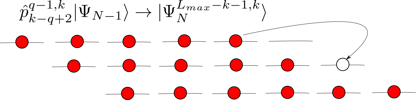 Figure 1
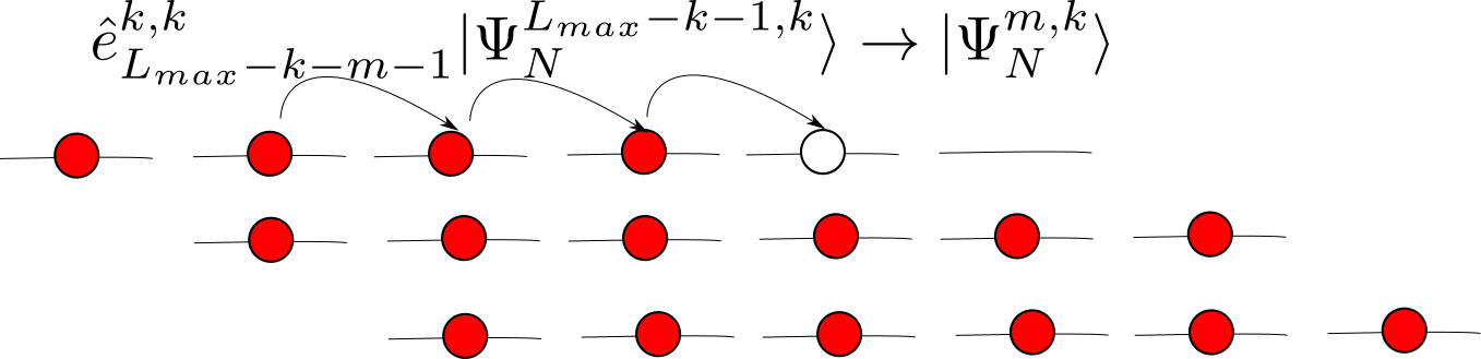 Figure 2
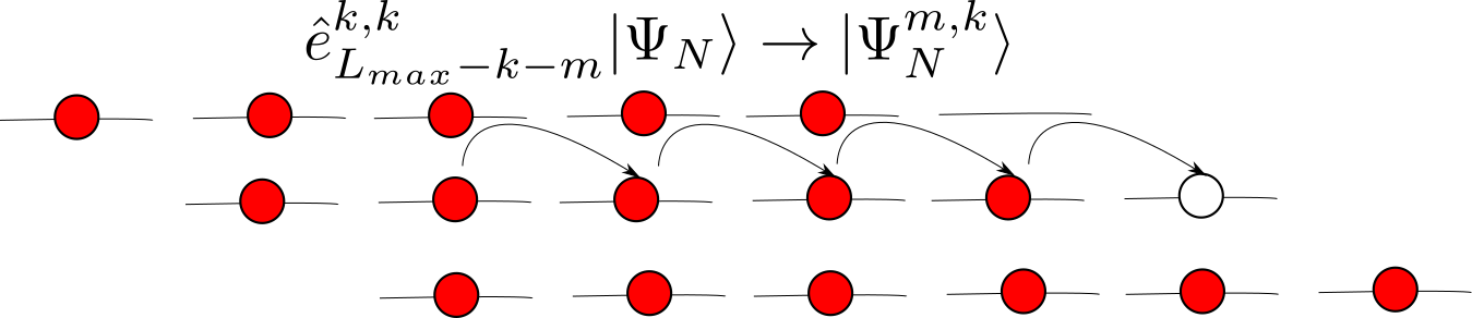 Figure 3
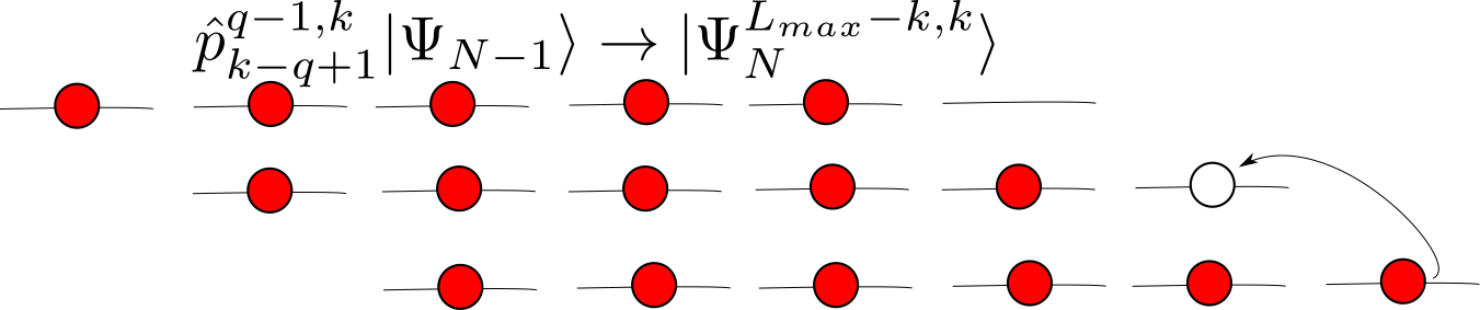 Figure 4
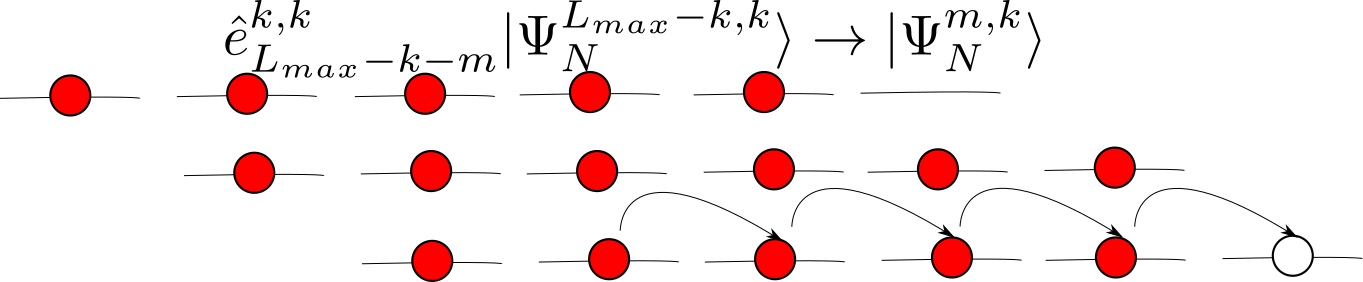 Figure 5
| disk | cylinder | sphere | |
|---|---|---|---|
Peer Reviews
No public reviews on file for this paper yet. If you reviewed it on a platform where reviews are public (OpenReview, ICLR, NeurIPS, ICML), you can paste yours below so the community can read it here.
Videos
No videos yet. Explain this paper in a talk, walkthrough, or lecture? Add one.
Composite fermions in Fock space: Operator algebra, recursion relations, and order parameters
Li Chen
National High Magnetic Field Laboratory and Department of Physics, Florida State University, Tallahassee, Florida 32306, USA
College of Physics and Electronic Science, Hubei Normal University, Huangshi 435002, China
Sumanta Bandyopadhyay
Department of Physics, Washington University, St.Louis, Missouri 63130, USA
Kun Yang
National High Magnetic Field Laboratory and Department of Physics, Florida State University, Tallahassee, FL 32306, USA
Alexander Seidel
Department of Physics, Washington University, St.Louis, MO 63130, USA
Abstract
We develop recursion relations, in particle number, for all (unprojected) Jain composite fermion (CF) wave functions. These recursions generalize a similar recursion originally written down by Read for Laughlin states, in mixed first/second-quantized notation. In contrast, our approach is purely second-quantized, giving rise to an algebraic, “pure guiding center” definition of CF states that de-emphasizes first-quantized many-body wave functions. Key to the construction is a second-quantized representation of the flux attachment operator that maps any given fermion state to its CF counterpart. An algebra of generators of edge excitations is identified. In particular, in those cases where a well-studied parent Hamiltonian exists, its properties can be entirely understood in the present framework, and the identification of edge state generators can be understood as an instance of “microscopic bosonization”. The intimate connection of Read’s original recursion with “non-local order parameters” generalizes to the present situation, and we are able to give explicit second-quantized formulas for non-local order parameters associated with CF states.
I Introduction
Several years after Laughlin’s seminal wave function [1] and subsequent hierarchical constructions [2, 3] opened the door for a theoretical understanding of the fractional quantum Hall (FQH) effect, Jain discovered what can be understood as the essential weakly interacting degrees of freedom under a large variety of circumstances: the concept of a “composite fermion” [4, 5] with no/residual interactions [6, 7, 8] offers a compelling way to predict almost all of the observed plateaus in the lowest Landau level (LL), and has served as the basis for important field theoretical developments [9]. At the same time, reservations regarding the very definition of a composite fermion have been voiced [10]. At a technical level, it is usually defined as a prescription for the construction of variational states via flux attachment, or interchangeably, the attachment of “zeros” or “vortices.” This somewhat operational definition is of course in good keeping with tradition in the theory of the FQH effect, which is to give prescriptions for the variational construction of first-quantized many-body wave functions.
In this work, we wish to depart from this tradition. There is an alternative school of thought in the microscopic study of FQH systems that runs counter to the idea of describing states through analytic functions of coordinates. In a strong magnetic field, activation of degrees of freedom associated with dynamical momenta is energetically costly. These degrees of freedom can therefore be considered either completely or largely frozen out. The physics thus takes place in a reduced Hilbert space that is, to large degree or entirely, stripped of dynamical momenta. This reduced Hilbert space is too coarse to allow for the concept of a position with continuous spectrum. As the orbitals in any given LL may be labeled by an integer, this Hilbert space is properly thought of as associated to a one-dimensional lattice, with the retained LLs (if more than one) interpreted as an internal degree of freedom. The particle position, once projected onto this Hilbert space, is an operator associated to the classical guiding center coordinate (at least in the limit of only the lowest LL kept). Its components have non-trivial commutation relations. Some approaches to the physics in the FQH regime eschew the use of analytic wave functions in favor of working directly with the algebra of these guiding-center coordinates (e.g., Refs. 11, 12, 13). Here, we wish to give a characterization of the concept of a composite fermion using such an approach.
In the past, we have found fruitful a setting in part motivated by certain varieties of multilayer graphene [14, 15, 16], and in part by an interesting class of parent Hamiltonians [17, 18, 19]. Here, the lowest Landau levels are taken to be degenerate, and a local interaction is imposed to stabilize model FQH wave functions within the degenerate LL subspace. These interacting Hamiltonians are extraordinary in that there exists a scheme to infer the long distance physics of the state that is both compelling and simple, and leaves very little room for ambiguity. They unambiguously define a “zero mode space” of elementary excitations, and the counting of such zero modes at given angular momentum (relative to the ground state) tends to exactly match the mode counting in a conformal edge theory. Whenever this applies, we will say that the FQH parent Hamiltonian in question satisfies the “zero mode paradigm.”
There are, of course, many such interesting Hamiltonians known for the case [20, 21, 22, 23]. In this case, some of us have recently shown [24, 25, 26] (for the simplest, Laughlin state parent Hamiltonians) that the rigorous characterization of the zero mode space may be done in a purely second-quantized framework that does not reference the analytic polynomial wave functions of the traditional approach at all. These developments were very useful for the study of the case , which we argued [27, 28] is absolutely necessary to consider if we wish to establish a zero mode paradigm for a more representative set of FQH states. Indeed, already for the phases described by Jain states, which are elemental to both theory and experiment, we argued that a zero mode paradigm requires , with the case extensively discussed in Ref. 27, where a suitable amalgam of first- and second-quantized methods was adopted. The utility of this mixed first/second-quantized formalism was further demonstrated in Ref. 28, where the notion of an “entangled Pauli principle” was introduced, and much of the low-energy physics of the non-Abelian, mixed-Landau-level Jain 221 state [29, 5, 16] was linked to properties of its microscopic two-body parent Hamiltonian.
Here we want to again adopt the “purist” point of view of Refs. 24, 25, 26 and describe unprojected, i.e., mixed-Landau-level composite fermion states in a purely algebraic, second-quantized framework, using operators that are all manifestly expressible in terms of electron creation/annihilation operators referring to some preferred LL basis. In particular, we wish to give such an algebraic definition to the composite fermion and the associated “vortex-attachment” concept itself, within the unprojected, mixed-LL setting described above. In doing so, we simultaneously make contact with second-quantized recursion formulas, in particle number , for Jain-type composite fermion states. This again naturally extends work by some of us on the Laughlin state(s) [24, 25, 26]. Moreover, such recursion formulas turn out to be intimately tied to the concept of an order parameter as discussed by Read [30]. This has the added benefit that we are able to give explicit second-quantized formulas for such order parameters.
The remainder of this paper is organized as follows. In Sec. II we develop the backbone of the formalism for the lowest Landau level only. We develop a second-quantized algebra closely related to symmetric polynomials, following earlier work. We use this to define the composite fermion “flux-attachment” operator in second-quantization, Eq. (13). In particular, we develop a recursion relation for this operator that also clarifies its relation to power-sum, or alternatively, elementary symmetric polynomials. From this we rederive a recursion relation [25] for the Laughlin state. In Sec. III, we generalize all these results to a general number of Landau levels, resulting, in particular, in recursion relations for the second-quantized Jain composite fermion states, Eqs. (49)-(52). The algebra of symmetric polynomials is replaced with a larger algebra of so-called “zero-mode generators,” Eqs. (38)-(40). In Sec. IV, we specialize to two Landau levels, simplifying some of the more general results. In Sect. V and VI, we elaborate on implications of our results in the presence of special parent Hamiltonians and in particular for the zero mode structure of such Hamiltonians. For the special case of filling factor , some earlier conjectures are proven. The algebra of zero-mode generators, while arising in a microscopic setting, is shown to encode the effective edge theory. In Sec. VII, we use the formalism constructed in preceding sections to give explicit expressions for -component non-local order parameters for composite fermion states discussed by Read [31] in terms of the microscopic electron operators [Eqs. (75) and(77)]. We conclude in Sec. VIII.
II Derivation of recursive formula in the lowest Landau level
The heart of this paper will be a second-quantized formula, recursive in particle number , for the composite fermion vortex attachment operator
[TABLE]
where is an even number that we will usually leave implicit, the are the particle’s complex coordinates, and we leave room for a (-dependent) normalization factor that we will not be interested in. For pedagogical reasons, we will begin our discussion by focusing on the lowest LL () in this section. A second-quantized recursion relation for the Laughlin state was given earlier in Ref. 25. The main difference between the latter and the developments in this section will be that here we establish the recursion directly for the Jastrow vortex-attachment operator itself. This will descend to the earlier recursion for the Laughlin state. However, the extension to the operator will prove essential to the generalization of the recursion formulas to unprojected Jain states (the case ).
Considering for now , recall that the -particle Laughlin state may be written as
[TABLE]
where is an integer quantum Hall state for fermions, and the Bose-Einstein condensate for bosons, we will see that a recursion of will descend to a recursion of the Laughlin state. (Here, denotes the vacuum state.) Analogous statements will be true for (Jain states).
The object in Eq. (1), can be interchangeably viewed as an operator and as a symmetric polynomial in variables. As such, it can be written as or (we will stick to the latter), where the are power-sum symmetric polynomials. As a by-product, we will clarify the relation between and such power-sum symmetric polynomials, again via recursion. At operator level, we may then also write
[TABLE]
where the are operator representations of the that facilitate the multiplication of first-quantized wave functions with the symmetric polynomial . Such representations have been discussed at some length in Refs. 24, 25, 26. They depend slightly on the geometry (and LL basis), where, with the conventions of the “thick cylinder”, one simply has
[TABLE]
In this section, we will adopt these thick cylinder conventions for simplicity. Other geometries differ from the above only by normalization conventions that can be implemented via the replacements
[TABLE]
which can be facilitated via the similarity transformation , . We give the normalization constants for various relevant geometries in Table 1. The electron creation/annihilation operators , refer to lowest LL orbitals with angular momentum about the quantization axis. The results in this section will be stated in a manner that is valid for both bosonic as well as fermionic commutation relations, except where explicitly stated otherwise. The sum in Eq. (4) is generally unrestricted, but we will use the convention for for the cylinder and disk geometry (thus rendering the cylinder “half-infinite”), and analogous appropriate restrictions for the sphere. It should be emphasized that for many of our purposes, the “first-quantized” interpretation of the operators Eq. (4) as power-sum symmetric polynomials does not matter, but indeed the definition (4) and the resulting algebraic properties are all that we need. For example, it is trivial to verify that the operators (4) all commute ( !). However, whenever definiteness is required, the term “symmetric polynomial” means a polynomial in the complex coordinates only in disk geometry. On the cylinder, it means a polynomial in the quantities , where is the inverse radius of the cylinder. Analogous statements can be made for the spherical geometry, which we will not use explicitly in this work, but refer the reader to Ref. 24 for further details in this context. The reader who wishes to focus on the disk should always have the substitutions (5) in mind, which do not affect any of the following algebra.
According to a well-known theorem in algebra, any symmetric polynomial in variables can be uniquely expressed through a polynomial in (). This includes the for . Note, however, that the operators Eq. (4) are defined for *any * particle number , and the aforementioned polynomial relations between the and the carry over to the only within subspaces of particle number . Similarly, it is convenient to define , which, for fixed particle number , can be viewed as representing a constant (degree zero) polynomial.
Alternatively, any symmetric polynomials in variables can be generated from elementary symmetric polynomials , , i.e., , with a polynomial. Again, we may ask what second-quantized operator facilitates multiplication with . These are [25, 26]
[TABLE]
given here again for the simple thick cylinder conventions, with disk conventions as detailed in Eq. (5) and Table 1. It is worth noting that unlike the , the vanish automatically for . This is respected by the operators , which automatically vanish on any state with particle number . The and the are related by the Newton-Girard formulas,
[TABLE]
These can be directly derived [26] from the operator definitions (4) and (6), without any reference to the “polynomial interpretation” of these operators. Clearly, Eq. (7) is invariant under the similarity transformation leading to Eq. (5), and is thus seen to be geometry independent even if we did not know about its meaning in terms of polynomials. Eq. (7) may first be used for to express all through . Subsequently, letting , it can be used to explicitly obtain the identities for the in terms of the mentioned above, valid within the subspace of particle number . Independent of , it is also obvious from these relations that the commute with one another (as the do), and also commute with all of the (for the same reason).
We will now derive a second-quantized recursive formula for , which turns out to be straightforward to generalize to higher Landau levels. At the polynomial level, we will also clarify the relation between the Laughlin-Jastrow factor Eq. (1) and power-sum symmetric polynomials. More precisely, we will give a recursive operator definition of both through electron creation/annihilation operators as well as in terms of polynomial expressions in the .
We begin by stating a technical lemma.
Lemma 0. Let be a polynomial in variables. The operator obtained by substituting the operators , Eq. (4), for satisfies
[TABLE]
Note that we will often be interested only in the action of operators such as within the subspace of fixed particle number . In this context it may not be warranted to have explicit dependence on , which is then just a constant, and representing the constant part of through may be considered redundant/unnecessary. It is, however, easy to specialize the lemma to the case of no dependence on .
Proof of Lemma 0: We start by noting
[TABLE]
trivially obtained from (4), for both fermions and bosons. We first prove Eq. (8) for the case of powers of the form , by induction in , then prove the case of general polynomials by induction in . For this proof, we will not distinguish between the variables and the operators for notational convenience. Considering now , we see that Eq. (8) is trivially satisfied for . Assuming Eq. (8) is satisfied for , we have
[TABLE]
where we used induction in the third and fourth line, and in the last. Having proven Eq. 8 for simple powers of the , we now prove it for general polynomials by simple induction in . By linearity, it is sufficient to consider monomials. Assume hence that Eq. 8 is true for . We have
[TABLE]
This concludes our induction proof .
We now define some useful operators:
[TABLE]
Note that, again, the also depend on , the “flux attachment” parameter defined in Eq. (1), which we usually leave implicit. With the help of these, we now define the following operator recursion:
[TABLE]
From this definition, it is not immediately obvious that the operator is of the form Eq. (3), i.e., is a polynomial in the . Our first goal will be to prove precisely that. This then has two important consequences: 1. Any operator that commutes with all the also commutes with and moreover, 2. the operator acts on -body wave functions via multiplication with a certain symmetric polynomial, since all the have this property. We will then establish that this polynomial is, up to a normalization, the Laughlin-Jastrow flux-attachment factor, Eq. (1).
To see this, we assume , a polynomial. This induction assumption is obviously true for . We may then use Eq. (8) to get the following:
[TABLE]
In writing the above, is a polynomial such that when acting on states of particles or less. We can always achieve this, as explained earlier, by expressing the through the in Eq. (12), and letting the equal to zero. (Note that if acts on -particle states, then in Eq. (13) acts on particle states.) We may similarly express all the terminal -operators in the last line of Eq. (14) through the . With these replacements, the difference between Eq. (13) and Eq. (14) strictly speaking vanishes only on states with particle number . However, since we will exclusively be interested in the action of on states with particles, this difference can be ignored in the following. Anticipating that the last two equations really define the composite fermion operator (1), we see that Eq. (14), viewed as an equation for symmetric polynomials (i.e., omitting hats) gives a recursive definition of the (even ) Laughlin-Jastrow factor in terms of power-sum symmetric polynomials. In this polynomial sense, Eq. (14) must of course be correct independent of the number of LLs kept, unlike the operator definitions given in this section, which so far stand only for the lowest LL. Working backwards from Eq. (14), we will be able to generalize the operator recursion (13) to higher Landau levels.
Before we do this, we give applications of Eq. (13) within the lowest LL, and in doing so, establish correspondence with Eq. (1). Consider now fermions and the -particle state
[TABLE]
We will use Eq. (1) to re-establish a recursive relation for this state, from which, via Ref. 25 it is then known that Eq. (15) defines the densest zero mode of a pseudo-potential Hamiltonian (for , the Haldane pseudo-potential), thus identifying it uniquely as the Laughlin state.
From the definition of in Eq. 13, we can prove the following identity
[TABLE]
The proof of Eq. 16 is given in Appendix A. Using Eq. 16, we obtain
[TABLE]
We observe that is just
[TABLE]
using the definition of in Eq. 6. Thus we have
[TABLE]
in which we have used that , being a polynomial in the , commutes with . The latter can be written more suggestively after defining
[TABLE]
i.e., is defined just as but with the odd number replacing the even number . With this we can rewrite Eq. (19) as
[TABLE]
which, up to a constant amounting to a phase convention, is the same as that obtained in Ref. 25 for the Laughlin state with filling fraction . This formula and its generalizations will be crucial in much of the following. It should be read as follows: The operator creates a (charge 1) hole of well-defined angular momentum. Due to bulk-edge correspondence, such a hole can always be interpreted as an edge excitation of the particle incompressible state, though possibly one of high energy, living deeply in the bulk of the system. As we have explained elsewhere [25, 26], the operator and the which it is composed of should be thought of as generators of such edge excitations when acting on the incompressible state. To make these notions more precise, one may consider a pseudo-potential Hamiltonian of the form [2]
[TABLE]
where the positive operator is (proportional to) the th Haldane pseudo-potential. It is well-known that the Laughlin state is the densest zero energy mode (zero mode) of this Hamiltonian, and one may define quasi-hole/edge excitations as the set of all other zero modes of the same Hamiltonian. It is easy to see [25] that the left-hand side of Eq. (21) is a zero mode if is, and the can be shown [26] to generate a complete set of zero modes of the same particle number when acting on the incompressible Laughlin state. Equation (21) is the precise way to express the charge-1 quasi-hole in this manner, i.e., as a superposition of edge excitations created in the state .
At this point, a recursion for the Laughlin state can be obtained following the logic of Ref. 25. Applying the operator to Eq. (21) and summing over produces a factor of the particle number on the left-hand side. Dividing by this factor gives
[TABLE]
This recursion, with , has been shown in Ref. 25 to give the densest (lowest angular momentum) zero mode of the Hamiltonian (22), thus uniquely identifying the , Eq. (15), as the Laughlin state (defined up to an overall constant). As we have shown above, the effect of the operator on any -particle state is the multiplication of the state’s wave function with a fixed symmetric polynomial . We may find this polynomial by looking at Eq. (15), which we now know to be the Laughlin state. From this equation, we thus have
[TABLE]
where the left-hand side is the Laughlin state, on the right-hand side we used that in Eq. (15) is just a Vandermonde determinant, and we dropped Gaussian factors on both sides. This determines the polynomial to be the Laughlin-Jastrow factor in Eq. (1). The same derivation is possible for bosons with very few changes.
We remark that a variant of the recursion (23) that uses mixed first/second-quantized notation was first given by Read [30] (see also Sec. VII below). The operator-level recursion (13) for the composite fermion flux attachment is more general, however, as it implies the Laughlin state recursion, but cannot be derived from the latter. Moreover, it has more general uses which we will turn to in the following. For one, it immediately gives rise to similar recursions for (unprojected) Jain-type composite fermion states. Moreover, there is a general connection between the recursion for the Laughlin states, and an “order-parameter” construction for these states, as discussed by Read [30]. Via Eq. (13), systematic generalization of this connection to Jain states will be possible.
III Derivation of recursive formulas for multiple Landau level composite fermion states
III.1 Operator recursion
In the preceding section we have constructed a recursion relation for the lowest Landau level composite fermion (Laughlin) state . The central ingredient was the recursion for the Jastrow (CF flux attachment) operator , Eq. (13). The key to the generalization of this recursion to higher-LL CF states is the fact that this recursion is the operator manifestation of a polynomial recursion, which we have formally expressed as (14). This last equation must remain valid, since in any number of LLs the (M-dependent) Jastrow factor is always represented by the same symmetric polynomial in the holomorphic coordinates. As we emphasized earlier, the second-quantized operators associated to the multiplication with such polynomials somewhat depend on the geometry in question, at least when the standard orbital basis for that geometry is used. At the same time, they depend on the number of Landau levels kept. The goal is now to work out the second-quantized operator equations of the last section for the case of multiple LLs, especially the recursion Eq. (13). Our strategy will be to work backwards from Eq. (14), which is essentially a statement about polynomials and which therefore holds independent of the number of LLs. The glue between these two equations was the general Eq. (8), which flows from the elementary Eq. (9). We thus begin by re-establishing relations concerning the operators associated with power-sum and elementary symmetric polynomials. We will consider first, from which the general structure will become obvious. In Sec. II we used thick cylinder conventions for pedagogical reasons. In the presence of multiple Landau levels, the advantage of this geometry is less immediate, and hence we will start by working in disk geometry. The following treatment will specialize to a rederivation of most of the results of Sec. II for disk geometry when all the higher LL creation/annihilation operators are set equal to zero.
We start by giving the equation for the operator , which again describes the multiplication with the polynomial . As before, these are single-particle operators, and can be straightforwardly worked out in second-quantization from their first-quantized definition. We quote them from Ref. 27:
[TABLE]
Here, the operator now refers to the orbital with angular momentum in the th LL, with . An inconvenience is the fact that the commutator is not diagonal in , i.e., in general produces terms referring to Landau levels other than . This precludes straightforward generalization of Eq. (8) (Lemma 0), which rests on the simple form of Eq. (9). However, one can rewrite the Eq. 25 as
[TABLE]
It turns out that the operators made explicit in this factorization have favorable commutation relations. We introduce “pseudo-fermions”
[TABLE]
where
[TABLE]
and note that , but we still have anti-commutation relations
[TABLE]
The restriction of the and -operators carries over to the and -operators, As usual, we will use the convention whenever lies outside this range. The significance of the operators is that they create the non-orthogonal, non-normalized single-particle states (Gaussians are omitted). This gives
[TABLE]
such that
[TABLE]
which is analogous to Eq. (9), with the “LL level like” basis label a pure spectator. We still have . Observe that if we specialize to a single LL, the transformation (27) facilitates just the similarity transformation discussed in the preceding section. The only difference is that here we do not view this as an “active” transformation between different geometries, but rather as a “passive” change of basis, involving a non-orthonormal basis (though still orthogonal for ).
With this new expression for the , it is straightforward to adapt the operators for the elementary symmetric polynomials:
[TABLE]
Indeed, the and still satisfy the Newton-Girard formula Eq. 7. Given that the represent power-sum symmetric polynomials, this again uniquely identifies the in the above equation as representing elementary symmetric polynomials. Owing to Eqs. (30) and (31), the proof that Newton-Girard equations are satisfied is a straightforward generalization of that given in Ref. 26 for the LLL. Details are given in Appendix B.
In a similar vein, one then easily generalizes Eq. (8) to the present situation, using the same procedure as in Sec. II:
[TABLE]
With this it is a simple task to carry out the program described at the beginning of this section: We take the last line of Eq. (14) as the recursive definition of the operator, with . From this we easily obtain, using the generalized Eq. (8), a generalized version of the operator recursion (13):
[TABLE]
Lastly, just as in the preceding section, and as explained in Appendix A, we obtain from this the generalization of Eq. (16):
[TABLE]
With all the key ingredients in hand, let us now construct the densest composite fermion states occupying two Landau levels, also known as -levels (Ls) in this context [32]. These are just the Jain states at filling factor . We define
[TABLE]
for particle number and , respectively. It is easy to see that, up to normalization factors, these are exactly equal to
[TABLE]
which we use to fix the normalization. We note that for this defines precisely the Jain 2/5 state, for which again a local pseudo-potential Hamiltonian can be given, such that the states (37) are densest zero modes [17, 18, 27]. It can be shown that the set of all (-particle) zero modes of this Hamiltonian is precisely the range of the operator , that is, the set generated from states obtained when acts on general -particle Slater determinants [27], as opposed to only the densest Slater determinants used in the definitions (37). For the cases and/or , there exist, to our knowledge, no local parent Hamiltonians with similar properties in the literature, and we leave their discussion as an interesting problem for the future. For these cases, we will simply *define * the -particle zero mode space as the range of the operator .
III.2 Zero Mode Generators
Before we further apply the results of this section, we need to introduce a larger set of operators that we will think of as “zero mode generators”. Also, we use this opportunity to generalize the setting of the preceding subsection from to a general number of LLs. This is straightforward in principle. Essentially, all it takes is to generalize Eq. 27 by means of an appropriate matrix . The explicit form of is given in Appendix C.
In the following, we will be interested in the generalization of the recursive formulas for the () Laughlin state to the -L composite fermion states, in particular, (37) for . In addition to the operator recursion (34), this requires an understanding of zero mode generators, i.e., operators like the and that generate more (possibly, all) zero modes when acting on the “incompressible” (densest) zero mode. To this end, in the LL system, one can construct additional operators which will satisfy a modified Newton-Girard formula, namely,
[TABLE]
and, for , ,
[TABLE]
where can be written explicitly,
[TABLE]
The proof of these (modified) Newton-Girard formulas is given in Appendix B. It is through the introduction of these new operators that our formalism offers true advantage over a first-quantized language of polynomials. Unlike the , , Eqs. (38), (40) have no particularly natural presentation in polynomial language (see below), but still have the favorable algebraic properties discussed here.
The significance of these operators is the following. We identify the operators as the operators that send first-quantized expressions of the form to . It is then clear that the operator
[TABLE]
multiplies any single-particle wave function by , and, in the general many-particle context, can be identified as the operator associated with the power-sum polynomial as before. In order to further motivate the physical meaning of , let us look into their commutation relations,
[TABLE]
This immediately implies
[TABLE]
For the composite fermion operator , on the other hand, we will always use the recursion Eq. (14) as the defining property. Therefore, as before, the are always expressible through the . The last equation then gives
[TABLE]
where, for the , we have used the fact that by the relations (39), we can express all of the latter through the . As explained/defined above, the space of all zero modes is precisely the range of the operator . Equations (44) then say that the zero mode space is invariant under the action of the or . That is, when any of these operators acts on a zero mode, a new zero mode results. It is for this reason that we think of these operators as zero mode generators. It is further true that we can generate any -particle zero modes by repeatedly acting with these generators on certain incompressible zero modes , such as the Laughlin state or a Jain state. In this sense, it turns out that we can in particular think of the as a complete set of zero mode generators.
We close this section by remarking that with the generalized matrix of Appendix C, Eqs. (34) and (35) generalize without change to LLs.
III.3 Recursion formulas for general composite fermion states
Let us consider the second-quantized composite fermion wave function at the filling fraction for particles with ,
[TABLE]
Explicitly,
[TABLE]
By abuse of terminology, we will now refer to the index in as a -level index, and to the orbitals created by with fixed as a -level. The wave function corresponds to the state in which th -levels each have particles, and th -levels each have particles.
Let us introduce a state , where we have created a hole in the th L at angular momentum with . With Eq. 35, we have
[TABLE]
Now we need to relate to some zero mode generator acting on , where the only difference between and is that the orbital at in th L in is vacant. What’s required is that the zero mode generator moves the particle from the orbital corresponding to to that corresponding to in . For the sake of conciseness, we will simply say moving the particle from to and similarly for other processes involving moves of particles.
As seen in Fig. 1, we need to consider three cases, (i) , (ii) and (iii) . In case (i), , the first step is to act with on so that one particle is moved from to . The second step is to further act on the resultant state to move all the particles in th L beginning with and ending with to the right such that their angular momenta all increase by 1. This is reflected by the following identity,
[TABLE]
where .
This leads to
[TABLE]
where we have used the commutation relations (43) and (44).
Case (ii), , is very similar, only that no action with a -type operator is necessary. We obtain
[TABLE]
In case (iii), , the first step is to act with on so that one particle is moved from to . The second step is to further act on the resultant state to move all the particles in th L beginning with and ending with to the right such that their angular momenta all increase by 1. The overall phase picked up in this process differs by from the formulas given for the other two cases. Thus we have
[TABLE]
It is now clear that we can repeat the logic that led to the recursion (23) for the higher L composite fermion states: to this end, we simply state
[TABLE]
In here, we simply replace with Eqs. (49)-(51). This gives the desired recursion of in terms of . In the following section, we apply these results to the special case again.
IV Recursion formulas for -level composite fermion states
In the last section, we have constructed recursive formulas for any second-quantized composite fermion wave functions. In this section, we will further simplify these formulas for composite fermion states involving two Ls. In Sec. V, we will prove, for the special case describing the Jain state, that this state is indeed the densest zero mode of its parent Hamiltonian of the general form (22). Our proof differs from a previous one [27] in that it makes no use whatsoever of the polynomial structure of the state’s first-quantized wave function, but rests entirely on the operator algebra developed here. There, we will also comment further on the connection between the quasihole operators given in Ref. 27 and those in this paper. In a similar vein, we will show how to extract the filling factor of the CF-states using the present, “polynomial free” apparatus. In this section, we will find it convenient to denote the particle number as and , respectively, for the even and odd case, as in Eq. (37) above.
We now use Eq. (50), specializing to , , and for particles. This gives
[TABLE]
The above can be put into a concise form,
[TABLE]
where
[TABLE]
a definition that we may adopt for any . In the last equation, we have also replaced with the operator , referring to the original (orthonormal) basis.
Similarly using Eq. (51), we obtain
[TABLE]
This leads to
[TABLE]
Note that
[TABLE]
as by definition, vanishes for . This establishes that the highest occupied orbital in has angular momentum . Moreover, since , Eq. (57) for gives that the orbital created by is certainly occupied in the state , as long as is not zero. In particular, the state does not vanish as long as does not. Assuming this for the moment, we find . Defining the filling factor as the particle number divided by , we see that the filling factor approaches in the thermodynamic limit, as expected. Similar arguments carry over to larger .
In the same way of obtaining Eqs. 54 and 57, we obtain
[TABLE]
and
[TABLE]
Again, we can immediately see that vanishes for and vanishes for . On the other hand, is proportional to . In particular, is nonzero if is, which follows immediately by acting on the latter with , commuting past , and using earlier observations for the state of odd particle number. Together with the observation below Eq. (58), this establishes inductively that the states , do not vanish (even if we did not know the meaning of the operator in first-quantization), and that for and for .
Now we use Eqs. 54, 57 and the identity Eq. 52 to get a recursive formula
[TABLE]
Likewise, we can also obtain from ,
[TABLE]
The above recursions, together with the expressions of local charge-1 holes through zero-mode generators acting on an incompressible state, as well as their generalizations of the preceding section, are the central results of this paper.
V Proof of zero mode property
The construction of parent Hamiltonians for FQH states has traditionally emphasized analytic clustering properties of special wave functions. Obstructions for successfully doing this, so far, for most composite fermion states have been discussed by some of us [27]. In short, we argued that a successful parent Hamiltonian satisfying the zero mode paradigm discussed in the introduction is possible in principle only for unprojected CF states, such as discussed in this paper. (There may, of course, be parent Hamiltonians outside this paradigm [33].) On the other hand, Landau level mixing makes it harder to harvest nice analytic clustering properties for the construction of a parent Hamiltonian. A notable exception is the case , leading to the Jain 2/5 state. An extensive discussion of its parent Hamiltonian was given in Ref. 27. There, some of the framework established in this paper has been anticipated, as well as the fact that the zero mode properties of the 2/5-parent Hamiltonian can be understood as a purely algebraic consequence of the second-quantized operators that can be used to define it [Eq. (63) below] and their interplay with the zero mode generators extensively discussed here. Indeed, this approach allows one to establish properties of parent Hamiltonians while “forgetting” the analytic properties of the associated first-quantized many-body wave functions. While this is somewhat counter to traditional construction principles in FQH physics, we argue this to be fruitful in the context of CF states with , where parent Hamiltonians are somewhat scarce. This approach also resonates with the manifestly guiding-center-projected language recently advocated by Haldane [13]. While in Ref. 27 we did not elaborate on how to establish the zero mode properties of the Hamiltonian in such a purely algebraic manner, here we are in a perfect position to do so. We begin by presenting the Hamiltonian as the sum of four two-particle projection operators at each pair-angular momentum ,
[TABLE]
Here, is a fermion bilinear that destroys a pair of particles of angular momentum . The details of the form factors are of no importance in the following, but will be given in Appendix B. The are positive constants that are arbitrary in principle, but may be chosen so as to give the Hamiltonian a simple “Trugman-Kivelson” form [34] in first-quantization, see again Appendix B for this choice. Note that the sum over goes over integers and half-odd integers, and sums in the operators are restricted so that are integers.
From the positivity of each of the four terms in the Hamiltonian (63), it follows that the zero mode property is equivalent to the following:
[TABLE]
The zero mode property of the Jain state as given by Eq. (45) (for ), with the recursively defined composite fermion operator , Eq. (34), then rests on the following properties.
(1). The operators identified in Sec. III.2 are zero mode generators precisely in the strict sense defined at the end of Sec. III.1: Namely, they leave invariant the zero mode space defined in terms of the Hamiltonian through Eq. (64). We show this in Appendix B.
(2). The operators satisfy
[TABLE]
This is a generic property of the fermion bilinears, and does not depend on the form factors .
(3). The two-particle CF state is a zero mode, allowing an “induction beginning”.
We begin by demonstrating property 3. Since , we get and using Eqs. (61) and (62). It is trivial to see that , and are zero modes, and indeed can also be straightforwardly shown to satisfy the zero mode conditions Eq. (64), using the explicit formulas for the given in Appendix B. (Note that this only requires the relatively simple special cases with .) Now assuming is a zero mode, we immediately find
[TABLE]
since on the right-hand sides of Eqs. (54) and (57), all operators are zero mode generators, acting on the zero mode , thus giving another zero mode.
Acting with , on the identity (52) with particle number being instead of , and then using Eq. (66), we obtain
[TABLE]
where in the last line, we have used Eq. (65). This implies that satisfies the zero mode condition Eq. (64). The induction step from odd particle number to even particle number proceeds analogously, with the help of Eqs. (59) and (60), thus concluding the induction proof for the zero mode property of () Jain state. Using the methods of Ref. 27, which we later characterized as making use of an “entangled Pauli principle”(EPP) [28], we can also establish that these are the densest possible (highest filling factor) zero modes (see Ref. 28 for details). Aside from the EPP, the only ingredients needed are knowledge of the total angular momentum of the CF state as defined in Eq. (45), and/or its highest occupied orbital, all of which is either manifest or follows from the discussion in Sec. IV. In particular, as we have shown here, none of this requires knowledge of the analytic structure of the first-quantized Jain 2/5 state wave function.
One may envision that the results of this section readily generalize to other CF states, for which, to the best of our knowledge, so far no (zero mode paradigm) parent Hamiltonians have been discussed in the literature, with the exception of the case . This requires identification of the proper set of operators that generalize the algebraic features discussed here and in Appendix B to larger and , which will require a larger set of such operators. We will comment on this interesting problem elsewhere [35].
VI Microscopic Bosonization
In this brief section, we make contact with an observation made in Ref. 27 (and earlier for Laughlin states in Ref. 26). This is the fact that the zero mode generators (no summation implied), Eq. (38), formally look like bosonic modes generating excitations in the th branch of a free chiral fermion edge theory. Indeed, a zero mode at small angular momentum relative to the incompressible ground state must be interpreted as a low-energy edge excitation. This can be made concrete by considering a confining potential proportional to total angular momentum, which may be added to the parent Hamiltonian — in those cases where one is known — without changing the eigenstates of the system. Our result can then be considered a microscopic form of bosonization — the identification of generators of eigenstates for the microscopic Hamiltonian with corresponding counterparts in the effective edge theory. To make this case, we must argue that the in some sense generate a complete set of low-energy modes. In this case, we can unambiguously deduce the effective edge theory from exact properties of the microscopic parent Hamiltonian. We note that the latter is quite non-trivial even for the Laughlin state parent Hamiltonians using conventional polynomial methods [36].
In Ref. 27, we conjectured that the operators formed by products of the do indeed generate a complete set of zero modes (not just at small angular momentum) for the Jain parent Hamiltonian when acting on the Jain state . With the results of this work, this becomes an easy corollary. To this end, we first note that a complete set of zero modes is given by
[TABLE]
where is any -particle state within the first LLs. Specifically for the Jain state (), we established the densest zero mode in the preceding section, which is of the form (68). The general statement for all possible zero modes can either be established in first-quantization, or, using EPP-based methods and knowledge of the densest zero mode, in second-quantization. See Ref. 27 for details. Here we want to show that all zero modes, of given total particle number , are obtained by acting on the densest zero mode, , Eq. (45), with sums of products of the operators . (For , pertinent considerations were carried out earlier [26], using somewhat different methods.) We first focus on such zero modes where the in Eq. (68) has the same particle number in each level as the integer quantum Hall state . For this we may restrict ourselves to the operators . Since we have established that these operators commute with , the statement is thus simply that each fermion state , with given particle number in each of Ls equal to that in the state , can be expressed as acted upon by sums of products of the . For , these operators now act on Ls exactly as the ones that appear in the bosonization dictionary. The fact that these operators, within each branch (L) , generate the full fermionic subspace of the same particle number when acting on the “vacuum” present in is a well-known theorem in bosonization. Here, we need a version of this theorem at finite particle number, which is also readily available [37, 26]. Similarly, it is easy to see that the operators , , which likewise commute with , can be used to generate an arbitrary imbalance in particle number between the occupied Ls in , without introducing any holes into any of these Ls. By the same reasoning, when acting on these states with all possible combinations of the , we generate the full Fock space of Ls at fixed particle number. Note that the relative ease with which we can establish this property here crucially depends on having control of the relationship between the operator and the operators , in particular their trivial commutators.
The above considerations may serve as an alternative proof [27] for the fact that the Jain parent Hamiltonian falls into the “zero mode paradigm”: Counting of zero modes at given angular momentum relative to the “incompressible state” (densest zero mode) reproduces exactly the mode counting in an associated conformal edge theory.
VII Composite fermion state order parameters
The question of off-diagonal long-range order has been an influential subject in the theory of the Hall effect, leading, in particular, to a description in terms of effective Ginzburg-Landau type actions [38, 39, 30, 31]. Beyond this theoretical use, non-local order parameters could in principle be useful in practical numerical calculations, serving as diagnostics for the myriad possible phases in the fractional quantum Hall regime. Unfortunately, a number of reasons seem to have prohibited widespread use of this approach. For one, there is the problem of efficient evaluation of non-local objects such as
[TABLE]
where the are the complex electron coordinates, and is a local electron creation operator. This order parameter is expected to characterize the order of all composite fermion states with “single-particle condensates” at filling fraction [30, 31]. The non-locality of this object and the mixed first/second-quantized definition make numerical evaluation challenging, though, making use of special properties of spherical geometry, related order parameters have been evaluated for eight-particle systems [39]. We are not aware of any attempt to numerically evaluate Eq. (69) on the cylinder, which is arguable the preferred geometry for DMRG. What is more important, the order parameter (69) is by itself still a rather crude diagnostic. Already for composite fermion states in Ls, a multiplet of independent order parameters is expected to exist, which can be given precise meanings in suitable variational wave functions [31], and which are the basis for field theoretic and/or Ginzburg-Landau level descriptions [31, 40]. Except for Eq. (69), which is always a member of the “lattice” [31] of order parameters, we are, however, not aware of a general definition of these order parameters as operators acting on the microscopic Fock space.
The results of the preceding sections allow us to address these obstacles in the following way. We will be able to express order parameters such as Eq. (69) in a fully second-quantized form that is directly applicable to planar, spherical, and cylinder geometries, respectively. What’s more, for composite fermion states we will do the same for an -tuplet of generators of the order parameter lattice, all of whose members will create charge 1 and are thus more elementary than Eq. (69), which creates charge for .
A close connection between quantum Hall-type order parameters and the developments of this paper could be surmised on the basis that Read wrote the Laughlin state as , which leads to the Laughlin state recursion Eq. (23), albeit in a mixed first/second-quantized guise. We will immediately discuss the general case . We start with an argument similar to one made by Read [30] for the Laughlin state and, originally, leading up to the special order parameter (69). We will, however, start by working in the orbital basis. Consider the correlation function of the orbital density ,
[TABLE]
where, on the right-hand side, we take the limit of large and expect that correlations decay exponentially, causing the un-connected correlator to approach a non-zero constant equal to the square of the filling factor . As argued by Read, electron destruction operators such as acting on generally should give a state that can be thought of as quasi-hole operators, fused at the same location, acting on the incompressible state . Here we use the fact that in the presence of a special Hamiltonian as discussed above, this notion becomes entirely sharply defined in a microscopic sense. Indeed, since is a zero mode of the Hamiltonian, then so is , as all the commute with all fermion bilinears . is thus always uniquely expressible in any basis of -particle zero modes. Moreover, one may prefer to think of -particle zero modes as being generated by appropriate operators acting on the -particle incompressible state. While in some abstract sense, such operators may always exist, here we have already unambiguously defined them via concrete expressions involving only microscopic electron creation and annihilation operators, Eqs. (49)-(51). More concisely, we have shown that
[TABLE]
where is a local operator (in the orbital basis) that may be inferred from Eqs. (49)-(51), along with . Writing as in Eq. (52), Eq. (70) takes on the form
[TABLE]
where
[TABLE]
The object therefore exhibits off-diagonal long-range order (ODLRO). Equation (73) is closely related to Eq. (69) only for . It is different for , as it adds only one particle overall whereas Eq. (69) adds particles. More importantly, Eq. (69) is just a single point in an “order parameter lattice” that has generators [31]. In contrast, it stands to reason that in Eq. (73) each term for given contributes to the ODLRO. In fact, this is of a kind with an SU() symmetry discussed in Ref. 31 on the basis of variational wave functions, and which moreover can be seen to be a property of the zero mode spaces associated to all composite fermion states, given appropriate parent Hamiltonians [35]. (This is quite a robust property of special Hamiltonians, and generalizes even to more complicated “parton” states [28].) It is thus natural to define
[TABLE]
and identify this family of operators for as the generators of the order parameter lattice, which exhibit ODLRO in the orbital degree of freedom . In fact, we can make this argument more directly by noting that the ORDLO of Eq. (74), for the composite fermion states , follows exactly in the same manner as for the original , assuming only that the “partial densities” have exponentially decaying correlations (which is given [41] in the presence of a gap), and assume a non-zero expectation value . Note that we have , and the essentially measure the occupancy density in the th -level as defined above.
Several remarks are in order. For one, the operators are a consequence of choosing a particular edge configuration for the reference state , which is not uniquely determined in general without some conventions, such as chosen above. These operators must be kept if Eq. (72) is to be exact for the given composite fermion state as defined above. However, the ODLRO is expected to be a property of all states in the same phase, and is not expected to rely on the choices leading to the -operators. (Note that in Eq. (50), is proportional to the identity anyway, and is proportional to the single body operators , in the other cases, respectively.) In the same vein, the parameter is irrelevant to the ODLRO. We may thus settle for the slightly more streamlined variant
[TABLE]
Note that although we have arrived at a reasonably compact definition for these operators using an -Landau level framework, all of these operators remain meaningful, non-trivial, and independent when projected onto the lowest Landau level. To see this, observe that the operator in Eq. (75) creates a (charge 1) quasi-hole in the th composite fermion -Level, at orbital location . One expects such states for different to remain linearly independent even after lowest-LL projection. For an composite fermion state there are -distinct ways of creating a charge hole at given (orbital or real space) location. These distinct way are encoded in the -operators, whose relation to electron creation/annihilation operators is explicitly given here, and which remain distinct objects whether or not we choose to lowest-Landau-level-project. In the spirit of Ref. 31, to create an order parameter, these distinct types of holes can then be filled by the action of any electron creation operator, in particular, one in the lowest Landau level. Note that in particular the creation operator of Eq. (75) always has a non-zero component in the lowest Landau level. The relevance of the order parameters (75) is thus by no means limited to the mixed-Landau-level setting used here to derive them. After lowest-Landau-level-projection, the -labels refer to -levels in the original, purely emergent sense of the term [42].
It should be emphasized that the two processes in (75) are very different, where the -operator creates a hole via flux insertion into one of the -levels, but without changing overall particle number, a highly non-local operation. In contrast, this hole is then filled by a local electron creation operator. In Eq. (75), both the hole and the subsequently inserted particle are localized in orbital space. If desired, it is easy to construct corresponding order parameters with both electron and hole localized in real space (but the latter still facilitated by a non-local operator). If a local electron destruction operator is obtained via
[TABLE]
where depends in straightforward ways on the matrix defined in Eq. (27) and the Landau level basis wave functions, the desired order parameter is given by
[TABLE]
Equation (77) is obtained following strictly the same logic leading up to Eq. (75) 111We could, of course, have obtained an analogous expression based on Eq. (74).. However, since for , now does create a state orthogonal to the lowest Landau level, projection to the lowest Landau level now warrants replacement of with . In view of the discussion above, this should not affect the ODLRO of these operators.
VIII Conclusion
In this work, we have developed a comprehensive formalism to discuss composite fermions in Hilbert space. The heart of this formalism is a presentation of the Laughlin-Jastrow flux attachment operator in terms of second-quantized electron creation and annihilation operators. This allows us in particular to define certain operations that add fermions to a reference composite fermion ground state, as well as general operations that remove them, while staying in the composite fermion sector of the Hilbert space. As a result, we can define Jain composite fermions states recursively in the orbital basis, generalizing similar recursions for Laughlin states. This operator-based approach has several advantages. The properties of parent Hamiltonians, where they exist, can be rigorously established. This in particular establishes edge theories microscopically on much more than variational grounds. -component order parameters for the Jain composite fermion phases can be microscopically defined, i.e., their relation to microscopic electron creation and annihilation operators is fully specified, and their meaning thus extended from a variational subspace to the full Hilbert space.
We expect that this work will spur further developments in particular along several interesting directions: One is the construction of new special parent Hamiltonians for mixed Landau-level wave functions. This includes all of the Jain states [35], but also other, more exotic quantum Hall states including parton states [29, 44, 16, 28].
Indeed, the present work and the treatment [28] by some of us of the non-Abelian Jain 221 state can both be regarded as different natural extensions of earlier work on the Jain state [25]. It therefore seems likely that further extensions of the formalism developed here to non-Abelian states are possible. This formalism, in connection with the idea of “entangled Pauli principles” (EPP) that naturally extends the notion of “generalized Pauli principles” [45, 46] or thin torus patterns [47, 48, 49, 50, 51, 52, 53, 54, 23, 55, 56], represent a powerful new framework to construct and study FQH parent Hamiltonians from the point of view of infinite-range frustration-free one-dimensional lattice models, as opposed to analytic wave functions. This may further turn out to be beneficial when studying spectral properties of such models at non-zero energy [57], or making connection between EPPs and braiding statistics [58, 59, 60]. Another exciting prospect is the further development of non-local order parameters as numerical diagnostic and theoretical tool. There is further much to be said about the connection between the present developments and the conformal field theory [61, 62]/matrix-product-state [63, 64, 65] representability of fractional quantum Hall states. We leave these as interesting problems for future work [66].
Appendix A Proof of Eq. 16
We first prove Eq. 16 by induction. It is trivial to see that it is satisfied for . Now assume
[TABLE]
is true. The induction hinges on the following two identities,
[TABLE]
[TABLE]
which one easily obtains from the definition of the operators, Eq. (12), with the aid of the following two commutators,
[TABLE]
[TABLE]
Then, using the definition in Eq. 13 and the identity Eq. 79 we have
[TABLE]
Henceforth, the indices of sums go from [math] to unless otherwise noted. We can separate the above sum in from 0 to into two partial sums(one is from 0 to and another is ) and then use Eq. 78 to get
[TABLE]
In the third term of the above, we have exchanged the order of two commuting operators. We can further move to the left of using the identity Eq. 80. After doing this, we have
[TABLE]
The third term in the above is just
[TABLE]
using Eq. 13. Combined with the first term, it gives the desired result. The second term cancels with the fourth term after we make the change of variables in the fourth term and use the fact that for when acting on states with particle number . This concludes our induction proof of Eq. 16.
Furthermore, generalizing the above proof of Eq. 16 to the case of Landau levels by using notations in Eq. 27 with given in Appendix C and using the following generalization of Eqs. 79 and 80,
[TABLE]
[TABLE]
we easily arrive at Eq. 35 using the same method.
Appendix B Zero Mode Generators
In Ref. 27, we have obtained in second-quantized form the parent Hamiltonian for the unprojected Jain 2/5 state,
[TABLE]
where , , , .
The bilinear -operators are given by with
[TABLE]
We have found four classes of one-body zero mode generators in Ref. 27, which leave invariant the zero mode space of the above Hamiltonian,
[TABLE]
The fact that they are indeed zero mode generators results from the non-trivial commutation relations for , where is a coefficient depending on .
Simple calculations show that s and in the main paper are essentially equivalent to the above zero mode generators. Indeed, we have
[TABLE]
As shown in Eq. 42, s form a graded Lie algebra, . Now if we define and as linear combinations of and :
[TABLE]
the zero mode condition (Eq. 64) becomes
[TABLE]
It is easy to verify that are indeed zero mode generators by virtue of the following commutators:
[TABLE]
Most importantly, the operators appearing on the right-hand sides are always linear combinations of the operators in Eq. (LABEL:zeroB), and thus vanish within the zero mode subspace. This ensures that the action of any of the on any zero mode gives a new zero mode.
Now we will prove that the defined in Eq. (32) satisfy the Newton-Girard formula (97). Therefore, these operators are -body zero mode generators as they can be expressed in terms of the with . As a result, is also a zero mode generator by its definition. To prove the Newton-Girard formula, we can write down in terms of ,
[TABLE]
Using the commutator to move the operator all the way to the right of the operators, one can arrive at the Newton-Girard formula
[TABLE]
In the same way, one can use to obtain a modified Newton-Girard formula
[TABLE]
Consequently, are also -body zero mode generators since they can be expressed in terms of either or with .
With Eq. 97 and the above (modified) Newton-Girard formulas, we immediately see that and are zero mode generators.
Appendix C matrix for LLs
Here we generalize the transformation matrix for 2 LLs to the case of LLs. Its entries are
[TABLE]
and vanish for , as well as for , , as obtained straightforwardly by expanding monomials (Gaussians are omitted) in disk Landau level wave functions. The are basically the expansion coefficients, up to -dependent normalization factors that we dropped for simplicity, as they do not affect the properties of the operators defined in the main text in any essential way. (Note that Table 1 does contain these extra factors, for the special case of the LLL.) The operators therefore create single-particle states proportional to the monomials .
Strictly speaking, is invertible only for . However, we leave understood that at any given , we always work within the range of (thus ignoring unphysical indices ). With this restriction in mind, we can always invert to obtain a likewise lower-triangular matrix with the following non-zero entries:
[TABLE]
For definiteness, we still take for or being .
Acknowledgements.
Work in Florida is funded in part by DOE, Office of BES through Grant No. DE-SC0002140, and performed at the National High Magnetic Field Laboratory, which is supported by NSF Cooperative Agreements No. DMR-1157490 and DMR-1644779, and the State of Florida. AS would like to thank J.K. Jain for insightful discussions.
The reference list from the paper itself. Each links out to its DOI / PubMed record.
- 1Laughlin [1983] R. B. Laughlin, Phys. Rev. Lett. 50 , 1395 (1983) . · doi ↗
- 2Haldane [1983] F. D. M. Haldane, Phys. Rev. Lett. 51 , 605 (1983) . · doi ↗
- 3Halperin [1984] B. I. Halperin, Phys. Rev. Lett. 52 , 1583 (1984) . · doi ↗
- 4Jain [1989 a] J. K. Jain, Phys. Rev. Lett. 63 , 199 (1989 a) . · doi ↗
- 5Jain [1990] J. K. Jain, Phys. Rev. B 41 , 7653 (1990) . · doi ↗
- 6Pan et al. [2003] W. Pan, H. L. Stormer, D. C. Tsui, L. N. Pfeiffer, K. W. Baldwin, and K. W. West, Phys. Rev. Lett. 90 , 016801 (2003) . · doi ↗
- 7Balram et al. [2015] A. C. Balram, C. Töke, A. Wójs, and J. K. Jain, Phys. Rev. B 91 , 045109 (2015) . · doi ↗
- 8Mukherjee et al. [2014] S. Mukherjee, S. S. Mandal, Y.-H. Wu, A. Wójs, and J. K. Jain, Phys. Rev. Lett. 112 , 016801 (2014) . · doi ↗