Automatic Classifiers as Scientific Instruments: One Step Further Away from Ground-Truth
Jacob Whitehill, Anand Ramakrishnan

TL;DR
This paper investigates how the accuracy of automatic detectors, trained to approximate existing measurement tools, affects the interpretation of correlations with other phenomena, highlighting potential misinterpretations and limitations in current affective computing research.
Contribution
It provides a mathematical analysis of how detector accuracy impacts correlation estimates and explores the limitations of training multiple models for better coverage.
Findings
Expected correlation between detector output and true construct is scaled by detector accuracy q.
Probability of sign reversal in correlation estimates can be 20-30% with typical sample sizes and accuracies.
Training multiple neural networks offers limited improvement in coverage of the true construct space.
Abstract
Automatic machine learning-based detectors of various psychological and social phenomena (e.g., emotion, stress, engagement) have great potential to advance basic science. However, when a detector is trained to approximate an existing measurement tool (e.g., a questionnaire, observation protocol), then care must be taken when interpreting measurements collected using since they are one step further removed from the underlying construct. We examine how the accuracy of , as quantified by the correlation of 's outputs with the ground-truth construct , impacts the estimated correlation between (e.g., stress) and some other phenomenon (e.g., academic performance). In particular: (1) We show that if the true correlation between and is , then the expected sample correlation, over all vectors whose correlation with is , is . (2)…
Click any figure to enlarge with its caption.
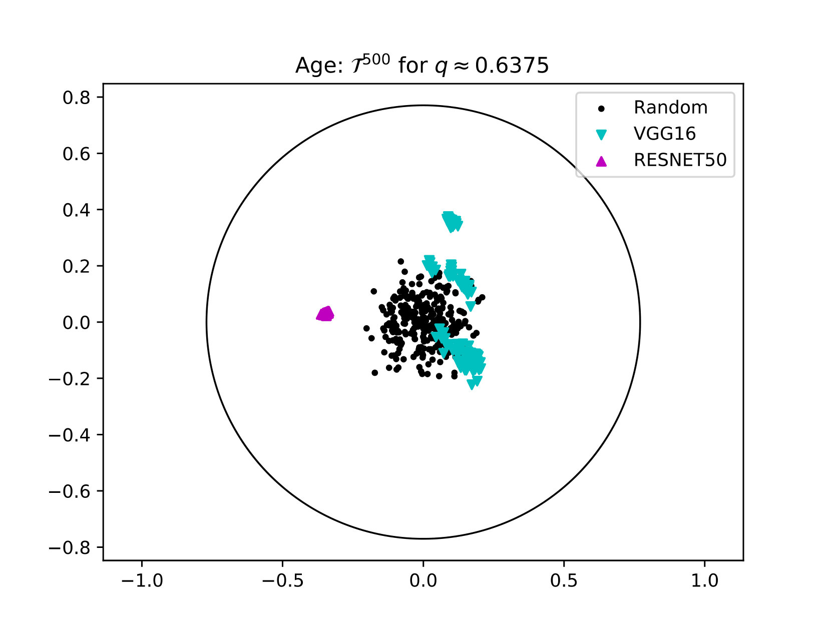 Figure 1
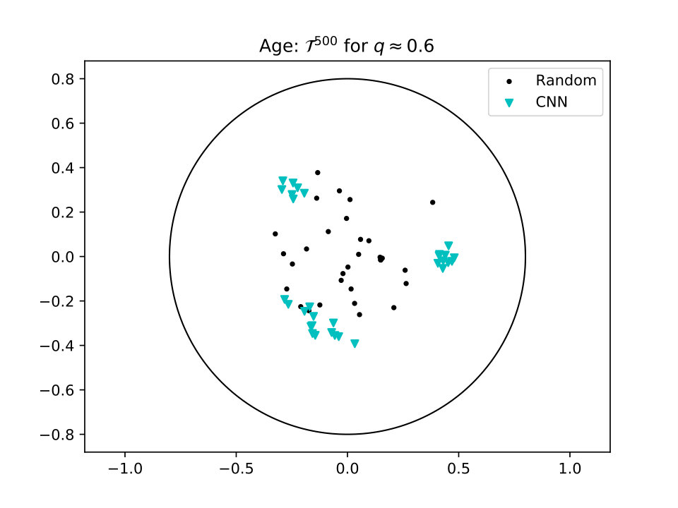 Figure 2
 Figure 3
 Figure 4
 Figure 5
 Figure 6
 Figure 7
 Figure 8
 Figure 9
 Figure 10
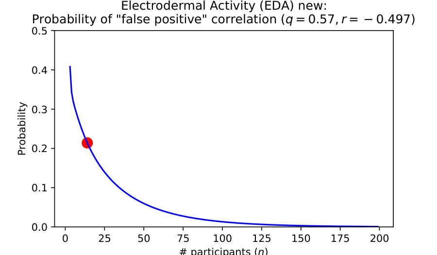 Figure 11
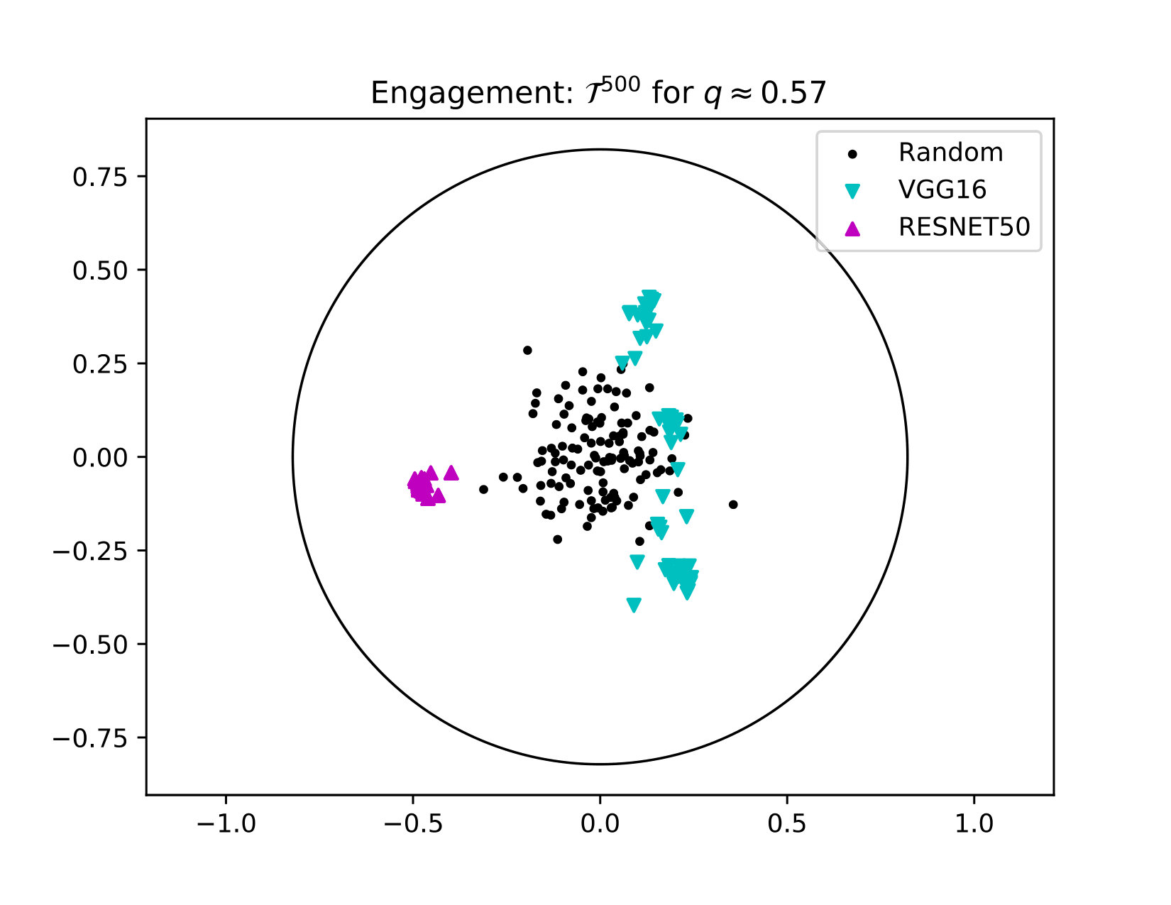 Figure 12
 Figure 13
 Figure 14
 Figure 15
 Figure 16
 Figure 17
 Figure 18
 Figure 19
 Figure 20
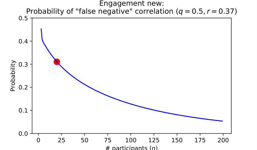 Figure 21
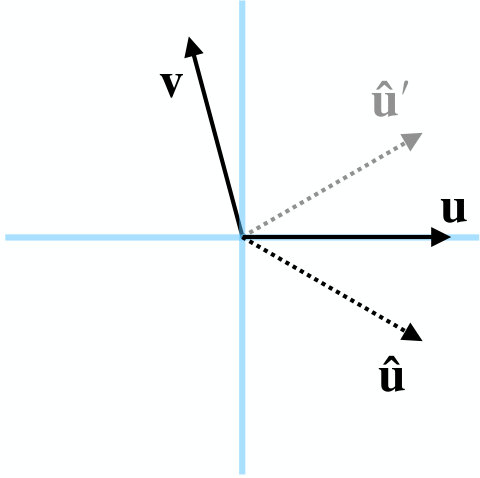 Figure 22
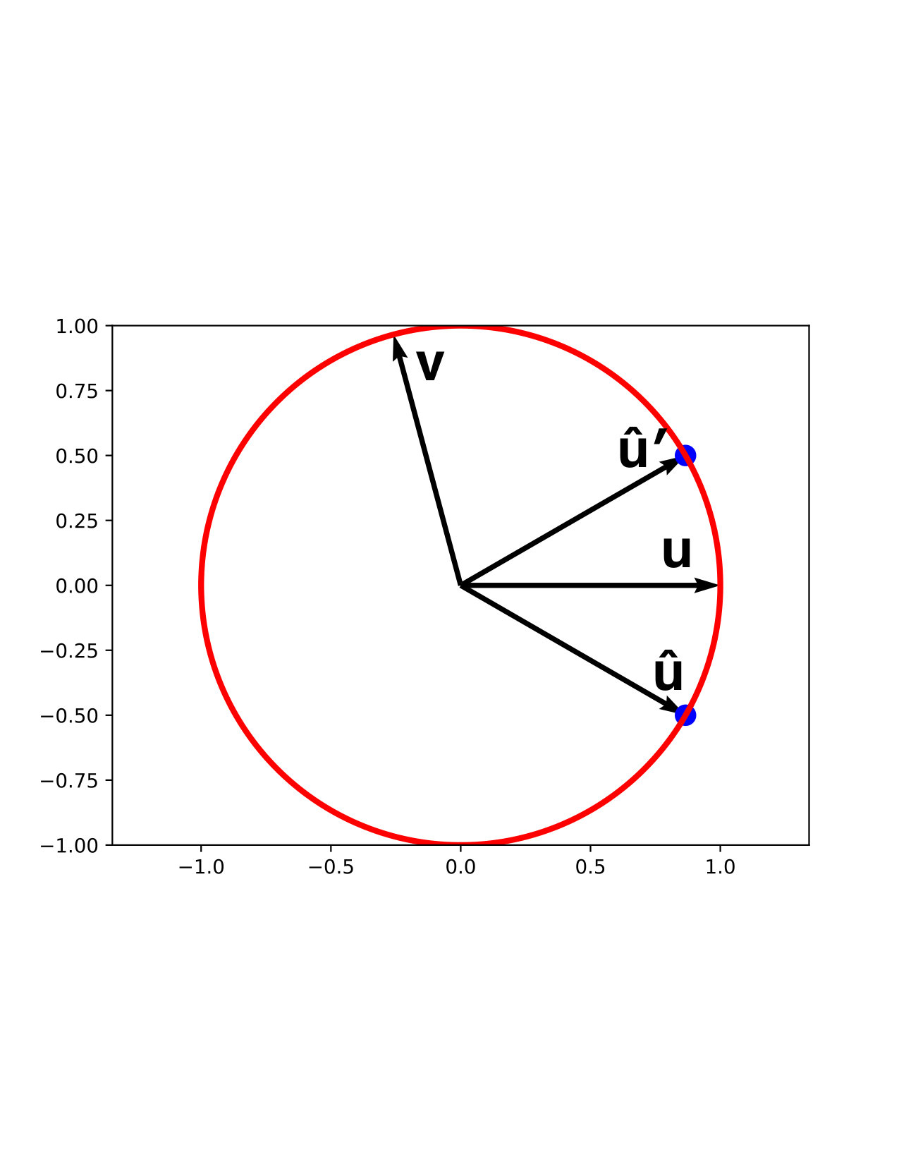 Figure 23
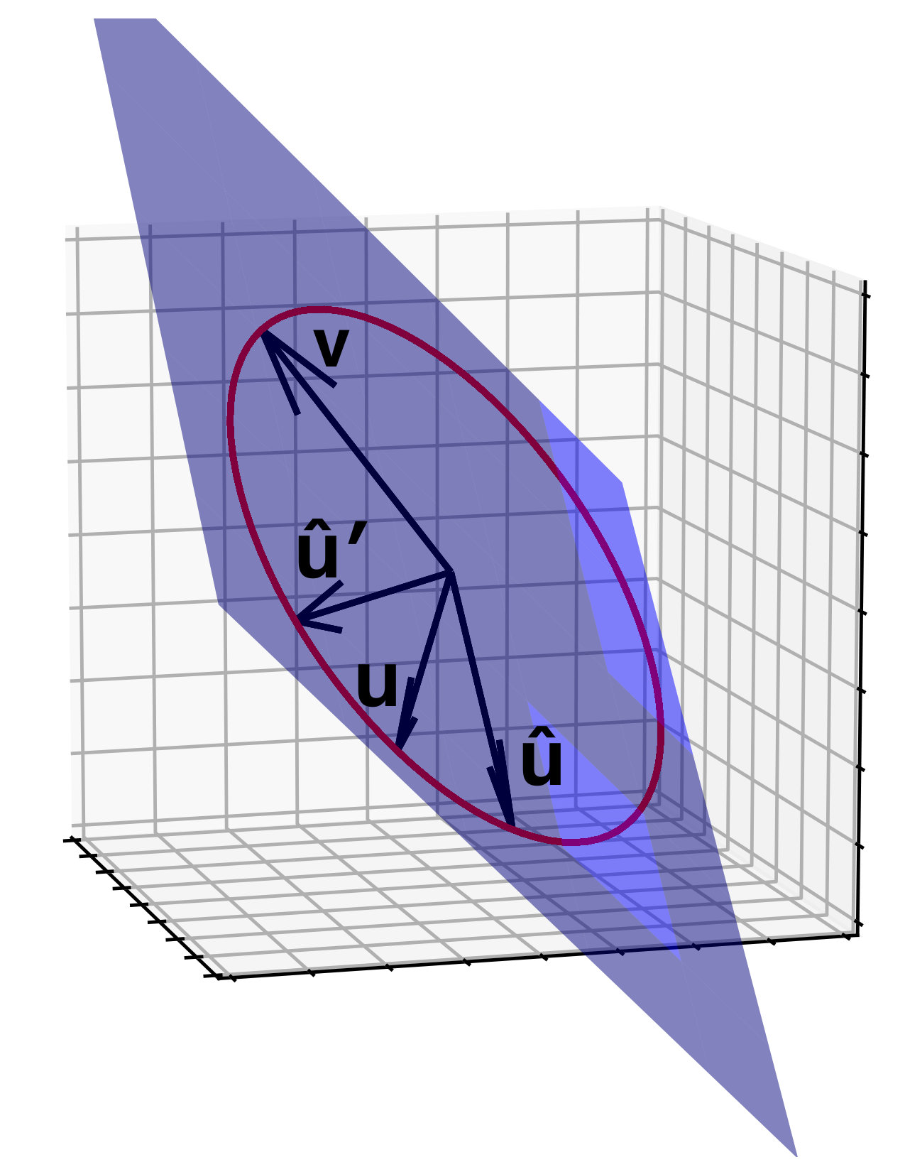 Figure 24
Peer Reviews
No public reviews on file for this paper yet. If you reviewed it on a platform where reviews are public (OpenReview, ICLR, NeurIPS, ICML), you can paste yours below so the community can read it here.
Videos
No videos yet. Explain this paper in a talk, walkthrough, or lecture? Add one.
Taxonomy
TopicsNeural Networks and Applications · Mental Health Research Topics · Anomaly Detection Techniques and Applications
Automatic Classifiers as Scientific Instruments:
One Step Further Away from Ground-Truth
Jacob Whitehill
Anand Ramakrishnan
Abstract
Automatic machine learning-based detectors of various psychological and social phenomena (e.g., emotion, stress, engagement) have great potential to advance basic science. However, when a detector is trained to approximate an existing measurement tool (e.g., a questionnaire, observation protocol), then care must be taken when interpreting measurements collected using since they are one step further removed from the underlying construct. We examine how the accuracy of , as quantified by the correlation of ’s outputs with the ground-truth construct , impacts the estimated correlation between (e.g., stress) and some other phenomenon (e.g., academic performance). In particular: (1) We show that if the true correlation between and is , then the expected sample correlation, over all vectors whose correlation with is , is . (2) We derive a formula for the probability that the sample correlation (over subjects) using is positive given that the true correlation is negative (and vice-versa); this probability can be substantial (around ) for values of and that have been used in recent affective computing studies. (3) With the goal to reduce the variance of correlations estimated by an automatic detector, we show that training multiple neural networks using different training architectures and hyperparameters for the same detection task provides only limited “coverage” of .
Pearson correlation
1 Introduction
Automatic classifiers have the potential to advance basic research in psychology, education, medicine, and many other fields by serving as scientific instruments that can measure behavioral, medical, social, and other phenomena with higher temporal resolution, lower cost, and greater consistency than is possible with traditional methods such as human-coded questionnaires or observation protocols. The affective computing (Picard, 2010) community is starting to see some first fruits of this potential: Perugia, et al. (Perugia et al., 2017) used the Empatica E4 wristband sensor to explore the relationship between participants’ () electrodermal activity (EDA) and their emotional states when playing cognitive games. Parra, et al. (Parra et al., 2017) used the Emotient facial expression recognition software to identify a positive correlation (, participants) between emotions and adult attachment (Collins & Read, 1990). Chen, et al. (Chen et al., 2014) used Emotient in a study of how facial emotion is associated with job interview performance among participants.
In most empirical studies designed to measure the relationship between two phenomena and (e.g., engagement (Monkaresi et al., 2017), grit (Duckworth et al., 2007), stress, attachment (Collins & Read, 1990), academic performance, etc.), the investigator chooses a validated instrument for each phenomenon and records measurements of each variable for participants. She/he then computes a statistic, such as the Pearson product-moment coefficient, that captures the magnitude and sign (as well as statistical significance) of the relationship between the two variables. Machine learning offers the potential to create a new array of scientific instruments with important advantages compared to standard measurement tools. However, they also bring a potential pitfall that – while not fundamentally new, i.e., there is always a separation between a construct and its measurement – is exacerbated compared to using standard measurements: If one creates a new scientific instrument by training an automatic detector to mimic a standard instrument as closely as possible, then is one degree of separation further removed from the underlying phenomenon – i.e., it is an estimator of another estimator.
Motivating example: Suppose a behavioral scientist wishes to examine the relationship between stress (construct ) and academic performance (construct ). Using a traditional approach, she/he could conduct an experiment in which each participant completes some cognitively demanding task and then takes a test. To measure stress, the scientist could also ask each participant to complete an established survey, e.g., the Dundee State Stress Questionnaire (Matthews et al., 1999). The relationship between and could then be estimated as the correlation between the vector of test scores and the corresponding vector of stress measurements over all participants.
However, suppose that the researcher also has access to an automatic stress detector that uses the participant’s face pixels to measure his/her stress level. Suppose that the accuracy of was previously validated w.r.t. a standard stress questionnaire (like (Matthews et al., 1999)), and the validation showed that the outputs of , which we denote with , have an expected correlation of with the standard questionnaire. What could go wrong, in terms of spurious deductions, when the correlation between and is estimated as instead of ?
Figure 1 shows one hypothetical example of what can go wrong: vectors contain measurements from participants of constructs and , respectively, where is obtained through a standard instrument. The Pearson product-moment correlation between two vectors can be written:
[TABLE]
where (or ) is a vector whose elements equal the mean value of (or ). Defined in this way, the value of is random if either of its two arguments is random. If and are both normalized to have 0-mean and unit-length, then their correlation depends only on the angle between them:
[TABLE]
In the figure, this correlation is , i.e., the data suggest that is negatively correlated with . Suppose instead that the researcher had used an automatic detector to obtain , where prior analysis had established that the expected correlation of ’s outputs and the standard instrument was . If the researcher uses the correlation to estimate the relationship between and , then she/he would obtain – a much larger magnitude, but at least the same sign as, the correlation obtained using a standard instrument for . But the bigger problem is the following: is not the only vector whose correlation with the “ground-truth” measurements is . Vector also has the same correlation. If the researcher obtained measurements , then she/he would deduce a positive correlation of – this is opposite to the correlation obtained with a standard instrument.
In this paper we explore how the accuracy of a scientific instrument , as measured by the Pearson correlation with the ground-truth construct , impacts the estimated correlation between constructs and . Although there are various ways of quantifying the relationship between two vectors of measurements (e.g., RMSE, MAE), the Pearson correlation is one of the most commonly used metrics. Contributions: (1) We prove that , where is the true correlation between and and random vector is sampled uniformly over the -sphere of [math]-mean unit-vectors whose correlation with is . Next, as one of the most fundamental aspects of the relationship between two variables is whether they are positively or negatively correlated, (2) we derive a function to compute the probability that the sample correlation (over subjects) using is positive, given that the true correlation between and is negative (and vice-versa). We also prove that is monotonically decreasing in and in , i.e., the danger of a false correlation is mitigated by training a more accurate detector or collecting data from more participants. Finally, (4) we explore to what extent the sphere can be “covered” by measurement vectors obtained by training different neural networks on the same dataset for the same detection task but using different configurations (e.g., architectures, hyperparameters, etc.). We also devise a novel technique to visualize this coverage of .
2 Related Work
The issue of how product-moment (Pearson) correlations among a subset of variables constrain the possible correlations among the remaining variables has interested statisticians since the 1960s. While there has been significant prior work on the trivariate case in particular, we are not aware of any work that proves exactly the same results as what we present here. (Priest, 1968) showed a lower bound on the mean intercorrelation between variables. (Glass & Collins, 1970), and also (Leung & Lam, 1975), proved that, in trivariate distributions, there are range restrictions on the possible correlations between and when the correlations between and and between and are already known. (Olkin, 1981) extended this result to multivariate distributions beyond 3 variables.
More recent, and most similar to our work, is a study by (Carlson & Herdman, 2012) from the operations research community in 2012. They examined the methodological risk of using proxy measures to estimate the correlations between different constructs. Using analytical results by (Leung & Lam, 1975), they show how the observed correlations between and can vary substantially as a function of the reliability of a proxy measure of . In contrast to our work, theirs is based on simulations and contains no formal proofs.
Finally, which vector of measurements is obtained could potentially be related to subgroup membership – e.g., gender, ethnicity, age. From the perspective of fairness in machine learning (Barocas et al., 2017; Kearns et al., 2018), it could therefore be important to understand how much variation there is among different subgroup populations over the different that are obtained from the scientific instrument.
3 Modelling assumptions
Notation: We typeset random variables in Futura font; all other variables are fixed (non-random). and are fixed -vectors of ground-truth measurements of two phenomena and , respectively. is a random -vector (sampled from ), obtained from scientific instrument , containing noisy measurements of .
For our theoretical results (Propositions 1 through 4), we assume the correlation between and is exactly ; then, is sampled uniformly from the sphere of all such vectors. However, for our empirical results regarding the probability of a “false correlation” (see Section 5), we relax this assumption: It is unlikely that instrument (that we assume was previously estimated to have correlation w.r.t. ground-truth) always produces a vector whose correlation with is exactly . Instead, the actual correlation of and comes from a sampling distribution of Pearson correlations (with “true” correlation and the number of subjects as parameters; see Section 5.1). Then, given a fixed , we sample from the corresponding (which depends on ). When we compute the probability of a “false correlation” in our case studies (Section 5.2), we marginalize over .
4 Expected Correlation of with
When we use an automatic classifier to obtain a vector of measurements, then we obtain a vector whose correlation with the underlying construct (e.g., stress) is . However, as illustrated in the example above, there can be multiple such vectors, and which one is obtained can make a big difference on the estimated correlation. As we show below, the set of [math]-mean unit-length vectors with a fixed correlation to another unit-vector is an -sphere embedded in . If we sampled uniformly at random from this sphere, then what would be the expected sample correlation between and some other vector (e.g., academic performance)?
To simplify our analyses below, we assume all have [math]-mean and unit-length since Pearson correlation is invariant to these quantities. (Regarding the uniformity assumption: see Future Work in Section 7.)
Proposition 1**.**
Let be -dimensional, [math]-mean, unit-length vectors with a Pearson product-moment correlation . Then (1) the set of [math]-mean, unit-length vectors whose correlation with is is an -sphere embedded in . Moreover, (2) if is a random vector sampled uniformly from , then the expected sample correlation .
Proof.
The set of all [math]-mean -vectors constitutes a hyperplane
[TABLE]
that passes through the origin with normal vector . The set of all unit-length vectors constitutes an -sphere
[TABLE]
embedded in . Therefore, . Figure 1 (left) shows in blue, as well as the intersection of with as a red circle. Since all three vectors have [math]-mean and unit-length, then the correlations between these vectors depend only on the angles between them. Hence, w.l.o.g. we can rotate the axes so that consists of all vectors whose first coordinate is [math], and all correlations will be preserved. After doing so, the only remaining constraint is that the projected vectors have unit-length.
More precisely, we can compute an orthonormal basis such that the first coordinate of vector is 0 for every , and such that
[TABLE]
Geometrically, this means that we can define so that the projected lie in the plane spanned by the second and third vectors in basis (see Figure 1 (right)) – this makes the rest of the derivation much simpler. represents the component of parallel to , and is the component orthogonal to . Since the correlation between and is , and since is orthonormal, then
[TABLE]
and hence . Since , then .
Now consider any vector whose correlation with is . Let us define . By construction of , we already know that . We also have
[TABLE]
and hence . Since is a unit-vector, then
[TABLE]
This set is the surface of an -sphere, with radius , embedded in . Since simply rotates the axes, then is likewise a -sphere embedded in . This proves part 1.
For part 2: When sampling uniformly from , the distribution of on the -sphere is symmetrical about 0. Then , and hence:
[TABLE]
∎
Example: For the case , consider the four vectors shown in Figure 1 (left) whose values are approximately:
[TABLE]
By construction, , and . Via a change of basis , the vectors can be rotated so that
[TABLE]
The rotated vectors are shown in Figure 1 (right). The set contains exactly two elements (since it is a [math]-sphere): and . If is sampled uniformly at random from , then . This result agrees with
[TABLE]
5 Probability of false correlations
One of the most fundamental distinctions is whether two phenomena are positively or negatively correlated with each other (or neither). What is the probability that given that the correlation (false positive correlation); or that given that the correlation (false negative correlation)? How do these probabilities change as increases or increases? The proofs of the following propositions are given in the appendix.
Proposition 2**.**
Let be the correlation between the detector’s output and ground-truth ; let be the correlation between and ; and let be sampled uniformly from . If , then the probability of a false positive correlation (in the sense defined above) is given by the function
[TABLE]
where is the 0/1 indicator function, and are the PDF and CDF of a -random variable with degrees of freedom, and . If , then the probability of a false negative correlation is also given by .
Proposition 3**.**
For every fixed and , function is monotonically decreasing in .
Proposition 4**.**
For every fixed , function is monotonically decreasing in .
Propositions 3 and 4 imply that the probability of a false correlation diminishes as increases or increases.
5.1 Marginalizing over the sampling distribution of
Up to now we have glossed over the important detail that, when a scientific instrument with average accuracy (Pearson correlation) of is used to obtain measurements for subjects, the correlation of the sampled with their ground-truth values need not be exactly ; rather, the actual correlation is drawn from a sampling distribution . Particularly for small , can deviate substantially from . Hence, to compute the probability of a false correlation, it is necessary to marginalize (via numeric integration) over :
[TABLE]
The sampling distribution of can be estimated using the formula derived by (Soper, 1913); see the appendix for more details.
5.2 Case Studies
To put these theoretical results into perspective, we conducted simulations based on two recent affective computing studies that used automated detectors as scientific instruments. The first study (), by (Perugia et al., 2017), used an Empatica E4 wrist sensor to investigate how electrodermal activity (EDA) () is correlated with the subjects’ emotions (). The second study (), by (Whitehill et al., 2014), explored the relationship between student engagement (), as measured by an engagement detector that analyzes static images of students’ faces, and test performance () in a cognitive skills training task. In order to estimate the probability of a false correlation (in the sense described above), we need to know the accuracy of the automatic detector – i.e., the correlation between the automatic measurements and ground-truth of construct – as well as the true correlation between constructs and .
Estimating and : The value of can easily be estimated using cross-validation or other standard procedures. For the first study (EDA), we use the value reported in (Poh et al., 2010) for cognitive tasks with a distill forearm sensor of EDA. The value of is not knowable without access to ground-truth measurements; instead, we hypothesize that the ground-truth correlation between and is exactly what was estimated by the authors (Perugia et al., 2017) using the E4 sensor and emotion survey instruments: . For the second study (Engagement), we use the value reported in (Whitehill et al., 2014) that was obtained using subject-independent cross-validation. For , we use the correlation obtained by the authors () when correlating test performance with human-labeled student engagement.
Results: Plots of the probability of a false correlation (obtained from function derived above) as a function of the number of participants are shown for each study (with their associated and values) in Figure 2. The red dot in each graph shows the actual number of participants from each experiment. Even for subjects, the probability is non-trivial. For the values and , these probabilities are substantial – around for the EDA study and around for the Engagement study. The possibility of a false correlation is not protected against by statistical significance testing – it is possible for the estimated correlation between constructs and to be highly significant and yet have the wrong sign compared to the ground-truth correlation. While this is almost always theoretically possible due to the inherent separation between a construct and its measurement, the use in basic research of automatic detectors that are trained to estimate another estimator can make this problem worse.
6 Coverage of when training a detector
Given that which vector is obtained from an automatic detector can substantially impact the estimated correlation between constructs and , it could be useful to average the sample correlations over many vectors from , i.e., to compute . This could help to reduce the variance of the estimator. In this section we explore whether it is feasible to generate many different , all with similar correlation with ground-truth , by training a set of automatic detectors using slightly different training configurations. In particular, we varied: (1) the architecture (VGG-16 (Simonyan & Zisserman, 2014) versus ResNet-50 (He et al., 2016)) and (2) the random seed of weight initialization. Inspired by recent work by Huang, et al. (Huang et al., 2017) on how an entire ensemble of detectors can be created during a single training run, we also varied (3) the number of training epochs, and saved snapshots of the trained detectors at regular intervals.
During training, each detector’s estimates of the test labels evolves, and so does the correlation between and the ground-truth labels . However, for the tasks we examined (described below), the test correlations tend to stabilize over time, and they converge to roughly the same value even across different training runs and detection architectures. Given a set of measurement vectors (produced by detectors ) whose accuracies (Pearson correlations with ground-truth) are all approximately , we can project them onto the -sphere of [math]-mean, unit-length vectors whose correlation with is . We can then visualize the “coverage” of this sphere by projecting it onto a 2-D plane, and also compare the coverage to a random sample of elements of .
We explored the coverage of for two automatic face analysis problems: student engagement recognition and age estimation using the HBCU (Whitehill et al., 2014) (Engagement) and GENKI (Lab, ) (Age) datasets, respectively; see Figure 3 for labeled examples.
6.1 Detection architectures
We examined two modern deep learning-based visual recognition architectures – VGG-16 (Simonyan & Zisserman, 2014) and ResNet-50 (He et al., 2016) – to assess how much “coverage” of each architecture can produce, as well as to compare the variability of the resulting measurement vectors to each other.
6.2 Training procedures
Engagement detector: We performed training runs for each of the two network architectures (VGG-16, ResNet-50). Training data consisted of face images from 15 subjects of HBCU (Whitehill et al., 2014), and testing data were images from the remaining 5 subjects. (This corresponds to just one cross-validation fold from the original study (Whitehill et al., 2014).) Optimization was performed using SGD for iterations, and the network weights were saved every iterations. In total, this produced detectors. The average correlation (over all detectors) between the detectors’ test outputs and ground-truth was (s.d. ) for VGG-16 and (s.d. ) for ResNet-50. Inspired by (Huang et al., 2017), we also tried both cosine and triangular (Smith, 2017) learning rates. However, in pilot testing we found that these delivered worse accuracy than exponential learning rate decay and we abandoned the approach.
Age detector: We performed training runs for VGG-16 and ResNet-50 using SGD for with snapshots every iterations, as for engagement recognition. This produced detectors. Training data consisted of face images of the GENKI dataset (Lab, ), and testing data consisted of face images. The average correlation of the automatic measurements with ground-truth on the test set was (s.d. ) for VGG-16 and (s.d. ) for ResNet-50.
6.3 Visualizing elements of the -sphere
Given a set of trained detectors, we can sample vectors of age/engagement estimates whose correlation with ground-truth is approximately . Then we can visualize how these vectors “cover” the -sphere using the following procedure:
Normalize , as well as each , to have [math]-mean and unit-length. 2. 2.
Compute an orthonormal basis (e.g., using a QR decomposition) so that (a) the first component of is [math] for every , and (b) (see Equation 1). 3. 3.
Project each onto the new basis . By construction, the first component of each projection will be [math] and the second component will be . 4. 4.
Define each to be the last components of vector . 5. 5.
Project the onto the two principal axes obtained from principal component analysis (PCA).
Since the 2-D projection of a 0-centered sphere onto any orthonormal projection is a disc, the output of the procedure above is a set of points that lie on a disc of radius .
6.4 Generating random vectors on
In order to assess how evenly the sphere is “covered” by the vectors obtained from the automatic detectors, we can generate random vectors of and likewise project them onto a 2-D disc. We generate each such vector as follows:
Sample each () from a standard normal distribution. 2. 2.
For , set .
We then project the vectors in the set onto the two principal axes obtained from PCA. To enable a fair comparison between the variances of the randomly generated elements of and those obtained from the trained detectors, we run PCA separately for each set.
6.5 Results
We projected all vectors whose correlation with was between and for Engagement recognition and and and Age estimation; this amounted to of the engagement detectors and of the age detectors. The projections are shown for each task in Figure 4. First, we observe that there is some “spread” – the measurement vectors occupy different clusters on the sphere. This indicates that the same training data can still yield automatic measurements on testing data whose correlations with each other is far less than 1. In fact, for engagement recognition, the minimum correlation, over all pairs , was .
For engagement recognition, the VGG-16 based measurements and the ResNet-50 based measurements each resided within their own clusters on the sphere, and these clusters did not overlap. This suggests that, even though both architectures yielded similar overall accuracies, they are making different kinds of estimation errors on the test set. Interestingly for both age estimation and engagement recognition we can see that VGG-16 has a bigger “spread” compared to ResNet-50. We speculate this might be due to VGG-16 ( million) having significantly more parameters compared to ResNet-50 ( million), thus enabling it to learn more varied features.
Finally, a comparison of the variance between the automatic measurements and random samples from indicates that varying the training configuration (architecture, hyperparameters) provides only limited ability to cover the sphere: the variance in the vectors, as quantified as the sum of the trace of their covariance matrix, was statistically significantly less compared to randomly sampled points on (, 1-tailed, Monte Carlo simulation).
7 Conclusions
Advances in machine perception present a powerful opportunity to create new scientific instruments that can benefit basic research in sociobehavioral sciences. However, since detectors are often trained to estimate existing measures, which are already only an estimate of underlying constructs, then these instruments are essentially one step further removed from ground-truth. For this reason, it is important to interpret results obtained with them with care.
In this paper, we investigated how measurements of construct obtained with an automatic detector can impact the estimated correlation between and another construct . We showed that: (1) The set of [math]-mean unit-length -vectors with a fixed Pearson product-moment correlation to vector is a -sphere embedded in . (2) If the correlation between automatic measurements and the ground-truth measurements is ; if the true correlation between and is ; and if is sampled uniformly from ; then the expected sample correlation obtained with the automatic detector is . (3) The probability of a “false correlation”, i.e., a sample correlation between constructs and whose sign differs from the true correlation, is monotonically decreasing in (number of participants) and also monotonically decreasing in (accuracy of the detector). These probabilities can be non-trivial for small values of that are nonetheless sometimes found in contemporary research using automatic facial expression and affect detectors. Moreover, the danger of a false correlation is not eliminated through statistical significance testing. (4) We explored empirically how efficiently multiple neural network-based detectors of age and student engagement, when trained using different architectures and hyperparameters but the same training data, can “cover” the sphere .
In practice, our results suggest that, particularly when the number of participants is small and/or the accuracy of the detector is modest, it is important to consider the possibility of a false correlation, or at least a skewed correlation (by factor ), when drawing scientific conclusions.
Limitation and future work: In our study we assumed that is a random sample from the uniform distribution over – this expresses the idea that a priori we may have no idea which particular element of detector will return. In reality, however, detectors have biases – e.g., due to head pose, lighting conditions, training set composition, etc. – and these can affect which element of is obtained.
Acknowledgements: This research was supported by a Cyberlearning grant from the National Science Foundation (grant no. #1822768).
8 Appendix
8.1 Proof of Proposition 2
We prove the proposition for the case that ; the case for is similar.
From Section III, we have that
[TABLE]
Since each () is a coordinate on an -sphere, it can be re-parameterized (Muller, 1959) by sampling standard normal random variables and normalizing, i.e.:
[TABLE]
where each . A false positive correlation thus occurs when is at least more than its expected value :
[TABLE]
Due to the inequality, we must handle the cases that and separately. Note that the latter case contributes 0 probability since and . Also, since is a standard normal random variable, .
[TABLE]
For , each side of the inequality is a sum of squared normally distributed random variables, i.e., a -random variable (though with different degrees of freedom). We can thus rewrite this probability as
[TABLE]
where and are random variables with and degrees of freedom, respectively. The probability is equivalent to the integral because, for any value of the variable, we require that the variable be less than (after applying a scaling factor). To our knowledge, there is no closed formula for this integral, but we can compute it numerically. For , we have
[TABLE]
since a -random variable is non-negative, and where the probability of is if the inequality is true and [math] otherwise.
8.2 Proof of Proposition 3
For convenience, define .
[TABLE]
Ghosh (Ghosh, 1973) proved that, for any fixed , is monotonically increasing in the degrees of freedom ; hence, is monotonically decreasing in . Therefore, for all . Since is a non-negative function for all , then the integral in Equation 8.2 must be negative; hence, is monotonically decreasing in for every and .
8.3 Proof of Proposition 4
First, we show that is monotonically decreasing in :
[TABLE]
The first term is monotonically decreasing in , and the second term is constant in .
Next, let be a positive real number such that :
[TABLE]
Since is monotonically increasing, then the expression in brackets is negative. Since is non-negative, then the entire integral must be less than 0.
9 Sampling distribution
The sampling distribution can be computed exactly (Fisher, 1915), but this is computationally feasible only for small . Hence, we use the approximation from Soper (Soper, 1913): Let denote the population Pearson correlation coefficient, and let denote the sample correlation from data. Then
[TABLE]
The reference list from the paper itself. Each links out to its DOI / PubMed record.
- 1Barocas et al. (2017) Barocas, S., Hardt, M., and Narayanan, A. Fairness in machine learning. In Conference on Neural Information Processing Systems, Long Beach, CA , 2017.
- 2Carlson & Herdman (2012) Carlson, K. D. and Herdman, A. O. Understanding the impact of convergent validity on research results. Organizational Research Methods , 15(1):17–32, 2012.
- 3Chen et al. (2014) Chen, L., Yoon, S.-Y., Leong, C. W., Martin, M., and Ma, M. An initial analysis of structured video interviews by using multimodal emotion detection. In Proceedings of the 2014 workshop on Emotion Representation and Modelling in Human-Computer-Interaction-Systems , pp. 1–6. ACM, 2014.
- 4Collins & Read (1990) Collins, N. L. and Read, S. J. Adult attachment, working models, and relationship quality in dating couples. Journal of personality and social psychology , 58(4):644, 1990.
- 5Duckworth et al. (2007) Duckworth, A. L., Peterson, C., Matthews, M. D., and Kelly, D. R. Grit: perseverance and passion for long-term goals. Journal of personality and social psychology , 92(6):1087, 2007.
- 6Fisher (1915) Fisher, R. A. Frequency distribution of the values of the correlation coefficient in samples from an indefinitely large population. Biometrika , 10(4):507–521, 1915.
- 7Ghosh (1973) Ghosh, B. Some monotonicity theorems for χ 2 superscript 𝜒 2 \chi^{2} , F 𝐹 {F} and t 𝑡 t distributions with applications. Journal of the Royal Statistical Society. Series B (Methodological) , pp. 480–492, 1973.
- 8Glass & Collins (1970) Glass, G. V. and Collins, J. R. Geometric proof of the restriction on the possible values of rxy when r xz and ryz are fixed. Educational and Psychological Measurement , 30(1):37–39, 1970.