Strong Convexity for Risk-Averse Two-Stage Models with Fixed Complete Linear Recourse
Matthias Claus, Kai Sp\"urkel

TL;DR
This paper extends the understanding of strong convexity in two-stage risk-averse models with linear recourse, providing conditions for various risk measures and implications for stability and optimization algorithms.
Contribution
It introduces the concept of partial strong convexity and derives verifiable conditions for strong convexity in models with distortion risk measures.
Findings
Conditions for strong convexity in models with CVaR and distortion risk measures.
Implications for stability under probability measure perturbations.
Relevance for convergence rates in stochastic optimization algorithms.
Abstract
This paper generalizes results concerning strong convexity of two-stage mean-risk models with linear recourse to distortion risk measures. Introducing the concept of (restricted) partial strong convexity, we conduct an in-depth analysis of the expected excess functional with respect to the decision variable and the threshold parameter. These results allow to derive sufficient conditions for strong convexity of models building on the conditional value-at-risk due to its variational representation. Via Kusuoka representation these carry over to comonotonic and distortion risk measures, where we obtain verifiable conditions in terms of the distortion function. For stochastic optimisation models, we point out implications for quantitative stability with respect to perturbations of the underlying probability measure. Recent work in \cite{Ba14} and \cite{WaXi17} also gives testimony to the…
Click any figure to enlarge with its caption.
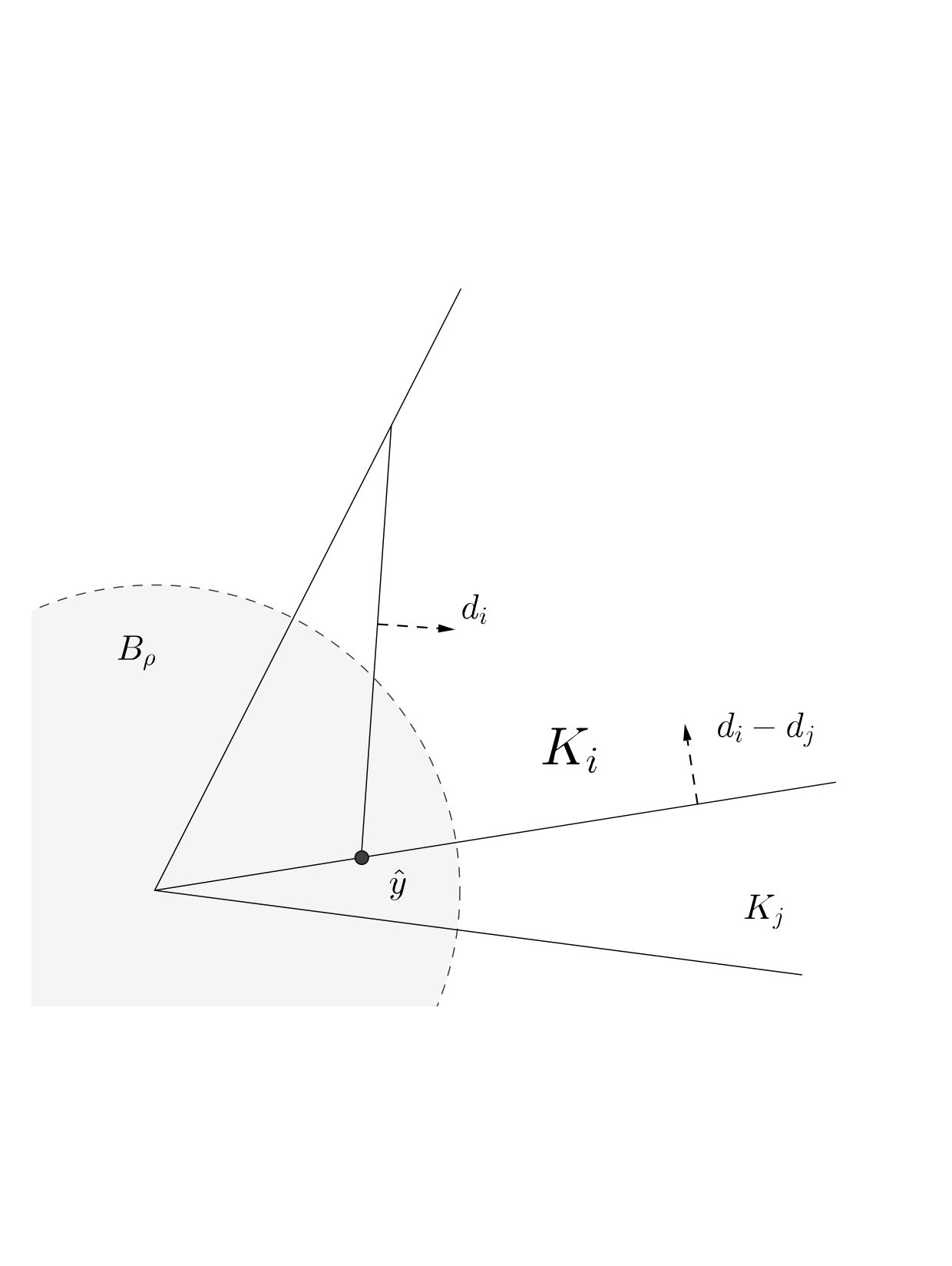 Figure 1
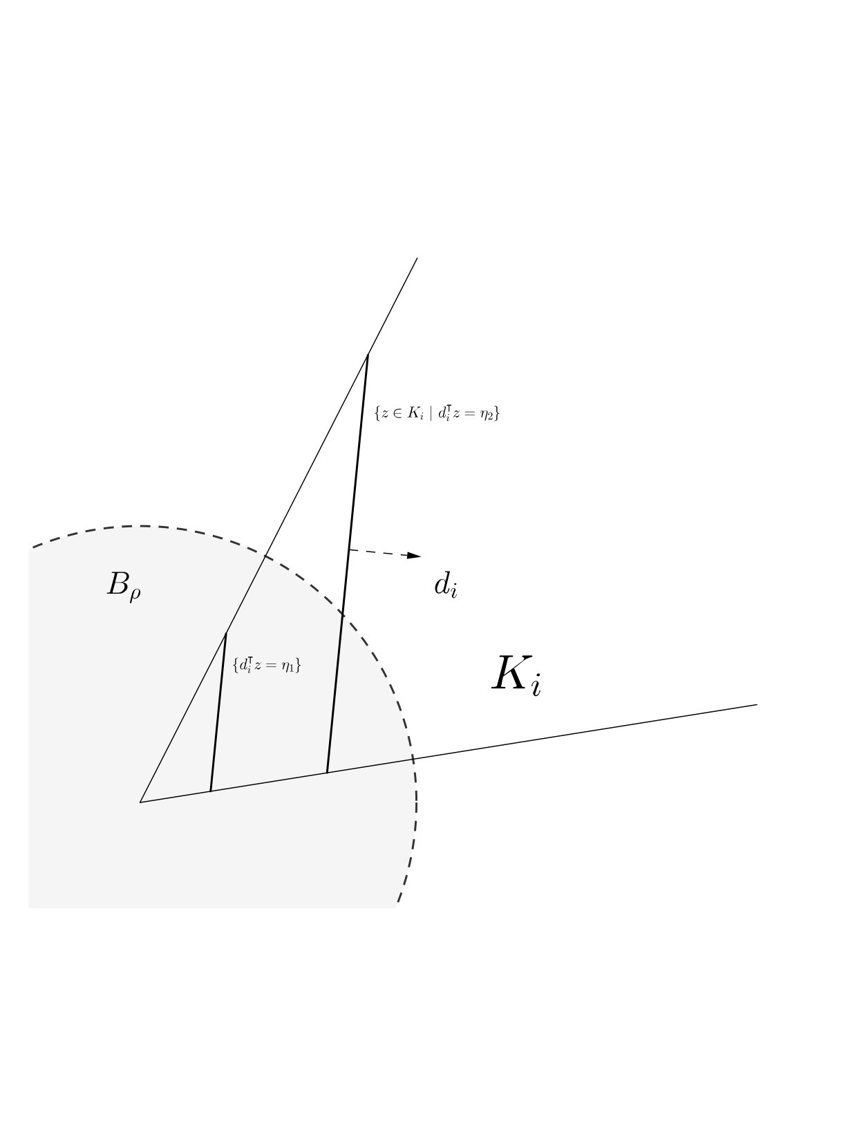 Figure 2
Peer Reviews
No public reviews on file for this paper yet. If you reviewed it on a platform where reviews are public (OpenReview, ICLR, NeurIPS, ICML), you can paste yours below so the community can read it here.
Videos
No videos yet. Explain this paper in a talk, walkthrough, or lecture? Add one.
Taxonomy
TopicsRisk and Portfolio Optimization · Statistical Methods and Inference · Stochastic processes and financial applications
∎
11institutetext: M. Claus 22institutetext: University Duisburg-Essen
Thea-Leymann-Straße 9
D-45127 Essen
Tel.: +49 201 183 6887
22email: [email protected] 33institutetext: K. Spürkel 44institutetext: University Duisburg-Essen
Thea-Leymann-Straße 9
D-45127 Essen
Tel.: +49 201 183 6890
44email: [email protected]
Strong Convexity for Risk-Averse Two-Stage Models with Fixed Complete Linear Recourse
††thanks: The authors gratefully acknowledge the support of the German Research Foundation (DFG) within the collaborative research center TRR 154 “Mathematical Modeling, Simulation and Optimization Using the Example of Gas Networks”.
Matthias Claus
Kai Spürkel
(Received: date / Accepted: date)
Abstract
This paper generalizes results concerning strong convexity of two-stage mean-risk models with linear recourse to distortion risk measures. Introducing the concept of (restricted) partial strong convexity, we conduct an in-depth analysis of the expected excess functional with respect to the decision variable and the threshold parameter. These results allow to derive sufficient conditions for strong convexity of models building on the conditional value-at-risk due to its variational representation. Via Kusuoka representation these carry over to comonotonic and distortion risk measures, where we obtain verifiable conditions in terms of the distortion function. For stochastic optimisation models, we point out implications for quantitative stability with respect to perturbations of the underlying probability measure. Recent work in Ba14 and WaXi17 also gives testimony to the importance of strong convexity for the convergence rates of modern stochastic subgradient descent algorithms and in the setting of machine learning.
Keywords:
Two-Stage Stochastic Programming Linear Recourse Strong Convexity Conditional Value at Risk Comonotonic Risk Measures Stability
MSC:
90C15 90C31
1 Introduction
In S94 Schultz considered the expectation based two-stage optimisation problem
[TABLE]
where is a subset of some , convex and real-valued, a -dimensional random vector on some propability space and a recourse function of the form
[TABLE]
which is the value function of a linear program with parametric right-hand side. For a general introduction to such models we refer to the standard textbooks BL11 and SDR14 . The optimisation problem (1) can be rewritten as
[TABLE]
with
[TABLE]
and the reduced expectation function
[TABLE]
where denotes the pushforward measure of . It is well-known that under mild assumptions is well-defined and convex on all of . For further structural analysis of the optimisation problem (1) (e.g. stability analysis, cf. section 4) and its algorithmic treatment with subgradient schemes (cf. Nes04 ) conditions for strong convexity may be desirable and for the risk-neutral setting were given in S94 , Theorem 2.2:
Theorem 1.1
Assume that the following conditions are satisfied:
- A1
For every there exist some such that . (Complete recourse)
- A2
There exists some with . (Strengthened sufficiently expensive recourse)
- A3
* is -integrable. (Finite first moments)*
- A4
* has a density with respect to the Lebesgue-measure and there exists a convex open set , constants such that a.s. on .*
Then is strongly convex on .
Remember that a real-valued function on some convex subset of a normed space is called -strongly convex on that set if for all and all it holds
[TABLE]
We point out that a constant of strong convexity for in Theorem 1.1 can be computed from the model data, i.e. the geometry of the set , and .
In CSS17 the analysis of (5) was extended to the upper semideviation based functional
[TABLE]
and the expected-excess based one
[TABLE]
which, for simplicity, we shall call upper semideviation and expected excess repectively. For the latter one an additional assumption A5 on the magnitude of is needed because if is too big, might not even depend on anymore.
1.1 On strong convexity of for fixed
In order to formulate condition A5 we note the following properties of the value function and its linearity complex (cf. Lemma 32 and 34 in CSS17 ):
Lemma 1
Assume A1 and A2. Then is the convex hull of its finitely many extreme points and has the following properties:
- (i)
, for all , i.e. is finite and polyhedral.
- (ii)
* with each being a -dimensional, pointed polyhdral cone. Furthermore each with is a common closed face of and and it holds if and only if and are adjacent.*
- (iii)
There is some such that
[TABLE]
Let us fix some more notation:
Since each is a polyhedral cone, we can write it as the conic hull of its finitely many extreme-rays, i.e. . With shorthand and we note that for and it holds that the hyperplane intersects at least one extreme ray of in a single point:
[TABLE]
for at least one . Let denote one with minimum norm. Theorem 35 in CSS17 can then be formulated as this:
Theorem 1.2
Let A1-A4 hold. In addition assume
- A5
* is such that for all we have (where is the one given in A4).*
Then is strongly convex on (cf. A4 for the definition of ) with respect to for all . The modulus of strong convexity does not depend on .
The geometric situation is shown in Fig. 1.
In A5 it is in fact enough to show that for every it holds or if there exist an index set such that it holds for all . In this paper we shall use the slightly less general version of A5.
Let us make three remarks on the theorem:
Firstly, it is desirable to verify condition A5 for as large as possible (especially when considering Theorem 2.3 later). The larger and with , the larger can be chosen.
Secondly, condition A5 might not be fulfilled on the entire set . By considering a subset instead, allowing for a possibly bigger value of , one can ensure that condition A5 holds on at least. Hence, strong convexity of can be shown on a smaller set. We shall demonstrate these two remarks in Example 1 below.
Thirdly, a modulus of strong convexity can be computed in terms of model-data directly with the techniques employed in CSS17 . It depends on , the shape of , the lower bound of ’s density and (all subsumized as ”model data”). There is a certain trade-off between how big can be and how is chosen: The bigger , the smaller . Example 2 illustrates this fact.
In Theorem 2.3 and Theorem 2.4 we will calculate moduli of strong convexity for in a more general setting than in Theorem 1.2.
Example 1
Consider and . For arbitrary we compute for
[TABLE]
We see that is strongly convex as long as the condition is fulfilled. In notation of A5 there is only one cone with which is corresponding to . We get and condition A5 reads so that is strongly convex on whenever . If we may consider the set to get strong convexity for larger than before. We can set as the new and see that is strongly convex on for all .
Note that the modulus of strong convexity does not depend on or which in higher dimensional cases cannot be expected:
Example 2
Let , .
We shall also assume , and when computing
[TABLE]
For the tedious computation we refer to the appendix. The components of the Hessian of are
[TABLE]
If , we can choose close to and close to [math] which gives . Since the determinant of the Hessian is equal to the product of its Eigenvalues we see that at least one of them approaches [math] so that the modulus of strong convexity must depend on the choice of given in condition A5.
1.2 Variational representation of CVaR
In section 3 we shall consider the Conditional Value-at-Risk at a confidence level , which can be characterized by a minimisation problem in terms of :
[TABLE]
For smooth distributions this representation is due to (UR99, , Theorem 1), while (UR02, , Theorem 10) covers the general case and shows that the Value-at-Risk
[TABLE]
is an optimal solution to the above minimisation problem. Thus,
[TABLE]
We shall however favor working with representation (6) due to inconvenient properties of , i.e. absence of convexity. While it is straightforward to show convexity of through (6) essentially due to joint convexity of in both arguments, strong convexity does not follow trivially even if is strongly convex in with strong convexity constant not depending on . A property that ensures strong convexity of can be defined as follows:
Definition 1
Let and nonempty and convex.
A function is called partially -strongly convex with respect to its first argument if
[TABLE]
holds for all .
Lemma 2
If (as above) is continuously differentiable then partial strong convexity is equivalent to
[TABLE]
for all .
Although the proof is virtually the same as for strong convexity (cf. RhOr70 ) in both arguments, we shall give a variant of the proof in for the reader’s convenience in the appendix.
For the moment let us assume that is partially strongly convex with respect to on some set . The following simple calculation shows that is strongly convex on with modulus if .
For any and set , . Then
[TABLE]
where the second inequality follows from being partially strongly convex.
One might hope that conditions A1-A5 suffice to prove partial strong convexity for . It turns out, that this is not true:
Example 3
As a counterexample consider
[TABLE]
with and (i.e. uniformly distributed on . Let so that conditions are satisfied. Also choose so that A5 holds. In case we get
[TABLE]
We calculate for
[TABLE]
as long as . Since for small we can choose , cannot be partially strongly convex in wrt. on the set .
In this example does not have the desired joint convexity properties on any open set contained in the support of .
Unsurprisingly, does not behave any better:
Example 4
With the same specifications as in example 3 we can calculate the conditional value at risk at some level for any as (cf. (6))
[TABLE]
The unique minimizer is . Note that we can restrict the minimisation to since the value at risk is obviously positive. We arrive at
[TABLE]
so there is no subset on which is strongly convex.
We shall give a rather strict condition on the value function that yields partial strong convexity for the expected excess in section 3 without additional assumptions on the distribution of .
Before that we will introduce the even weaker concept of strong convexity, restricted partial strong convexity, which can be shown to hold for under less restrictive assumptions on the recourse function. This property can also be characterized by monotonicity of the gradient as in Lemma 2.
Definition 2
Let and nonempty and convex.
A function is called restricted partially -strongly convex on with respect to its first argument if
[TABLE]
for all and all .
Note that does not need to be a cylindrical subset of as in Definition 1.
In section 3 we will show that conditions A1-A5 are sufficient for restricted partial strong convexity of on some nonempt set . The estimates above showing that partial strong convexity of implies strong convexity of can be used verbatim to show that restricted partial strong convexity of does so as well - if one can additionally show that for all (or maybe for all ). Example 4 shows that this cannot be done without only relying on assumptions A3 and A4 on the distribution of .
2 Joint properties of
Theorem 1.2 addresses properties of for fixed threshold . In Theorem 2.3 we will show that in conjunction with A1-A5 the following condition is sufficient for partial strong convexity of wrt. :
- A6
It holds , i.e. the gradient of the objective function of the second stage is positive componentwise (cf. (2)).
Note that this condition is stronger than A2 (choose there). Although it is a rather strict condition on the problem data, it might be well justifiable in the setting of simple recourse problems because compensating actions in the second stage should have negative impact on the total objective.
If A6 does not hold, all that can be shown is restricted partial strong convexity in the sense of Definition 2. We start with an elementary lemma to provide some geometrical insights that are used within the proof of Theorems 2.3 and 2.4:
Lemma 2.1
Let A1 and A2 hold. Then A6 is fulfilled if and only if one of the following conditions is fulfilled:
- (i)
There is some such that for all it holds
[TABLE]
- (ii)
For all we have .
Proof
This follows directly from well-known separating hyperplane theorems.
Lemma 2.2
Let A1-A4 hold. Then is continuously differentiable and we have the following formula:
[TABLE]
with suitable parametric sets sets to be constructed in the proof below.
Proof
By assumptions A1-A4 and standard arguments is continuously differentiable on , so only (2.2) warrants a proof. We calculate
[TABLE]
with shorthand .
Let and
[TABLE]
Define random variables and taking values with probability and with probability respectively. We observe that the quantities in (2) can be rewritten as Riemann-Stieltjes integrals with cdfs as integrators:
[TABLE]
Integration by parts yields
[TABLE]
Note that the boundary terms cancel out because for all .
Introducing the index set
[TABLE]
and observing that the sets only meet in lower dimensional sets (if they meet at all) and thus for , we can write down the cdfs and as follows:
[TABLE]
Note that can be written as the measure of a difference of sets if we can show that the following inclusion holds for all :
[TABLE]
First note that for all we have
[TABLE]
for if it was not true there would be some contained in the union to the left side of the inclusion but not in the right. This means there is some index with such that . Since the cones cover the entire space (cf. Lemma 1 (ii) ) there is some index such that and . By using the definition of the sets we arrive at the contradiction
[TABLE]
Back to (14) we see that this inclusion reduces to (15) in case which was just discussed. Now let and for some which implies , and . This yields
[TABLE]
Since by (15) we also have for some we have shown that and (14) is proven. We can now replace and conclude the proof with
[TABLE]
∎
Since is continuously differentiable we can prove (restricted) partial strong convexity of by showing that (9) (and its restricted counterpart) holds for , i.e. showing that there exists some with
[TABLE]
for relevant .
This is done by restricting the area of integration in (2.2) to some subset with measure not smaller than for some constant . Then the -measure of the set within the integrand will be estimated from below by constructing a cylindrical subset with Lebesgue measure not smaller than (with some other constant ) and which is contained in , where a lower bound on ’s Lebesgue-density is available. We begin with the special case employing condition A6:
Theorem 2.3** (Partial strong convexity of )**
*Let A1-A6 hold.
Then is partially strongly convex on the set wrt. .*
Proof
Crucially relying on A6 we may assume , otherwise substitute and and consider and instead of and . Since the sets cover the entire space we can pick an index such that . Note that in condition A5 and the discussion before it, which will come into play soon, we have and for all indices .
We shall now construct some and give the desired estimate of (2.2) for first. By Lemma 1 (iii) there is some index different from such that
[TABLE]
Assume that . This implies and is implied by for all with . We thus find the inclusion
[TABLE]
where the set on the right-hand side does not depend on anymore. We want to estimate the -measure of this set:
Remember that is a pointed cone and therefore has finitely many facets and finitely many extreme-rays adjacent to facet . For notational convenience set
[TABLE]
Intersecting with a hyperplane - this really is a hyperplane since - yields points where the hyperplane meets the extreme rays of adjacent to :
[TABLE]
Among all pick some with
[TABLE]
Choose such that
[TABLE]
which is possible since as , and let .
For all we can now show the inclusions
[TABLE]
To this end let with and be given. It holds due to the convexity of . Furthermore
[TABLE]
It remains to be shown
[TABLE]
Due to and we have , since is a convex cone. We also have
[TABLE]
which establishes . Let be any index in such that . We will show that does not even lie in :
[TABLE]
where we used the fact that , implying , and .
As the last prerequisite step we want to show that there exists some constant such that
[TABLE]
First note that we may as well set due to the translation invariance of the Lebesgue measure. The set is then the Lebesgue measure of a cylindrical set with bases and .
Let
[TABLE]
This constant still depends on the index which in turn depends on the direction . Since there are only finitely many possible choices of we can robustify by picking the minimal .
The estimate (23) then follows from (17) and Cavalieri’s principle. As a side-remark - which comes into play when trying to maximize the constant of partial strong convexity - we note that the function
[TABLE]
is continuous, monotonically decreasing and tends to \lambda_{s-1}\big{(}F^{i}_{j}\cap B_{\rho}(0)\big{)} as .
We have gathered all necessary information to continue in (2.2) as
[TABLE]
In the first inequality the nonnegativity of the integrand and in the only equality the translation invariance of the Lebesgue measure was used.
Choose now some with
[TABLE]
and set
[TABLE]
Now consider the case :
We will choose as the area of integration in (2.2). As the integration variable satisfies we can find a subset of the one in (2.2) as
[TABLE]
In analogy with the notation used in the previous case set
[TABLE]
It holds
[TABLE]
Inclusion (27) follows the same way as (21). The proof for (28) works similar to the one for (22) with minor modifications:
Let with and . Again due to being a convex cone. Furthermore
[TABLE]
because and . Thus has been established. Pick any index with . It holds
[TABLE]
so we have . In the last inequality we have used .
As the last ingredient we will show that there exist constants
[TABLE]
To this end set
[TABLE]
which is positive by construction. Applying Lemma 2.1 (i) and Cavalier’s principle yields (29). Having a lower bound on the measure of the set is the reason why we need to have to distinct the cases and in the first place.
With this we can continue (2.2) as
[TABLE]
As before, nonnegativity of the integrand is used in the first step. Translation invariance of the Lebesgue measure is exploited in the only equation.
All constants and computed until now implicitly depend on the index for which we have . But since the index set is finite so is the number of such constants. Choosing minimal constants thus concludes the proof of the first part. ∎
That fact that the sets have a simple geometry, i.e. they are pointed cones or truncated cones, is one of the key arguments in the proof (cf. Fig. 2 below). This geometry allowed us to explicitly construct cylindrical sets ((22) resp. (27)) for the estimates needed after (2.2). The size of these cylindrical sets is dictated by the model data, e.g. , and a certain degree of freedom when choosing and . With a little more effort the constants and which depend on the choice of and explicitly (and on implicitly) can be maximized to yield a partial strong convexity constant as large as possible. In principle the modulus of partial strong convexity resp. of restricted partial strong convexity (in the next theorem) can thus be computed directly in terms of model data. The remarks after Theorem 1.2. also apply in the setting of Theorem 2.3.
As a last remark to the preceding theorem we point out that once a has been fixed, the arguments in the proof can be modified to show that A6 implies strong convexity of in both arguments with strong convexity constant depending on .
Next we will consider the more general case when A6 fails to hold and prove restricted partial strong convexity of wrt. the first argument in the sense of Definition 2. In the last theorem and varied independently of each other, but as example 3 shows, we need to make some new assumptions which tie together and in order for restricted partial strong convexity to hold. This necessitates more case distinctions and technicalities, mainly due to the following two facts:
The interplay between choosing the area of integration in (2.2) and constructing suitable subsets of the set in the integrand become more subtle.
- 2.
The geometry of the sets can be slightly more complicated.
To avoid being overly repetitive in the proof of the next theorem, we will borrow notation from the preceeding one and mostly point out where changes need to be made to the last proof to accomodate the new situation, i.e. where two main consequences of A6 - being able to reflect to when necessary and the lower bound on from (10) - were used.
We feel that it is still convenient to separate the two theorems: Firstly, to not obscure the general structure of the proof by even more case distinctions. Secondly, because most of the discussions in section 3 only make use of Theorem 2.3 anyway.
We start with some simple geometric observations which apply when A6 is discarded:
Before Theorem 1.2. we introduced the notation and . For we had observed that for the hyperplane intersects (and also ) in some of its extreme rays rays. We denote a point of intersection (say with ) having minimum norm among all such points as . Assume that has norm and set . We then have the estimate
[TABLE]
The hyperplane also slices into two polyhedra and . Denote with indices such that both polyhedra are unbounded - it is if and only if A6 fails to hold - and with indices in such that only is unbounded
- which holds iff there is some with
[TABLE]
Obviously and .
For we note that by inequality (31) we can write
[TABLE]
with two full-dimensional polyhedral cones and (choose for example ).
Theorem 2.4** (Restricted partial strong convexity of )**
*Let A1-A5 hold.
Then is restricted partially strongly convex on the set*
[TABLE]
where with and from (32) and (33). For the definition of cf. Theorem 2.3 above.
Proof
Let so that we have
[TABLE]
as required by the definition of . In (16) we may, after a suitable change of variables, assume that with . We can however not take as granted. Since the case is structurally more similar to the ones already treated, we shall start with this one. Drawing on condition A5 choose again so that conditions (20) and (25) are fulfilled. Let us first consider the case :
We need to choose the area of integration in (2.2) differently as before: This time it shall be
[TABLE]
Consequently we need to replace (26) by
[TABLE]
Inclusions (27) and (28) must be replaced by
[TABLE]
where only
[TABLE]
needs justification:
For any , and index with it holds
[TABLE]
With (35) and (36) at hand the remaining estimates are analogous to the ones made before. The case is identical to the one in (i).
For we shall construct a little different than before.
Let us also assume that the set has nonempty interior. The other case can be handled in a similar way.
We then find that for the hyperplane intersects the extreme rays of in singletons, let denote one point of intersection with minimum norm. Choose ¡ 0 so that and set .
For arbitrary we see that for all with adjacent to it holds
[TABLE]
and
[TABLE]
there first inclusion holding true since is monotonically increasing in , the second one bcause .
With this and resorting to (17) we can be continue (2.2) using as area of integration . In (21) and (22) the left hand side needs to be replaced by
[TABLE]
everything else is straightforward from thereon.
Now consider and - employing (33) - look at the cases
and separately.
For each of the two cases the area of integration in (2.2) and estimates for the integrands (as seen in (18), (21) and (22)) must be done appropriately as demonstrated before. ∎
3 CVaR based models
We shall now discuss implications of the preceding results for models extending (1) by replacing the expectation-functional with the the conditional value at risk :
[TABLE]
By translation equivariance of and the same arguments as above we can rewrite this problem as
[TABLE]
with
[TABLE]
Theorem 2.3 and the discussion after Lemma 9 yields
Theorem 3.1 (Strong convexity of )
Assume A1-A6 (in particular, there is some satisfying A5) and the following condition
[TABLE]
Then is -strongly convex on with being the modulus of partial strong convexity for for . ∎
Let us make some remarks on this theorem:
Since is nonincreasing for fixed , condition (40) will hold
for all if it holds for . It follows that is strongly convex for all such .
There is some heuristic on when one can hope for to be strongly convex: We have that for which is strongly convex given the usual assumptions made above. If for some which is not too close to [math] condition (40) might still hold. When the quantity will increase and condition (40) might be violated.
If not on it might still be possible to show strong convexity on some subset of for two reasons: Firstly, on conditions A5 is weaker since a larger can be chosen so that condition A5 holds. Secondly, in (40) we have the obvious estimate . We give an academic example to illustrate these points in the appendix, cf. example 5 there.
If , the following (very rough) upper bound for the value-at-risk might also be helpful: Set , then for any and we have
[TABLE]
Thus,
[TABLE]
The above quantity is finite by the tightness of the probability measure and the boundedness of . Set . As direct consequence of the above considerations, we obtain the following:
Proposition 1
If is -strongly convex on for some , then is strongly convex with modulus on any nonempty, open, convex satisfying
[TABLE]
As a consequence of theorem 2.4 we get
Proposition 2
Assume A1-A5, (40) and the condition
[TABLE]
for all with as defined in theorem 2.4. Then is -strongly convex on with being the modulus of partial strong convexity for for .
3.1 Coherent risk measures and spectral risk measures
With verifiable conditions for strong convexity of CVaR-based models at hand, we shall now consider risk measures that can be represented as mixtures of CVaRs, so called coherent risk measures. For a general discussion of such functionals we refer to ADEH99 and FS11 .
Definition 3
Let . A proper function is called a coherent risk measure if it satisfies the following four properties:
- (1)
for all . (Convexity)
- (2)
for such that holds -almost surely. (Monotonicity)
- (3)
for all . (Translation equivariance)
- (4)
for all . (Positive homogeneity)
Theorem 3.2 (Kusuoka Kusuoka2001 )
Assume is nonatomic and is a law-invariant, coherent risk measure on . Then we have for any
[TABLE]
where is a set of probability measures on the interval .
As in the preceding paragraphs we consider as probability space which clearly is non-atomic due to having a Lebesgue-density. Now consider the random variables and the induced functional
[TABLE]
This gives the induced Kusuoka representation
[TABLE]
Formula (42) makes theorem 3.1 applicable to derive sufficient conditions for strong convexity of if information on is available. In the scope of this paper we shall only investigate comonotonic risk measures appearing in the Kusuoka representation as
[TABLE]
for some probability measure on (cf. (Shapiro2013, , Theorem 2)). In particular, we shall consider measures induced by continuous, increasing, concave distortion functions with . These are defined on half open intervals as
[TABLE]
if and
[TABLE]
else (cf. BK17 and FS11 , section 4.6). For a comprehensive treatment of distortion functions and risk measures we refer to BGM09 , Pflug2006 and Tsukahara09 . Theorem 3.1 yields criteria for strong convexity of and :
Corollary 1 (Strong convexity for comonotonic risk measures)
*Assume that
is strongly convex on some nonempty, open convex set with modulus of strong convexity for some and that the following inequality is fulfilled:*
[TABLE]
Then is strongly convex on with modulus . If is generated by a distortion function, condition (45) is equivalent to
[TABLE]
Proof
Let and . By splitting the integral into two and using convexity resp. strong convexity of the integrands we get
[TABLE]
For distortion risk measures we have
[TABLE]
which completes the proof. ∎
To illustrate Corollary 1, we shall discuss condition (46) for various distortion functions.
The expectation is generated by the distortion function . By for all , condition (46) is fulfilled with . However, the assumption of strong convexity of for some is generally more restrictive than the assumptions of Theorem 1.1.
The distortion function associated with the conditional value at risk is defined by . We have
[TABLE]
Thus, (46) does not constitute an additional assumption for the conditional value at risk.
The Wang Transform distortion is given by , where is a parameter and denotes the cdf. of the standard normal distribution (cf. Wang2000 ). For arbitrary , we calculate
[TABLE]
Consequently, condition (46) is always fulfilled for the Wang Transform.
The mappings with form the parametrized familiy of Proportional Hazard distortion functions. For any feasible and any , we have
[TABLE]
which means that condition (46) holds for any Proportional Hazard distortion function.
The Lookback distortion is given by , where is a parameter. For any , we calculate
[TABLE]
Thus, condition (46) is fulfilled.
4 Stability
While we have only considered and as functions of the first-stage decision variable so far, these quantities also depend on the underlying probability measure . In stochastic programming, incomplete information about the true underlying distribution or the need for computational efficiency may lead to optimisation models that employ an approximation of . Stability analysis deals with the behaviour of optimal values and optimal solution sets of the perturbed models in comparison to the original one.
First, we shall recall some relevant results concerning stability and strong convexity of abstract parametric programs of the form
[TABLE]
where and are functions and varies in some metric space . With inequality constraints and differentiable data, stability analysis for (P(t)) goes back to Alt Alt1983 , while a more general setting is considered by Klatte in Klatte1987 . For constant feasible set for all , a proof of the following result is also given in RoemischSchultz1989 .
Lemma 3
Let be some nonempty, closed, convex subset of and consider the mapping given by
[TABLE]
Suppose that is such that the following conditions are satisfied:
- S1
* is convex for all in a neighborhood of .* 2. S2
There exists a bounded open set such that . 3. S3
There exist and such that and
[TABLE] 4. S4
There exists a constant such that
[TABLE]
holds for all and all in a neighborhood of .
Then there exists a neighborhood of on which we have and
[TABLE]
In the presence of strong convexity, assumptions S2 - S4 above can be weakened.
Lemma 4
Let be nonempty, closed and convex and suppose that is such that S1 and the following conditions are satisfied:
- C1
* is -strongly convex on some open convex set with .* 2. C2
There is a constant such that (48) holds for all in a neighborhood of and all in a neighborhood of .
Then there exists a neighborhood of on which we have and
[TABLE]
Proof
Conditions S1 and C1 imply that is a singleton . By C2 and the openess of , there thus exist constants and such that (48) holds for all in a neighborhood of and all . In particular, setting , assumptions S2 and S4 of Lemma 3 are fulfilled. By C1, is -strongly convex on and (GoebelRockafellar2008, , Proposition 4.2) yields
[TABLE]
for all and all . As minimizes over , there is a subgradient such that is nonnegative for all . Consequently, (50) implies
[TABLE]
for all . Choosing we obtain S3. Lemma 3 yields the existence of a neighborhood of on which and (49) hold. Thus,
[TABLE]
holds for all .
Returning to stochastic programming models, we shall endow the parameter space of Borel probability measures on with finite moments of order
[TABLE]
with the th order Wasserstein distance (cf. RaRue98 , Vil03 and Vil09 )
[TABLE]
To make the dependence of on the underlying measure explicit, we shall consider the mapping definded by
[TABLE]
Let be some continuous, increasing, concave distortion function with such that the mapping ,
[TABLE]
with given by (43) and (44) is well defined. We shall consider the parametric optimisation problem
[TABLE]
where is some subset of , is linear and the mapping is given by (4). Let ,
[TABLE]
denote the optimal solution set mapping of (P()).
Theorem 4.1 (Quantitative Stability of (P()))
Let be nonempty, closed and convex and let be such that is -strongly convex on some nonempty, open convex set satisfying . Furthermore, assume that
[TABLE]
is finite. Then there exists a constant such that for any satisfying we have and
[TABLE]
Proof
By (Pichler2013, , Corollary 12), the first part of Lemma 1 and finiteness of imply
[TABLE]
for any . In addition, the linearity of implies that is nonempty, closed and convex. The result is thus a direct consequence of Lemma 4.
5 Appendix
Example 2: Details
[TABLE]
We directly get
[TABLE]
The calculation of (B) is a little more involved:
[TABLE]
For the treatment of use that which implies :
[TABLE]
[TABLE]
We thus get
[TABLE]
[TABLE]
Proof of Lemma 9:
Proof
We shall first show that (9) implies
[TABLE]
Set for and some arbitrary integer . Let and . By the mean-value theorem we get such that
[TABLE]
This yields
[TABLE]
Since we have
[TABLE]
this shows (51) which is the same as
[TABLE]
Now let . (52) yields
[TABLE]
Multiplying by and respectively and adding up gives
[TABLE]
due to the first bracketed term vanishing. Rearranging terms yields (8).
Example 5
We compute the for an elementary example via representation (6).
Consider , , and :
For the expected excess we get
[TABLE]
In order to calculate we first compute
[TABLE]
For given and now determine the minimal for which , i.e. . For we get on the entire set , plugging this into (6) exhibits to be nowhere strongly convex on . For values of close to and close to [math] one also sees failing to be strongly convex. This is due to the fact that is decreasing in a neighborhood of [math]. For one can show strong convexity on .
The reference list from the paper itself. Each links out to its DOI / PubMed record.
- 1(1) W. Alt, Lipschitzian perturbations of infinite optimization problems , in Mathematical Programming with Data Perturbations II (ed. A.V. Fiacco), M. Dekker, New York and Basel, pp. 7-21 (1983).
- 2(2) P. Artzner, F. Delbaen, J.-M. Eber, D. Heath, Coherent Measures of Risk , Math. Finance, 9, pp. 203–228 (1999).
- 3(3) F. Bach, Adaptivity of Averages Stochastic Gradient Descent to Local Strong Convexity for Logistic Regression , Journal of Machine Learning Research 15, pp. 595-627 (2014).
- 4(4) A. Balbás, J. Garrido, S. Mayoral, Properties of distortion risk measures , Methodol. Comput. Appl. Probab., 11, pp. 385–399 (2009).
- 5(5) D. Belomestny, V. Krätschmer, Optimal stopping under probability distortions and law invariant coherent risk measures , Mathematics of Operations Research 42, pp. 806-833 (2017).
- 6(6) J. R. Birge, F. Louveaux, Introduction to Stochastic Programming , second edition, Springer, New York (2011).
- 7(7) M. Claus, R. Schultz, K. Spürkel, Strong Convexity for Stochastic Programming with Deviation Risk-Measures , Computational Management Science, 15(3), pp. 411-429 (2018).
- 8(8) H. Foellmer, A. Schied, Stochastic Finance , extended edition, Walter de Gruyter & Co., Berlin (2011).