No Significant Effect of Coulomb Stress on the Gutenberg-Richter Law after the Landers Earthquake
V\'ictor Navas-Portella, Abigail Jim\'enez, and \'Alvaro Corral

TL;DR
This study investigates whether Coulomb stress changes influence earthquake magnitude distribution after the Landers event, finding no significant effect on the Gutenberg-Richter law despite variations in focal mechanisms.
Contribution
The paper provides evidence that Coulomb stress changes do not significantly alter the magnitude distribution of aftershocks, challenging assumptions in some earthquake models.
Findings
No significant effect of Coulomb stress on magnitude distribution.
Positive Coulomb stress increases correlate with more strike-slip events.
No change in focal-mechanism distribution despite stress variations.
Abstract
Coulomb-stress theory has been used for years in seismology to understand how earthquakes trigger each other. Whenever an earthquake occurs, the stress field changes, and places with positive increases are brought closer to failure. Earthquake models that relate earthquake rates and Coulomb stress after a main event, such as the rate-and-state model, assume that the magnitude distribution of earthquakes is not affected by the change in the Coulomb stress. By using different slip models, we calculate the change in Coulomb stress in the fault plane for every aftershock after the Landers event (California, USA, 1992, moment magnitude 7.3). Applying several statistical analyses to test whether the distribution of magnitudes is sensitive to the sign of the Coulomb-stress increase we conclude that no significant effect is observable. Further, whereas the events with a positive increase of the…
Click any figure to enlarge with its caption.
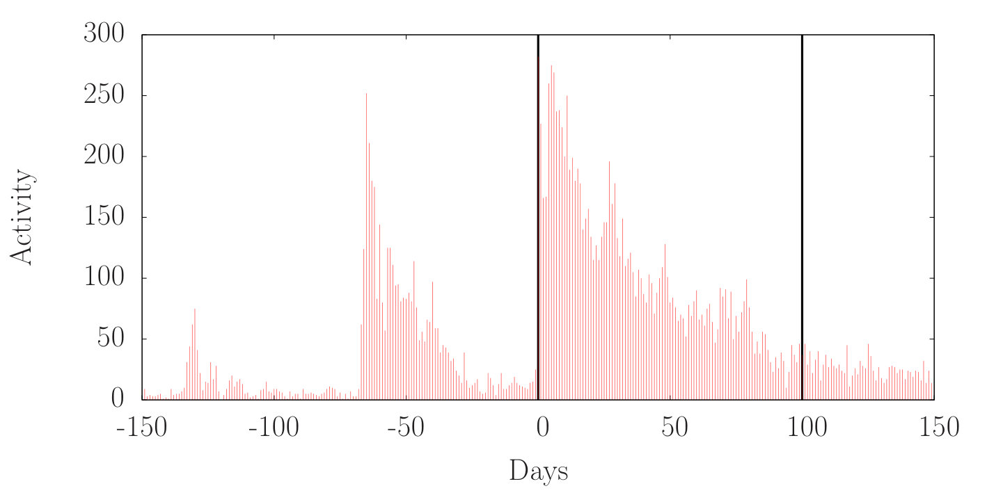 Figure 1
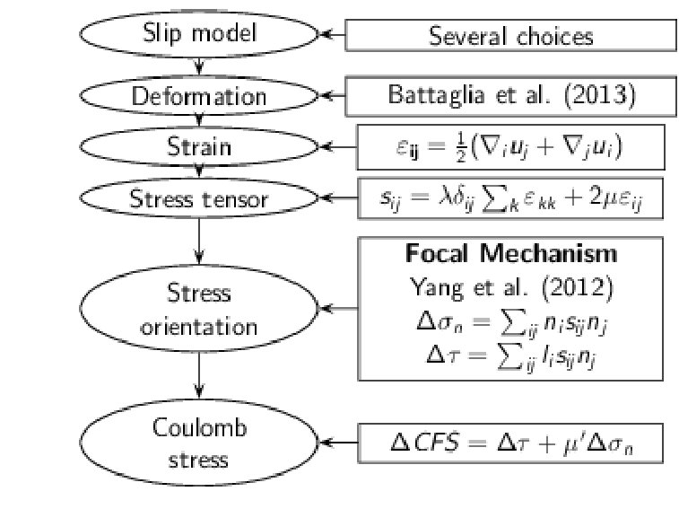 Figure 2
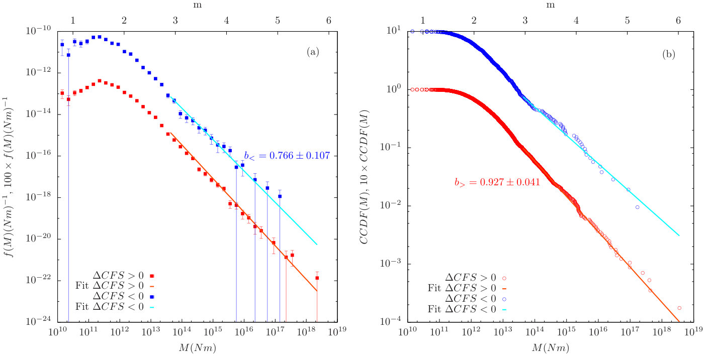 Figure 3
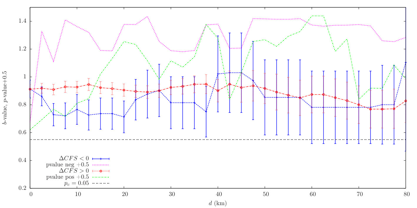 Figure 4
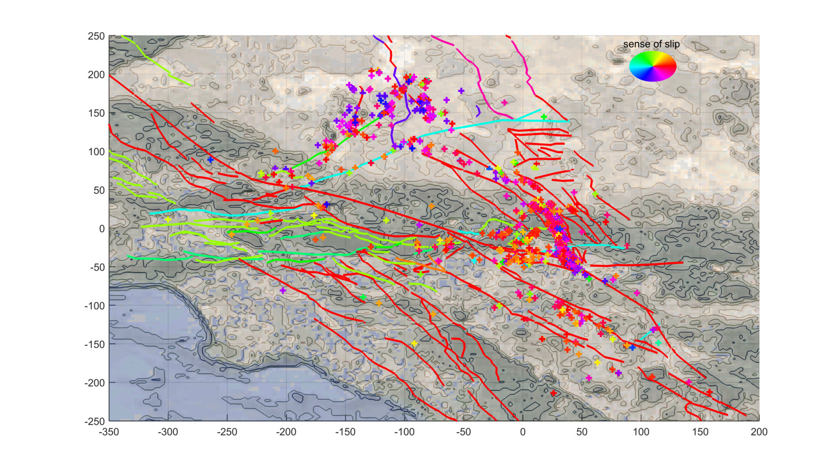 Figure 5
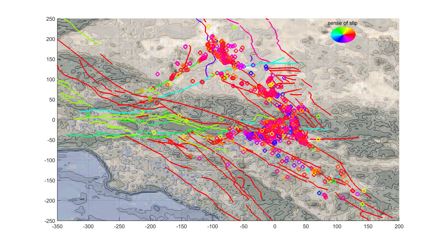 Figure 6
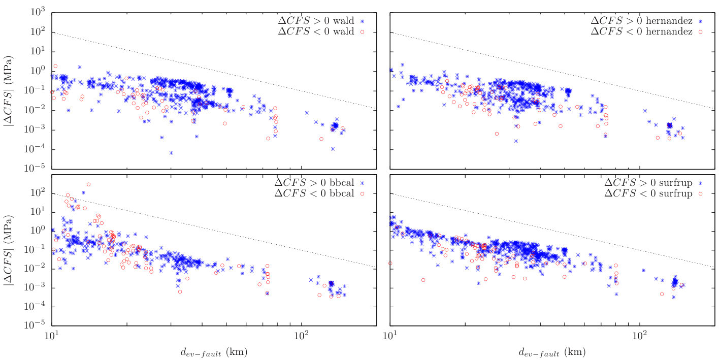 Figure 7
| Slip Model | value | |||||
|---|---|---|---|---|---|---|
| wald | 5213 | 509 | 0.041 | |||
| 814 | 51 | 0.107 | ||||
| All | 6027 | 560 | 0.038 | |||
| hernandez | 5027 | 465 | 0.043 | |||
| 765 | 62 | 0.110 | ||||
| All | 5792 | 527 | 0.040 | |||
| bbcal | 3641 | 309 | 0.056 | |||
| 1191 | 82 | 0.105 | ||||
| All | 4832 | 391 | 0.049 | |||
| surfrup | 5534 | 548 | 0.038 | |||
| 774 | 68 | 0.108 | ||||
| All | 6308 | 616 | 0.036 |
| Slip Model | ||||||
|---|---|---|---|---|---|---|
| wald | 1.396 | 0.163 | 0.139 | 0.311 | 0.234 | |
| hernandez | 0.511 | 0.609 | 0.095 | 0.690 | 1.748 | |
| bbcal | 0.254 | 0.800 | 0.063 | 0.952 | 1.936 | |
| surfrup | -0.010 | 0.992 | 0.094 | 0.643 | 1.999 |
| fm | ||||||||
| wald | ||||||||
| No: | 39 | 5 | 1.047 | - | ||||
| Th: | 9 | 8 | - | - | ||||
| SS: the rest | 461 | 38 | 0.914 | 0.726 | ||||
| hernandez | ||||||||
| No: | 38 | 3 | 0.995 | - | ||||
| Th: | 7 | 10 | - | - | ||||
| SS: the rest | 420 | 49 | 0.920 | 0.840 | ||||
| bbcal | ||||||||
| No: | 22 | 4 | 1.128 | - | ||||
| Th: | 7 | 5 | - | - | ||||
| SS: the rest | 280 | 73 | 0.970 | 0.886 | ||||
| surfrup | ||||||||
| No: | 46 | 5 | 0.939 | - | ||||
| Th: | 9 | 11 | - | 1.010 | ||||
| SS: the rest | 493 | 52 | 0.888 | 0.844 |
| value | |||||
|---|---|---|---|---|---|
| Overall | 6730 | 662 | 0.034 | ||
| , | 5554 | 564 | 0.038 | ||
| , | 1176 | 98 | 0.077 | ||
| , | 5632 | 573 | 0.038 | ||
| , | 1098 | 89 | 0.078 | ||
| , | 5678 | 580 | 0.038 | ||
| , | 1052 | 82 | 0.081 | ||
| , | 5670 | 582 | 0.038 | ||
| , | 1060 | 80 | 0.082 | ||
| , | 5603 | 583 | 0.038 | ||
| , | 1127 | 79 | 0.083 |
Peer Reviews
No public reviews on file for this paper yet. If you reviewed it on a platform where reviews are public (OpenReview, ICLR, NeurIPS, ICML), you can paste yours below so the community can read it here.
Videos
No videos yet. Explain this paper in a talk, walkthrough, or lecture? Add one.
.
No Significant Effect of Coulomb Stress on the Gutenberg-Richter Law after
the Landers Earthquake
Víctor Navas-Portella
Centre de Recerca Matemàtica, Edifici C, Campus Bellaterra, E-08193 Barcelona, Spain
Barcelona Graduate School of Mathematics, Edifici C, Campus Bellaterra, E-08193 Barcelona, Spain
Facultat de Matemàtiques i Informàtica, Universitat de Barcelona, Barcelona, Spain
Abigail Jiménez
Departamento de Computación e Inteligencia Artificial. Universidad de Granada. Campus Ceuta C/. Cortadura del Valle s.n., 51001 Ceuta, Spain
Álvaro Corral
Centre de Recerca Matemàtica, Edifici C, Campus Bellaterra, E-08193 Barcelona, Spain
Barcelona Graduate School of Mathematics, Edifici C, Campus Bellaterra, E-08193 Barcelona, Spain
Departament de Matemàtiques, Universitat Autònoma de Barcelona, E-08193 Barcelona, Spain
Complexity Science Hub Vienna, Josefstädter Strae 39, 1080 Vienna, Austria
Abstract
Coulomb-stress theory has been used for years in seismology to understand how earthquakes trigger each other. Whenever an earthquake occurs, the stress field changes, and places with positive increases are brought closer to failure. Earthquake models that relate earthquake rates and Coulomb stress after a main event, such as the rate-and-state model, assume that the magnitude distribution of earthquakes is not affected by the change in the Coulomb stress. By using different slip models, we calculate the change in Coulomb stress in the fault plane for every aftershock after the Landers event (California, USA, 1992, moment magnitude 7.3). Applying several statistical analyses to test whether the distribution of magnitudes is sensitive to the sign of the Coulomb-stress increase we conclude that no significant effect is observable. Further, whereas the events with a positive increase of the stress are characterized by a much larger proportion of strike-slip events in comparison with the seismicity previous to the mainshock, the events happening despite a decrease in Coulomb stress show no relevant differences in focal-mechanism distribution with respect to previous seismicity.
Introduction
Since the L’Aquila event in 2009 seismologists have advocated the modeling and testing of earthquakes within a rigorous statistical framework Jor11 , following on the CSEP (Collaboratory for the Study of Earthquake Predictability) previous works. A recent pseudo-prospective forecast was conducted on the 2010-2012 Canterbury, New Zealand, series, in order to test a total of fourteen earthquake models Werner2015 ; MW18 . Its results offer some encouragement for a physical basis in earthquake forecasting and suggest that some of the recent physics-based and hybrid model development have added informative components Cattania2018 .
Our basic understanding of earthquake physics is that stress is being accumulated on certain regions due to different mechanisms, and that those regions rupture whenever that stress surpasses the strength of the material. That rupture is the earthquake. The mechanisms by which stresses change are diverse: in addition to tectonic driving, they can be induced by precedent earthquakes Stein1992 ; King1994 ; Steacy2005 ; Nandan2016 ; Ishibe2015 , by volcanic activity JGRB:JGRB50413 , or even by artificial means, such as injection of fluids GonzalezCastor2014 or aquifer withdrawal Shirzaei1416 . Coulomb-stress theory has been used to forecast spatial patterns of aftershock rates, as well as assessing the likelihood of earthquake rupture sequences Quigley2019 ; Par00 . Although there exist instances where its predictive skills are arguable Hardebeck_jgr ; Marsan2003 ; doi:10.1029/2005JB004076 ; doi:10.1029/2004JB003277 , the monitoring of the changes in the stress field represents a valuable information for seismic and volcanic hazard forecasting and to proposing the adequate mitigation measures.
A hallmark of statistical seismology and of earthquake hazard assessment is the well-known Gutenberg-Richter relation, or Gutenberg-Richter law GR44 ; Utsu_GR ; Kagan_book . This law states that earthquake magnitudes must be described in terms of a probability distribution and that, above a lower cut-off value, this distribution is exponential. In terms of the probability density one has
[TABLE]
defined for (values below are disregarded), with the magnitude, the lower cut-off in magnitude, the so called value (directly related to the exponent of the power-law cumulative distribution of seismic moment, ), and the symbol denoting proportionality. (This relation is usually called magnitude-frequency distribution in seismology). A straightforward property of the exponential distribution leads to the fact that the rate (the number per unit time of earthquakes above a certain magnitude ) is also a decreasing exponential function of the magnitude, with the same value.
Earthquake hazard forecasts usually comprise two stages: in the first one, the rate of events is forecasted, while in the second one, the Gutenberg-Richter law is applied to those rates in order to obtain the probabilities of occurrence for each magnitude threshold. In the case of physics-based models, the forecasted rates of events depend on the Coulomb stresses calculated in the region of interest. These models are variants of the rate-and-state model by Dieterich JGRB:JGRB9328 ,
[TABLE]
where is the rate of events (i.e., aftershocks) at any given time after a mainshock, is the rate of background seismicity, is the increase in Coulomb stress induced by the mainshock, is a constant, for our purposes, and is the characteristic relaxation time JGRB:JGRB9328 .
Note that in the application of the Gutenberg-Richter law to the forecasted rate given by the previous expression it is implicit that the Coulomb-stress change caused by a mainshock does not alter the fufillment of the Gutenberg-Richter law for the aftershocks, in particular, this law remains the same no matter whether is positive or negative. In some sense, inherites the dependence of the background rate with the magnitude. Therefore, the rate-and-state formulation JGRB:JGRB9328 ; Par00 ; Tod05 ; Cha12 ; Cat14 ; Cat15 assumes the fulfillment of the Gutenberg-Richter law for the incoming events (aftershocks), with no change in the value. This assumption is made when inverting earthquake rates to obtain stress changes SA00 ; DCO00 ; JGRB:JGRB50413 . Physics-based models also assume the magnitude distribution does not depend on the stress values, so that forecasted rates can be translated into probabilities of occurrence for different magnitudes.
In fact, it has been long debated Kamer whether the value of in the Gutenberg-Richter law is essentially universal Kagan_book or whether, on the contrary, it is affected by different geophysical conditions. Some studies Sch05 ; Nar09 have correlated the value (and also the parameters of the Omori law Omo94 ; Uts61 ; Utsu_omori ) with the style of faulting Wyss1334 . These studies indicate that (at least for California, for a long time period) for normal events, for strike-slip events, and for thrust events Sch05 . As the value is directly related to the log-ratio between the number of small and large earthquakes, variations in can be associated with the ability of an earthquake rupture to propagate (more large events, low ) or not (less large events, high ).
According to Mohr-Coulomb theory Nar09 ; KB04 , thrust faults rupture at much higher stress than normal faults (with strike-slip faults in between, assuming the same value for the coefficient of static friction). When the stress required to initiate a rupture is higher, stress interactions are enhanced and cracks can propagate faster in many different directions, yielding larger earthquakes Nar09 , consistent with the empirically observed values for thrust faulting Sch05 . Conversely, for lower rupture thresholds, one should find indeed the large values characterizing normal faulting. Although the threshold for triggering might be different for the different styles of faulting, the rupture or not of a fault also depends on its previous state.
Here we investigate, with rigorous statistical tools, if the Gutenberg-Richter law is affected by the binary choice between positive and negative increases of the Coulomb stress, using the sequence of events after the 1992 Landers earthquake. The next section explains the seismic catalog and the spatio-temporal window used to define this sequence. Section 3 develops the procedure to calculate the increase in the Coulomb stress that the Landers earthquake provokes in the fault plane of each event in the sequence. The statistical analysis is also exposed in this section. Section 4 presents the results and Sec. 5 summarizes the conclusions.
Data
The June 28, 1992, Landers earthquake, with a moment magnitude and a rake angle , corresponding to strike-slip focal mechanism, has been the strongest one in Southern California at least since 1952. The earthquake and its subsequent aftershock sequence have been extensively studied Hill1617 ; JGRB:JGRB9241 ; Gombberg2001 , with a number of slip distributions that describe its rupture Wald01061994 ; bruno1999 ; Steacy2004 ; Spotila1995 . In this work we use four slip models to calculate the strain; these models are: Wald and Heaton (referred here to as wald)Wald01061994 , Hernandez et al. (hernandez) bruno1999 , Landers Big-Bear California (lbbcal) Steacy2004 and Landers Surface Rupture (lsurfrup) Spotila1995 . The terminology is the same as the one used in Ref. Steacy2004 .
High quality catalogs for Southern California are nowadays available 2012BuSSA.102.2239H ; PhysRevE.92.022808 ; in particular in this paper we will select the Landers’ aftershocks from the Yang-Hauksson-Shearer (YHS) catalog 2012BuSSA.102.1179Y , which incorporates focal-mechanism solutions. Given the distribution of acceptable mechanisms, the preferred solution is the most probable one Hardebeck2002 . The ambiguity of the actual fault plane is solved by considering that the preferred nodal planes are those associated with the preferred solution listed in the catalog 2012BuSSA.102.1179Y . The focal mechanism, in concrete, the rake angle, together with Landers stress field derived from the slip model, allows us to calculate Coulomb-stress increases (positive or negative) induced by the mainshock on the actual orientations of the aftershock ruptures. Note that the YHS catalog does not report the moment magnitude necessarily but a preferred magnitude.
In order to better detect the influence of the Landers stress change we take a time window of 100 days after the mainshock and a spatial window going from 10 to 150 km from the Landers rupture. Landers earthquake is taken as the mainshock for all the slip models except for the lbbcal whose mainshock is the Big-Bear earthquake (which occurred approximately three hours after Landers earthquake with a moment magnitude and rake angle Steacy2004 ). We tried other choices for the limits of the window finding similar results as reported in the Supplementary Material. This spatio-temporal window defines Landers aftershocks for our purposes. Distances to the fault are computed as the minimum Euclidean distance from the aftershock hypocenter to the center of each fault patch as given by the slip model. The reason to exclude events closer than 10 km is the uncertainty of the deformation field near the edges of the subfaults Okada92 , as the finite-fault approximation provides spurious values near the fault zone because of boundary effects.
Procedure
The dMODELS software in Ref. Battaglia20131 calculates the deformation field (or displacement) caused by different models corresponding to different physical processes. Although there exist many programs that calculate deformation caused by earthquakes, this package has been thoroughly tested, and can introduce many different sources of deformation, which can be translated into stress changes in a straightforward way. The dMODELS software will be the one used here to obtain deformation field from the different slip models of Landers.
The local coordinate system for dMODELS is east-north-up, ENU. After introducing the corresponding slip model (also called source model) for the mainshock of interest (Landers in our case Steacy2004 ) into the dMODELS program we obtain the projections in the ENU axes of the deformation field caused by the mainshock at the position of each aftershock (and also at its neighborhood, in order to take spatial derivatives). We then obtain the strain tensor associated to by calculating the (symmetrized) gradient of the deformation Lautrup , whose components are (with a spatial step equal to km).
Afterwards, we assume an isotropic and elastic material for calculating the stress tensor Lautrup , or, more precisely, the contribution of the mainshock to the stress tensor, , with the components of the identity matrix and with the Lamé elastic moduli given by MPa KB04 (Poisson ratio ). Moreover, when calculating the stress induced by previous events (mainshocks) on new events (aftershocks) it is necessary to orientate it onto the fault GRL:GRL16929 ; TOTS17 , so that one can actually evaluate if the new events could have been triggered by the induced stress or not. Given the fault plane and slip vector of an aftershock, we calculate the change in the normal and shear (or tangential) stresses in that orientation and position, as
[TABLE]
with and the components of the normal and slip vectors, respectively. The formulas to obtain the ENU components of these vectors from the information recorded in the YHS catalog (strike, dip and rake angles akirichards ) are given in the Methods section. Note that in order to be realistic, the Coulomb-stress changes have to be calculated onto the planes of the actual faults GRL:GRL16929 . This contrasts with an approach in which Coulomb stresses are calculated onto the so-called optimally oriented planes King1994 , when the only information available is the regional stress. However, optimally oriented planes are imaginary planes that might not correspond to the actual geology.
The Mohr-Coulomb failure criterion vavryvcuk2015earthquake states that the shear stress on a fault that ruptures must surpass the critical value , which is a linear function of the normal stress,
[TABLE]
with the cohesion and the effective fault friction coefficient (including the contribution of the pore pressure JGRB:JGRB12887 ; King1994 ). Care must be taken with the convention of signs in the normal stress, which is not the same in geophysics than in solid mechanics (our convection takes the negative sign for compression, this is the reason for the negative sign before ). From this failure criterion it is natural to define the Coulomb stress as which signals failure by . In fact, for pre-existing faults one can consider that the cohesion is nearly zero. The change in Coulomb stress at the aftershock fault plane due to the mainshock will be
[TABLE]
with and coming from Eq. (2). Thus, positive increases of the Coulomb stress bring the fault closer to failure, whereas negative increases distance it away from failure.
As the real value of the effective friction coefficient is uncertain KB04 , we will check different values of it as in Ref. Hardebeck_jgr . In Fig.1 we present a scatter plot that illustrates the dependence of the absolute value of the increase of Coulomb stress as a function of the distance to the fault for the four slip models. As it is implicit by the Coulomb theory, the value of the increase of Coulomb stress decays as the cube of the distance to the fault. In Fig.2 we show aftershocks with positive and negative increase of Coulomb stress placed in the window we study for the wald slip model and .
Once we know the Coulomb-stress change in the fault plane of each aftershock we can separate these into two subsets attending to the value of the change, with the most natural separation being between positive and negative increases (denoted by sub-indexes and , respectively). Naturally, we expect to obtain many more aftershocks in positive lobes than in negative ones Stein_nature . It is for each of these subsets that we will study the fulfilment of the Gutenberg-Richter law. For any set or subset (or sub-catalog) of earthquakes, the value of in the Gutenberg-Richter law can be automatically obtained by maximum-likelihood estimation, asAki_mle ; Marzocchi_bvalue :
[TABLE]
with the mean magnitude of the events considered (i.e., those above ). Let us stress that is not the minimum magnitude recorded in the catalog but the value from which we fit the Gutenberg-Richter law to the data. As the resolution of the magnitude is small () it is not necessary to perform the discreteness correction Bender1983 .
In principle, results should not significantly depend on the value of , but the larger its value the less data to calculate the value and the larger the uncertainty, whereas for a too small the Gutenberg-Richter law would not be fulfilled due to the incompleteness of the catalog and the resulting value would be artefactual. In this paper we have taken , which ensures the fulfilment of the Gutenberg-Richter law for all data sets analysed, as we have verified by means of the Kolmogorov-Smirnov goodness-of-fit test Press , where the distribution of the test statistic and, from it, the value of the fit, , is calculated using Monte Carlo simulations Clauset ; Corral_Deluca . Although some fitting procedures look for the value of that optimizes the fit for a given data set Clauset ; Corral_Deluca ; CorralGonzalez2019 , we have opted for a fixed in order to compare the different subsets on the same footing. So, in all cases the exponential fit for cannot be rejected (value of the test larger than 0.05). Note that defined in this way can be considered a magnitude of completeness, and thus, our value of turns out to be rather conservative or strict, in the sense that it is larger (and therefore safer) than in other works Woessner2005 .
The maximum-likelihood estimation of the value has an associated uncertainty given by its standard deviation
[TABLE]
where is the number of earthquakes with in the subset, out of a total number (of any magnitude)ShiBolt1982 . Note that this uncertainty only depends on the number of data, and has nothing to do with the goodness of the fit. This result, as well as the formula for the maximum-likelihood estimation of , Eq. (5), can also be obtained from Ref. Corral_Deluca just taking into account the relation between moment magnitude and seismic moment. This standard deviation, , is what represents the uncertainty when we report our resulting -values.
The comparison between the values of the subsets with different values of is done by means of the following statistic
[TABLE]
where the sub-indexes and refer to positive and negative increases of the Coulomb stress. This statistics is rooted on the null hypothesis that both subsets of data (positive and negative) belong to the same underlying population of earthquake magnitudes and then, both estimators of the value ( and ) have a common mean value, which is that of the whole population. Therefore, under the null hypothesis, has zero mean and standard deviation (approximating the population variance from the sample values of and and assuming zero covariance between and ) and then has zero mean too and unit standard deviation. An additional assumption is that is normally distributed, which is supported by theory in the asymptotic limit ( and going to infinity pawitan2001 ). Assuming normality we will test the null hypothesis just comparing the value of with the standard normal distribution and the hypothesis will be rejected if the value of is too extreme for a given significance level; in quantitative terms this will be given by a value, called , smaller than the significance level (0.05, let us say; corresponding to 0.95 confidence).
If we do not want to believe that the asymptotic regime has been reached the best option is to use a permutation test Good_resampling . Under the null hypothesis (all values of magnitude belong to the same population) one is allowed to aggregate both subsets (positive and negative) and take, without repetition, two sub-samples of size and ; note that this is equivalent to take a permutation of the aggregated sample and separate it into two parts ( and ). One proceeds in the same way as in the original data, calculating (by maximum likelihood) , , and from here , , and , where the asterisk marks that we are dealing with a permutation of the original data. Repeating the permutation procedure many times we find the distribution of , which can be compared with the original value . The value of the permutation test, , will be given by the fraction of permutations for which is larger than (the empirical value). In our case we take permutations.
As a complement, instead of the fitted values we may directly compare the distributions; this can be done with the two-sample Kolmogorov-Smirnov test, whose null hypothesis is that both data sets come from the same population, so, the two empirical distributions ( and ) are two realizations of a unique theoretical distribution (which remains unveiled) Press . This test leads to a -value that we call . A final comparison comes from the application of the Akaike information criterion () AICBOOK . We consider that we aggregate both subsets (positive and negative ) but keeping the distinction in the sign of . Then, we contemplate two options. Model 1, simple: we fit the aggregated data set with one single Gutenberg-Richter exponential leading to the value . Model 2, “complex”: we fit each data set with its own exponential function (values and in the same table). In each case, , where is the number of parameters of each model and is the log-likelihood of the model at maximum. The likelihood in model 2 is the sum of likelihoods for each subcatalog pawitan2001 . The model yielding the smallest should be prefered. Defining leads to the rejection of the simple model when is significantly below zero (see next section).
Results
Table 1 shows the values of obtained from the application of the maximum likelihood estimation and goodness-of-fit test explained above to the different subcatalogs obtained from the Landers sequence. We can see how, in the overall case (when events are not separated in terms of Coulomb-stress change), the Gutenberg-Richter law is fulfilled with an average value . Each slip model leads to a different value of because the fault geometry is different, and events too close to the fault are discarded. This value for the Landers aftershocks is found, not surprisingly, to be close to the average for aftershocks in California, Reasenberg_Jones89 ; Jones1994 , and somewhat below the long-term value of Southern California (all events), Hutton_Woessner (although other works report for Landers aftershocks, probably due to the consideration there of a much smaller magnitude of completeness Shcherbakov2005 ).
After separating by the sign of the Coulomb-stress change, the first result that becomes apparent from the table is that the number of aftershocks with positive increases is much larger than the number for the negative case King1994 ; Steacy2005 , no matter neither the slip model (nor the value of ) used to calculate . Regarding the values, although they depend on the slip model, we can summarize them by taking the mean of the four models and taking as and with individual uncertainties around and respectively. Note that the magnitude distribution for the overall case is a mixture of the distributions corresponding to and , and therefore, the value of in the overall case turns out to be the harmonic mean of and , i.e.,
[TABLE]
see Refs. hernandez2014; Navas_pre2 . Despite the fact the values of and do not look much different between them, statistical testing becomes necessary in order to establish significance Corral_Boleda .
Table 2 compares and for the different slip models taking , and shows that the difference in the values can not be considered significantly different from zero with a confidence larger than so, the null hypothesis can not be rejected. This result is true for all the statistical tests as all the -values are greater than . Table 2 also shows the results of the two-sample Kolmogorov-Smirnov test and the calculation of leading in both cases to the result that no change in the distributions as a function of positive and negative can be established. In concrete, is always greater than the critical value AICBOOK ; Murtaugh2014 at significance level of . The wald slip model is the one for which both distributions (positive and negative) appear as more different; however, the difference is not significant. Figure 3 shows the probability density functions as well as the complementary cumulative probability functions in this case.
As mentioned in the introduction, some authors have unveiled a direct dependence of the value on the focal mechanism of the events, which implies a dependence of on the total stress (not the stress increase) Sch05 . The rake angle is associated to the focal mechanism in the following way: values of the rake around correspond to normal events (labelled as ), values around or to strike-slip events (), and values around to thrust events (). We do not find any significant effect of the rake on the value (See Table 3), due to the low number of events in the normal and thrust regimes (which increases the uncertainty). But despite the large uncertainty, the values of and are roughly in agreement with the results of Ref. Sch05 ; however, our value of turns out to be rather large in comparison (but compatible, within the error bars). We further observe that ratios and are higher than ; i.e., in strike-slip and normal events the contribution from is higher than in thrust events, as can be verified looking at Table 3. Comparing with the number of earthquakes with each focal mechanism for the 5 years previous to Landers we conclude that it is indeed the low number of thrust aftershocks with positive which is anomalous (and not the relatively high number of them for negative ), due to an increase in the number of normal events and an even higher increase in strike-slip events triggered () by the Landers mainshock. This difference in numbers becomes visually apparent in Fig. 2.
Discussion
We have seen how the positive Coulomb-stress increase associated to the Landers mainshock triggered a very large number of strike-slip events and also a large number of normal events, but much less thrust events. Although this result seems easy to establish, as it can be obtained without the calculation of (due to the fact that most of the events have and thus, this subset dominates the overall statistics), we have unambiguosly associated these events to the positive . On the other side, the events in the opposite regime (with ) keep a proportion between normal, strike-slip, and thrust events rather different to the case, and close to that of the immediately previous record (1987-1992, up to Landers). These results are largely independent on the slip model used to calculate the change in Coulomb stress. We have also found that the -values of the Gutenberg-Richter law for events with positive (for which ) are in general larger than the values for the events with negative (); nevertheless, this difference is not statistically significant for any of the slip models used to compute the change in the Coulomb stress.
A number of extensions and improvements could be incorporated to our approach in future research. Moreover, we need to take into account the relation between -values and differential stress amitrano2003 . We make use of slip models with relatively low resolution in space; so, it would be interesting to know if higher resolution slip models Olsen1997 ; Peyrat2001 lead to somewhat different values of the strain and the stress, in particular close to the fault. Also, some authors have argued that real faults should have rather low values of the coefficient Mulargia2016 . We provide some check of this in the supplementary material, which leads to the conclusion that has little influence on the values. Further, in our temporal window of 100 days, the effect of viscoelastic relaxation Sabadini2016 should be important; so, this would need to be incorporated into the calculation of the stress. Finally, in a preliminary analysis we have seen that there is no substantial difference in the fulfilling of the Omori law Omo94 ; Uts61 ; Utsu_omori in the two populations of events ( and ). Indeed, if we compare this for the two subsets we find the “characteristic” power-law Omori decay of the rate with very similar values of the Omori exponent. Note that this is in disagreement with the rate-and-state formulation JGRB:JGRB9328 , which does not predict Omori behavior in the case of negative . Certainly, more research using other mainshocks (for which detailed slip models were available) is necesary, in order to reduce the statistical uncertainty by means of aggregated distributions, which could lead to the detection of small significant differences in both populations of events.
Methods
The YHS catalog characterizes fault planes and slip vectors by means of three angles: strike , dip , and rake . In term of these, the normal vector of the fault is given by
[TABLE]
in the ENU coordinate system Smith2006 . In the same way, the slip vector is obtained as
[TABLE]
Note that and are unit vectors.
Supplementary Material
Acknowledgements
We are grateful to Álvaro González for some comments on the manuscript, to Paolo Gasperini, Francesco Mulargia, Fabio Romanelli and Roberto Sabadini for the feedback provided during the International Workshop on Seismic Source Physics, Sardinia, and to two anonymous referees who detected some problems in a previous version of the manuscript. The research leading to these results has received founding from “La Caixa” Foundation. V. N. acknowledges financial support from the Spanish Ministry of Economy and Competitiveness (MINECO, Spain), through the “María de Maeztu” Programme for Units of Excellence in R & D (Grant No. MDM-2014-0445). We also acknowledge financial support from MINECO and MICIU under Grants No. FIS2015-71851-P, FIS-PGC2018-099629-B-I00, and “Proyecto Redes de Excelencia” Grant No. MAT2015-69777-REDT. A. J. appreciates the hospitality of the Centre de Recerca Matemàtica.
Author contributions statement
V. N.-P. and A. J. performed the computations, A. J and A. C. wrote the manuscript. All authors discussed the results and reviewed the manuscript.
Competing interests
The authors declare no competing financial and non-financial interests.
The reference list from the paper itself. Each links out to its DOI / PubMed record.
- 1(1) T. H. Jordan, Y. T. Chen, P. Gasparini, R. Madariaga, I. Main, W. Marzocchi, G. Papadopoulos, G. Sobolev, K. Yamaoka, and J. Zschau. Operational Earthquake Forecasting. State of knowledge and guidelines for utilization. Annals of Geophysics , 54, 2011.
- 2(2) M. Werner, M. Gerstenberger, M. Liukis, W. Marzocchi, D. Rhoades, M. Taroni, J. Zechar, C. Cattania, A. Christophersen, S. Hainzl, A. Helmstetter, A. Jiménez, S. Steacy, and T. Jordan. Retrospective evaluation of time-dependent earthquake forecast models during the 2010-12 Canterbury, New Zealand, earthquake sequence. In Proceedings of the SSA Annual Meeting, Pasadena (USA) , 2015.
- 3(3) A. J. Michael and M. J. Werner. Preface to the focus section on the Collaboratory for the Study of Earthquake Predictability (CSEP): New results and future directions. Seism. Res. Lett. , 89(4):1226, 2018.
- 4(4) C. Cattania, M. J. Werner, W. Marzocchi, S. Hainzl, D. Rhoades, M. Gerstenberger, M. Liukis, W. Savran, A. Christophersen, A. Helmstetter, A. Jiménez, S. Steacy, and T. H. Jordan. The forecasting skill of physics-based seismicity models during the 2010-2012 Canterbury, New Zealand, earthquake sequence. Seism. Res. Lett. , 89(4):1238, 2018.
- 5(5) R.S. Stein, G.C.P. King, and J. Lin. Change in failure stress on the southern San Andreas fault system caused by the 1992 magnitude=7.4 Landers earthquake. Science , 258:1328–1332, 1992.
- 6(6) G. King, R. S. Stein, and J. Lin. Static stress changes and the triggering of earthquakes. Bull. Seismol. Soc. Am. , 84:935–953, 1994.
- 7(7) S. Steacy, J. Gomberg, and M. Cocco. Introduction to special section: stress transfer, earthquake triggering, and time-dependent seismic hazard. J. Geophys. Res. , 110:B 05S 01, 2005.
- 8(8) S. Nandan, G. Ouillon, J. Woessner, D. Sornette, and S. Wiemer. Systematic assessment of the static stress triggering hypothesis using interearthquake time statistics. J. Geophys. Res.: Solid Earth , 121:1890–1909, 2016.