Haj\'os-Type Constructions and Neighborhood Complexes
Benjamin Braun, Julianne Vega

TL;DR
This paper explores Hajós-type graph constructions and their impact on neighborhood complexes, revealing restrictions for highly-connected complexes and introducing algorithms with computational experiments.
Contribution
It demonstrates the frequent emergence of $S^1$-wedge summands in neighborhood complexes during Hajós-type constructions and introduces new algorithms for graph construction.
Findings
Presence of $S^1$-wedge summands in neighborhood complexes
Restrictions on construction sequences for highly-connected complexes
Development and testing of new graph construction algorithms
Abstract
Any graph with chromatic number can be constructed by iteratively performing certain graph operations on a sequence of graphs starting with , resulting in a variety of Haj\'os-type constructions for . Finding such constructions for a given graph or family of graphs is a challenging task. We show that the basic steps in these Haj\'os-type constructions frequently result in the presence of an -wedge summand in the neighborhood complex of the resulting graph. Our results imply that for a graph with a highly-connected neighborhood complex, the end behavior of the construction sequence is quite restricted, and we investigate these restrictions in detail. We also introduce two graph construction algorithms based on different Haj\'os-type constructions and conduct computational experiments using these.
Click any figure to enlarge with its caption.
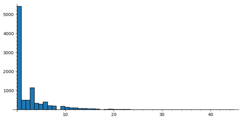 Figure 1
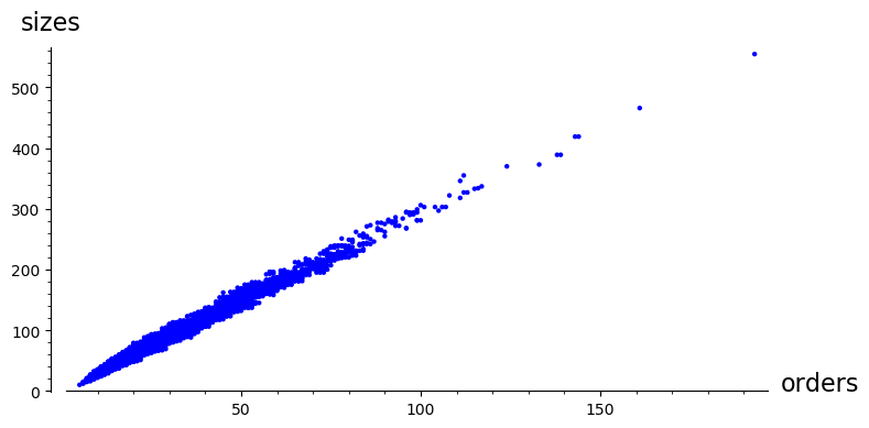 Figure 2
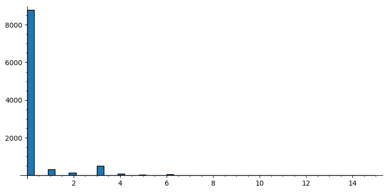 Figure 3
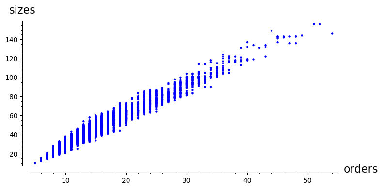 Figure 4
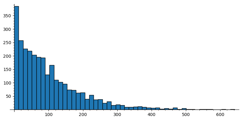 Figure 5
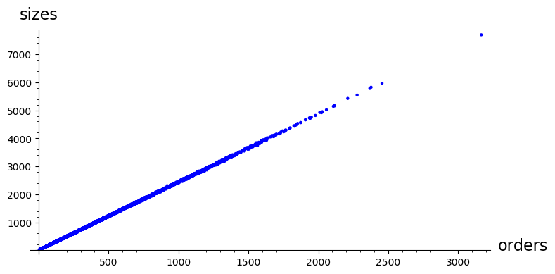 Figure 6
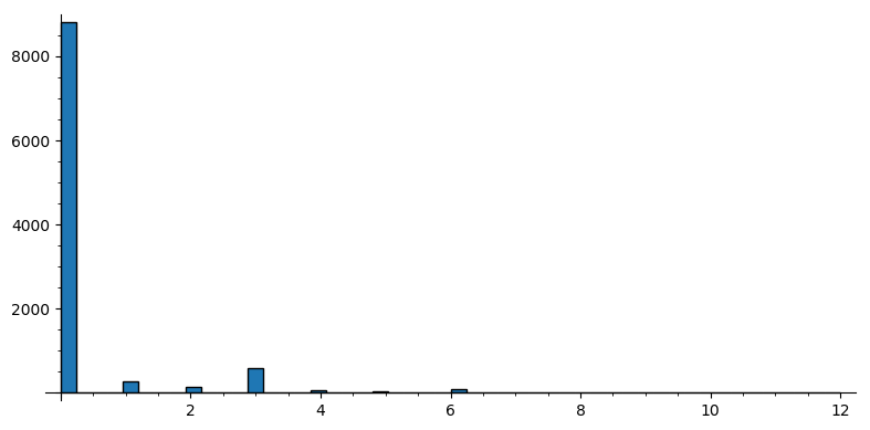 Figure 7
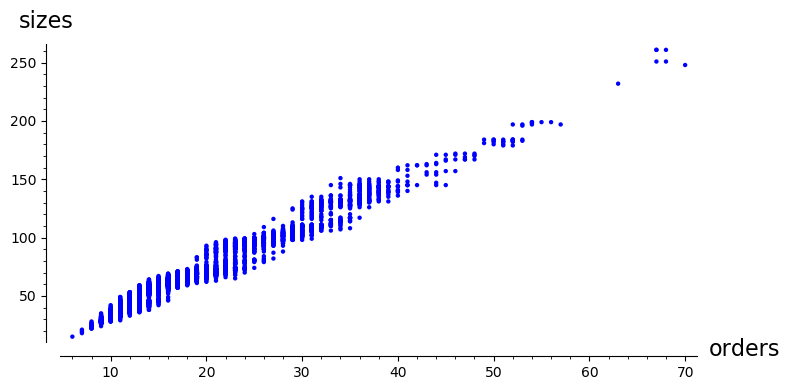 Figure 8
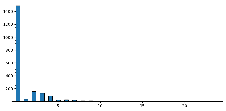 Figure 9
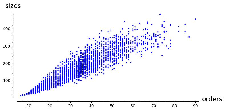 Figure 10
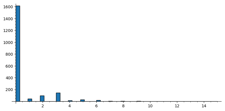 Figure 11
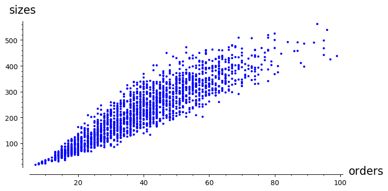 Figure 12
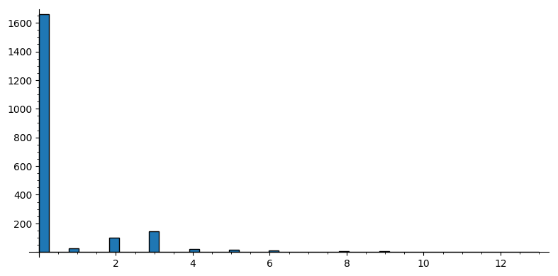 Figure 13
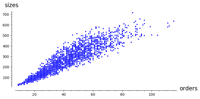 Figure 14
| # graphs generated | fraction of first Betti numbers equal to zero | ||
|---|---|---|---|
| 10,000 | 0.25 | ||
| 10,000 | 0.065 | ||
| 10,000 | 0.0018 | ||
| 10,000 | 0.61 | ||
| 10,000 | 0.32 | ||
| 10,000 | 0.01 | ||
| 10,000 | 0.88 | ||
| 10,000 | 0.54 | ||
| 2,939 | 0.03 | ||
| 10,000 | 0.88 | ||
| 10,000 | 0.44 | ||
| 2,894 | 0.08 |
| # graphs generated | fraction of first Betti numbers equal to zero | |
| 0.67 | ||
| 0.74 | ||
| 0.81 | ||
| 0.83 |
Peer Reviews
No public reviews on file for this paper yet. If you reviewed it on a platform where reviews are public (OpenReview, ICLR, NeurIPS, ICML), you can paste yours below so the community can read it here.
Videos
No videos yet. Explain this paper in a talk, walkthrough, or lecture? Add one.
Hajós-Type Constructions and Neighborhood Complexes
Benjamin Braun
Department of Mathematics
University of Kentucky
Lexington, KY 40506–0027
and
Julianne Vega
Department of Mathematics
University of Kentucky
Lexington, KY 40506–0027
(Date: 18 December 2018)
Abstract.
Any graph with chromatic number can be constructed by iteratively performing certain graph operations on a sequence of graphs starting with , resulting in a variety of Hajós-type constructions for . Finding such constructions for a given graph or family of graphs is a challenging task. We show that the basic steps in these Hajós-type constructions frequently result in the presence of an -wedge summand in the neighborhood complex of the resulting graph. Our results imply that for a graph with a highly-connected neighborhood complex, the end behavior of the construction sequence is quite restricted, and we investigate these restrictions in detail. We also introduce two graph construction algorithms based on different Hajós-type constructions and conduct computational experiments using these.
1. Introduction
1.1. Motivation
Proper graph colorings are of great interest in combinatorics and the study of chromatic numbers for graphs is a frequent focus. While coarse bounds on the chromatic number can be found easily, determining the chromatic number is NP-complete. In 1978, Lovász advanced the study of chromatic numbers through the construction of the neighborhood complex of a graph . Intuitively, is capturing the relations of the vertices with their neighbors and the topological connectivity of is measuring the complexity of continuous deformations of the neighborhoods in the graph. Lovász [13] proved that the topological connectivity of gives a general lower bound for the chromatic number of , and then showed that this provides a sharp lower bound for Kneser graphs. Since this original result, there has been steady development regarding our understanding of neighborhood complexes of graphs and various topological lower bounds for chromatic numbers [10].
Another area of interest related to graph colorings is the characterization of -chromatic graphs, i.e. graphs with chromatic number . In 1961, Hajós [2] characterized graphs with chromatic number at least through the concept of a -constructible subgraph, where constructibility is defined recursively using the operations of vertex identification and Hajós merging. Strengthening this result, Urquhart [19] showed that every -chromatic graph is -constructible for . In the proof, Urquhart describes a Hajós-type construction which involves an “Ore merge,” an operation that involves the Hajós merge followed by a restricted series of vertex identifications.
Jensen and Royle [5] considered Hajós’ result in terms of -critical graphs. They proved that there exists -critical graphs that are not Hajós constructible through a sequence of -critical graphs. The proof of this result involved exploring the operations necessary for the final steps of the Hajós construction sequence, showing that the key to constructing -critical graphs is to end in a vertex identification.
Building on these narratives, we are led to ask in this article how the connectivity of the neighborhood complex of a given graph is affected by the Hajós merge and vertex identification operations. In addition, we ask what end behavior of Hajós construction sequences is necessary to obtain graphs with highly (topologically) connected neighborhood complexes.
1.2.
Our Contributions
We explore the topological effects of Hajós-type constructions from both theoretical and experimental perspectives. In Section 2, we discuss background for Hajós-type constructions, neighborhood complexes of graphs, and discrete Morse theory. We explore the topological effects of Hajós merges and vertex identifications in Section 3, providing insight into restrictions on Hajós-type constructions for graphs with highly connected neighborhood complexes. Our main result is Corollary 3.7, which states that such constructions must end with an identification of vertices at distance four or less from each other in the graph. Motivated by this, in Section 4 we investigate the impact of “short-distance” identifications on the first Betti number of . In Section 5, we briefly investigate the topological effects of DHGO compositions, a generalization of Hajós merges. Finally, in Section 6, we introduce two graph construction algorithms based on different Hajós-type constructions, discuss the outcomes of computational experiments using these, and conclude with open problems.
2. Background
2.1. Hajós-type Constructions
In this section we review Hajós-type constructions. Recall that a graph is -chromatic if it has chromatic number .
Definition 2.1**.**
A graph is called Hajós -constructible if it is a complete graph or if it can be constructed from by successive applications of the following two operations:
- •
(Hajós Merge) If and are already-obtained disjoint graphs, then to the disjoint union remove an edge from and an edge from , identify with , and add the edge . We abuse notation and denote the resulting graph .
- •
(Vertex Identification) Identify two nonadjacent vertices in an already-obtained graph , where we ignore the presence of multiple edges. If is a list of pairs of nonadjacent vertices in , then is the graph obtained by identifying all those pairs of vertices.
Any construction of a graph using this process will be called a Hajós construction. An example of a Hajós merge is given in Figure 1. It is straightforward to show that , and that . Thus, if is Hajós -constructible, then . Hajós proved further that if , then contains a Hajós -constructible subgraph.
Theorem 2.2** (Hájos [2]).**
For every , every -chromatic graph contains a -constructible subgraph.
Urquhart later strengthened Hajós’ result.
Theorem 2.3** (Urquhart [19]).**
For every , every -chromatic graph is -constructible.
This theorem has been the subject of continued investigation in recent years [3, 4, 5, 6, 11, 12, 19]. Urquhart proved Theorem 2.3 using a variant of Hájos’ construction that was introduced by Ore [15] as follows.
Definition 2.4**.**
A graph is Ore -constructible if it is a complete graph or if it can be constructed from by successive applications of the following operation:
- •
(Ore Merge) Suppose and are already-obtained disjoint graphs with respective edges and . Let be a bijection from a subset of to so that and , and . Form the Hajós merge on and using the two edges, then identify the vertex pairs . We abuse notation and denote the resulting graph .
Any construction of a graph using this process will be called an Ore construction.
Note that an Ore merge arises from a single Hajós merge followed by a sequence of restricted vertex identifications. However, Urquhart [19] proved that the families of Hajós constructible and Ore constructible graphs are equivalent.
Theorem 2.5** (Urquhart [19]).**
For a graph and , the following conditions are equivalent:
- •
* is Hajós--constructible;*
- •
* is Ore--constructible.*
In the proof of Theorem 2.5, Urquhart proved that for every -chromatic graph can be obtained by the following process.
Definition 2.6**.**
Suppose that a graph is obtained by applying Ore merges to a sequence of graphs each containing . We will call a construction of using this approach an Urquhart construction, and denote (again abusing notation) .
A -chromatic graph is -critical if every proper subgraph is -chromatic for some . Theorem 2.2 implies that -critical graphs are -constructible. Jensen and Royle [5] proved the existence of -critical graphs that do not have a Hajós sequence consisting of exclusively -critical graphs.
Theorem 2.7**.**
For every there exists a -critical graph that allows no Hajós -construction where all intermediary graphs are -critical.
The proof involves finding graphs that satisfy the three specifications in the proposition below for .
Proposition 2.8**.**
If
- (1)
is -connected, 2. (2)
has chromatic number at least , and 3. (3)
for every and every pair there exists a -coloring of such that for all ,
then is a -critical graph such that the last step of any possible Hajós -construction of consists of a vertex identification on a graph that is not critical.
2.2. Neighborhood Complexes
Recall that a simplicial complex on vertices is a collection of subsets of that is closed under containment and contains all singletons. We call an element of a face of . We will make no distinction between an abstract simplicial complex and an arbitrary geometric realization of as a topological space. A topological space is called -connected if for every , every continuous map from the boundary of , the unit ball in -dimensional Euclidean space, into can be extended to a continuous map from all of to . Equivalently, the higher homotopy groups vanish for all dimensions .
For any graph , Lovász [13] defined the neighborhood complex of , denoted , to be the simplicial complex with vertex set and facets given by for all , where denotes the neighbors of in (not including ). Lovász introduced in order to provide a sharp lower bound for the chromatic number of the Kneser graphs, which he did using the following theorem.
Theorem 2.9** (Lovász [13]).**
If is -connected, then .
There are several famous families of graphs, e.g. Kneser and stable Kneser graphs, for which these topological lower bounds (or equivalent techniques) yield the only known proofs of their chromatic numbers. Note that is [math]-connected if and only if it is path-connected, and being [math]-connected implies having chromatic number greater than . For connected bipartite graphs, having a disconnected characterizes this family. The following proposition justifies our assumptions throughout this work that when is connected with , is path-connected.
Proposition 2.10**.**
The complex is path-connected if and only if is connected and not bipartite.
Proof.
If is not connected, then it is immediate that is not connected. Let be a connected bipartite graph with bipartition , where denotes disjoint union. For all and for all . Therefore, the neighborhood complex induced by is disjoint from the neighborhood complex induced by and , hence is not connected.
Suppose now that is connected and not bipartite, so there exists an odd cycle in . We prove that between any two vertices there is a walk of even length, from which it follows that and are connected by a path in . Since is connected, there exists a walk from to some , and a walk from to some . Since has odd length, there exists a walk in of odd length from to , and there also exists a walk in of even length from to . For any given even/odd parities of and , one can connect and by a path of even length that starts with , continues through either or , and concludes with . Thus, and are path-connected in . ∎
In general, it is possible for there to be arbitrarily large gaps between and where is -connected, for example Matoušek and Ziegler [Remark (H1) in [14]] make a remark that implies the following.
Proposition 2.11**.**
If does not contain a -cycle, then is at most [math]-connected.
Thus, for example, the neighborhood complex for graphs with girth greater than are not -connected.
2.3. Discrete Morse Theory
Discrete Morse theory was first developed by R. Forman in [1] and has since become a powerful tool for topological combinatorialists. The main idea of the theory is to pair faces within a simplicial complex in such a way that we obtain a sequence of collapses yielding a homotopy equivalent cell complex.
Definition 2.12**.**
A partial matching in a poset is a partial matching in the underlying graph of the Hasse diagram of , i.e., it is a subset such that
- •
implies i.e. and no satisifies .
- •
each belongs to at most one element in .
When , we write and .
A partial matching on is called acyclic if there does not exist a cycle
[TABLE]
with and all being distinct.
Given an acyclic partial matching on a poset , an element is critical if it is unmatched. If every element is matched by , is called perfect. We are now able to state the main theorem of discrete Morse theory as given in [10, Theorem 11.13]
Theorem 2.13**.**
Let be a polyhedral cell complex and let be an acyclic matching on the face poset of . Let denote the number of critical -dimensional cells of . The space is homotopy equivalent to a cell complex with cells of dimension for each , plus a single [math]-dimensional cell in the case where the emptyset is paired in the matching.
It is often useful to create acyclic partial matchings on different sections of the face poset of a simplicial complex and then combine them to form a larger acyclic partial matching on the entire poset. This process is detailed in the following theorem known as the Cluster Lemma in [7] and the Patchwork Theorem in [10].
Theorem 2.14**.**
Assume that is an order-preserving map. For any collection of acyclic matchings on the subposets for , the union of these matchings is itself an acyclic matching on .
3. Topological effects of Hajós-type operations
In this section, we investigate the effects of Hajós merges and vertex identifications on , with our main result being Corollary 3.7. We assume throughout this section that and are connected graphs with chromatic numbers at least . We begin by showing the neighborhood complex is typically not -connected. Recall that a bridge in a graph is an edge whose deletion increases the number of connected components of .
Lemma 3.1**.**
* has a bridge if at least one of the edges used in the Hajós merge is a bridge.*
Proof.
Suppose and are two connected graphs with edges and respectively. Suppose under the Hajós construction and get identified as , while and get deleted and is added to create . Let . Suppose that is a bridge in such that , then the Hajos merge produces a graph with a bridge between and . ∎
Lemma 3.2**.**
Let be a connected non-bipartite graph such that is connected bipartite. Then, , where and .
Proof.
Since the deletion of the edge results in a bipartite graph, must be part of all the odd cycles and no even cycles in . Hence, by the connectivity of , there must be an even path from to and no such odd path. Therefore, there is no even path from to any neighbor or from to any neighbor , which implies and are not in the same connected component. Similarly for and . In addition, notice that and cannot be in the same component because they would need to be connected by an even path in creating an odd cycle, a contradiction to being bipartite. Similarly for and . Since a connected bipartite graph gives rise to a neighborhood complex with two connected components, the result follows. ∎
Theorem 3.3**.**
For two connected graphs and with edges and respectively such that either
- (1)
* and neither nor is a bridge or* 2. (2)
, , and is not a bridge,
* is homotopy equivalent to a wedge of at least one copy of with another space.*
Proof.
Suppose under the Hajós construction and get identified as , while and get deleted and is added to create . Let .
First, consider the effect of identifying and . Since and are elements in separate connected components, merging the two vertices in the disjoint union is homotopy equivalent to attaching a -cell between and , as shown in Figure 2. In addition, merging and has the effect of joining the faces and in , which adds to . Since , this join connects a face of to a face of through a contractible join which is homotopy equivalent to attaching a -cell between the contractions of and , respectively.
Now, let’s consider the effect of adding edge . Notice and , so adding the edge has the effect of coning over . Since is contractible, this is homotopy equivalent to attaching a -cell between and the contraction of . The analysis is similar for and , as shown in Figure 2.
We turn our attention to the number of connected components for and . Suppose is 0-connected (i.e. ). To obtain a copy of , at least one of the connected components of must contain at least two elements from the set , which follows from Lemma 3.2 when . So it suffices to consider
Suppose both and have two connected components, respectively. Let and . From Lemma 3.2 we can assume and . It follows that, up to homotopy equivalence, the Hajós construction attaches 1 -simplices between and , and , and , and and .
Thus, we have found that is homotopy equivalent to the space obtained by starting with , contracting each of the faces formed by , , , and to a point and then attaching -cells as indicated above. Note that if any of these faces intersect, then contracting their union leads to the same structure. Attaching the -cells between as indicated creates a wedge summand of at least one copy of , for both (1) and (2). ∎
Corollary 3.4**.**
If is a graph such that is -constructible, , and is -connected with , then any Hajós construction of must end with a vertex identification.
Proof.
Let and be two graphs used for a Hajós merge in a Hajós construction of such that . Let and be the edges used in the Hajós merge. If at most one of the edges is a bridge, Theorem 3.3 shows that is not 1-connected. If both and are bridges, is disconnected and hence is also disconnected. In either situation, we contradict our assumption that is -connected with , thus any Hajós constuction of must end with a vertex identification. ∎
Corollary 3.4 provides a major restriction on Hajós constructions of graphs having highly-connected neighborhood complexes. However, we can provide even stronger restrictions. While vertex identifications are less well-behaved in general than Hajós merges, they have a predictable topological effect when the identified vertices are far apart in the graph. Suppose and are vertices in a graph . Recall that denotes the minimum number of edges in a path from to , and if and are not in the same component of .
Lemma 3.5**.**
Let be a graph with vertices and such that and with the resulting identified vertex denoted . If with and , then .
Proof.
Suppose that . Let and . Since , there exists a vertex such that . In particular, there exists a vertex such that for some . This implies , a contradiction to . ∎
Theorem 3.6**.**
Let be a connected graph that is not bipartite with such that and with the resulting identified vertex denoted . Then .
Proof.
By Proposition 2.10, consists of one path-connected component, so the simplices and are all in the same path-connected component. Further, since , we have that the sets are pairwise disjoint. The operation of identifying and in adds to the join of and identifies and in . By Lemma 3.5, no faces of other than and are present in . Therefore, the join is homotopy equivalent to attaching a -cell between the contractions of the facets given by and , respectively. In addition, the identification of the simplices and is homotopy equivalent to attaching a -cell between and , as shown in Figure 3. Hence, .
∎
Corollary 3.7**.**
If is a -chromatic graph with such that is -connected with , then any Hajós construction of must end with a vertex identification where and satisfy .
4. Identifications of Vertices at Short Distances
Corollary 3.7 demonstrates the importance in Hajós-type constructions of identifications of pairs of vertices at distance strictly less than five. This importance is further emphasized when comparing Corollary 3.7 to Theorem 6.1 regarding the behavior of neighborhood complexes of random graphs. Since the typical Hajós merge or vertex identification at distance strictly greater than four results in a wedge summand of for , in order to produce a Hajós-type construction of where is -connected for , it must be the case that vertex identifications at short distances remove these wedge summands, and thus reduce the first homology group of . Therefore, we are motivated in this section to consider the effect of such vertex identifications on these wedge summands and on the first Betti number of , i.e. the rank of the first homology group of . We begin with the following lemma.
Lemma 4.1**.**
If is a graph with two vertices and such that is a path from to of length four, then and are connected via an edge between two of their respective vertices.
Proof.
Let . Then, and . In addition, . Therefore, and are connected through the edge in . ∎
Theorem 4.2**.**
Let be a graph with vertices and such that and there exists a path of length four from to . Let . Then
[TABLE]
Proof.
Recall that the link of a vertex in a simplicial complex is . Further, the star of a vertex in is . By Lemma 4.1, and are connected via an edge in , though they are disjoint faces in . Since , both and are disjoint from these neighborhoods.
Through the identification of and , there is a two-step alteration of the neighborhood complex that produces :
- (1)
and are joined to become the face with vertex set ; 2. (2)
any faces containing or are deleted, while a new vertex is created with
[TABLE]
We first address step (1): Consider the complex . Since is contractible and thus has zero homology, by the Mayer-Vietoris sequence we obtain:
[TABLE]
Combining the fact that is a subcomplex of with Lemma 4.1, it follows that is connected. Hence, . So, surjects onto , implying that
[TABLE]
We next address step (2), in which we go from to : Since is a cone, it is contractible, and thus
[TABLE]
where the homeomorphism of the latter two quotients follows from the fact that and the links of in both and are the same, and similarly for . Hence, we have
[TABLE]
It follows from the existence of a path of length four from to that is connected, and combining this with the long exact sequence for the pair we obtain
[TABLE]
So, surjects onto , implying
[TABLE]
∎
Theorem 4.3**.**
Let be a graph with vertices and . Define to be the set of common neighbors of and , , and . Suppose that
- (1)
, 2. (2)
there is no path of length from to in , and 3. (3)
.
If , then
[TABLE]
Proof.
Consider the disjoint union
[TABLE]
where is the set of common neighbors of and , , , and contains the remaining vertices in . Since contains no path of length from to , the following must be true:
- •
there is no edge between any two elements of ;
- •
is adjacent to every element of and ;
- •
is adjacent to every element of and ;
- •
there is no edge between and , and similarly for and ;
- •
there are no restrictions on the structure of edges within , , or or the edges connecting elements of with elements of , , or , respectively.
Note that since and share a common neighbor, we have . Through the identification of and , there are two changes of the neighborhood complex that produce . First, the face is added to the complex — note that since in this case, is not the join of these two simplices. Also note that , so . We can make an identical argument to that given in the first step of Theorem 4.2 to show that except that we argue is connected as a result of the property that .
For the second step, we will show that is homotopy equivalent to , and thus
[TABLE]
from which our result will follow. Because we have assumed that , in the edge is contained in only , while also
[TABLE]
The subcomplex therefore has the structure of the join of with the subcomplex of induced by ; within this subcomplex, we make a discrete Morse matching by pairing any cell containing but not with . By Theorem 2.13, the resulting space, which we denote , is homotopy equivalent to . The topological deformation resulting from this matching has the effect of contracting the joined subcomplex along the edge , and thus is a simplicial complex where has been added to the link of . This is precisely the description of the link of in , which completes the proof. ∎
Remark 4.4**.**
Without a path of length four, when we cannot conclude in general that , since our Mayer-Vietoris argument no longer holds. As an example, consider the graph depicted in Figure 4 and perform a vertex identification on and . An analogous consideration when is a cycle on vertices yields similar results without increasing .
We next demonstrate that a single vertex identification can result in an arbitrarily large decrease in the size of the first homology of . Further, this decrease can arise from the elimination of an arbitrarily large number of wedge summands.
Theorem 4.5**.**
For every , there exists a graph and a single vertex identification in resulting in a graph such that:
- •
* is a wedge of circles, and*
- •
* has trivial first homology.*
Proof.
The theorem follows from Propositions 4.7 and 4.8. ∎
We define our desired as follows.
Definition 4.6**.**
Let be the graph with vertex and edge sets defined as follows:
[TABLE]
and
[TABLE]
Define .
and are shown in Figure 5. It is straightforward to argue that for all , and it is also possible to provide an explicit Hajós construction of starting with iterated Hajós merges using copies of , followed by a sequence of vertex identifications.
Proposition 4.7**.**
For , .
Proof.
Let denote the face poset of . Every vertex generates a subposet isomorphic to a boolean algebra containing the subsets of , where is the cardinality of . The neighborhood of generates a subposet isomorphic to and the neighborhood of generates a subposet isomorphic to . The remaining vertices have degree , , or giving rise to subposets isomorphic to , , or , respectively. To provide notation for this, let and , where NP stands for Neighborhood Poset. The strategy for this proof is to make systematic acyclic matchings on parts of the small Boolean algebras, then to quotient the resulting space by the subcomplex of given by , which is contractible.
In order to create our systematic acyclic matchings, we will apply Theorem 2.14. Define to be the poset on the elements
[TABLE]
with cover relations given by:
- •
- •
- •
- •
for all
- •
for all
is illustrated in Figure 6. To distinguish target elements in from the vertices of , we write the elements of in bold.
We next define a poset map . The preimage of an element is denoted as . We begin by setting . No matching will take place on this subposet of , and the corresponding subcomplex will remain contractible. This accounts for both of the large Boolean algebras in . What remains unmapped are a handful of cells in each smaller Boolean algebra, which we must handle individually, leading to a long list of preimages. For each element in , we define in a manner that makes it straightforward (though tedious) to verify that the resulting map is order preserving. For the elements in that are less than or equal to , we make the following assignments. Observe that when we remove elements from our neighborhood posets in the mapping below, it is due to the fact that those elements were already mapped in a previous preimage assignment.
- •
- •
[TABLE]
- •
- •
- •
[TABLE]
At this point, all of the elements of contained in , , , , , , , , , , , and have been assigned an image under . Next, we map the remaining elements of to elements of that are above .
- •
for each
- •
for each .
- •
[TABLE]
for each .
- •
- •
[TABLE]
To complete our proof, we define a matching on each for . For each that does not contain the vertex (the bold symbol is an element of , the unbolded symbol is a vertex of ), we pair with — if the element is , we use the vertex as the unbolded version of . Because for each of these matchings there is a unique element that is used for the pairing assignment, it is a quick exercise to confirm that these are all acyclic matchings. Thus, by Theorem 2.14, we have defined an acyclic matching on . In addition to , the corresponding critical (i.e. unmatched) cells in each preimage are:
- •
- •
,
- •
, , , , ,
- •
- •
- •
for , which gives rise to critical 1-cells.
- •
for , which gives rise to critical 1-cells.
- •
has no critical cells for any
- •
- •
has no critical cells.
This gives a total of critical 1-cells. Since forms a contractible subcomplex of the critical complex for this matching, we can contract this subcomplex yielding . ∎
Proposition 4.8**.**
For , we have .
Proof.
Let denote the face poset of . Define to be the poset on the elements
[TABLE]
with cover relations given by , for , and maximal element . Thus, is totally ordered. As in the previous proof, it is helpful to think of as a union of subsets of neighborhoods of the vertices of , adjusted to remove the subsets contained in the neighborhood of . Similarly to our previous proof, our strategy will be to leave the subsets of the neighborhood of unmatched, pair off subsets of the remaining vertices in , and then quotient out the neighborhood of at the end.
We define a poset map . As before, let and . Begin by setting ; no matching will take place on this subposet of and the corresponding subcomplex will remain contractible. For each of the remaining elements in , we define in a manner that makes it straightforward to verify that the resulting map is order-preserving. We first define
[TABLE]
Next, to account for , , , , and , set
[TABLE]
We next make two types of iterated assignments, to account for the neighborhoods of the remaining vertices of , and a final assignment for maximal triangles in .
- •
for , where we do not include the four sets in containing an element labeled , thus .
- •
for .
- •
All cells in are unmatched. As in the previous proof, for each that does not contain the vertex (the bold symbol is an element of , the unbolded symbol is a vertex of ), we pair with . For each matching there is a unique element used for pairing and therefore all matchings are acyclic. Thus by Theorem 2.14, we have defined a matching on . Other than the elements in , our critical cells are:
- •
has no critical cells.
- •
, ,
- •
for , which gives rise to critical 2-cells.
- •
has no critical cells for .
- •
for , which gives rise to critical 2-cells.
This gives a total of critical 2-cells. Since corresponds to a contractible subcomplex of the critical complex for this matching, we can contract this subcomplex and obtain .
∎
5. Topological Effects of DHGO Compositions
Recall that a graph is -extremal if is a graph on vertices that is -chromatic and -critical, i.e. any subgraph of has chromatic number lower than , and if has the minimum number of edges possible among such graphs on vertices. Kostochka and Yancey observed [9] that Ore thought beginning with an extremal graph on at most vertices and repeatedly using as in DHGO compositions, defined below, would result in the best possible construction of sparse critical graphs.
Definition 5.1**.**
For a graph and , a split of , denoted , is a new graph with vertex set , where , and .
Definition 5.2**.**
Let and be graphs such that and . A DHGO-compostion, denoted , is a graph that is created by deleting , splitting into and with positive degree, and identifying with and with
It is a straightforward exercise to show that a Hajós merge is a special case of a DHGO composition, which motivates us to consider the topological effect on of these more general operations.
Lemma 5.3**.**
Let be a connected non-bipartite graph such that is connected bipartite where and . Then, , where and .
Proof.
Since , must be part of all odd cycles in . This implies that there is an odd path from to , so and . If and are in the same connected component, there is an even path between and , implying there is only one connected component, which is a contradiction to being connected bipartite. ∎
Theorem 5.4**.**
Consider two connected graphs and with and such that:
- (1)
* and is not bridge, and* 2. (2)
, , and is not a bridge.
Then, is a wedge of at least one copy of with another space.
Proof.
The result follows analogously to Theorem 3.3 with an adaptation arising in the steps of the operation. Let and with the DGHO-composition identifiying and . It follows as in Theorem 3.3, the effect of identifying with is homotopy equivalent to attaching a 1-simplex, , and joining . Similarly, the identification of with gives rise to the attachment of and joining .
If is 0-connected (i.e. ) it suffices to show one of the connected components of contains at least two elements from which follows from Lemma 5.3 when . So it suffices to consider .
Suppose and have two connected components, respectively. From Lemma 5.3, we can assume and . From Lemma 3.2, we can assume and . Hence, up to homotopy equivalence the DGHO-composition attaches 1-cells between A and C, C and B, B and D, and D and A. The result follows. ∎
6. Graph Construction Algorithms, Experimental Results, and Open Problems
In this section, we report on results regarding computational experiments using SageMath [18] via CoCalc.com [16]. We describe two stochastic algorithms that produce graphs using Hajós constructions and Urquhart constructions, respectively. Using these algorithms, we generate sets of graphs and analyze the resulting distributions of their sizes, orders, and the ranks of the first homology groups of their neighborhood complexes. We conclude the section with several open problems.
6.1. Expected behavior of Hajós-type constructions and first Betti numbers
Our motivation for analyzing the rank of the first homology group of , called the first Betti number of , is three-fold. First, our main results in this work have shown that a graph obtained by a Hajós merge or a vertex identification with vertices at distance 5 or greater apart has at least one copy of as a wedge summand in , up to homotopy. This implies that the first Betti number of is strictly positive. Second, if is highly connected, then a classical theorem in algebraic topology due to Hurewicz implies that the first Betti number is zero. Thus, having a trivial first Betti number serves as an extremely weak approximation to being highly connected. Third, Kahle has previously studied topological properties of neighborhood complexes of random graphs, establishing the following theorem. Let the random graph denote the probability space of all graphs on a vertex set of size with each edge inserted independently with probability .
Theorem 6.1** (Kahle [8]).**
If and then almost always for .
From this perspective, if we were to sample uniformly from -vertex graphs for large , we would expect to see mainly graphs with trivial first Betti numbers. Thus, we expect that a generic -constructible graph on many vertices will have Hajós constructions that end in a vertex identification using two vertices that are at distance less than or equal to four from each other.
6.2. Two Hajós-type construction algorithms
We define in Appendix A two algorithms that we call the Constructible Random Algorithm (CRA) and the Urquhart Random Algorithm (URA). The CRA is a stochastic algorithm implementing the recursive definition of -constructible graphs given in Defintion 2.1. We use a probability to determine the likelihood of selecting a Hajós merge or vertex identification at each step of the algorithm; when is small, vertex identifications are favored. The URA is based on repeatedly generating graphs using a slightly-restricted version of the Urquhart construction in Definition 2.6, where the restriction ensures that the input graphs for the Urquhart construction are connected. We use random choices for certain parameters and vertex/edge selections in the URA, leading to the stochasticity of the algorithm.
6.3. Experimental Results
Using an implementation in SageMath, we ran the Constructible Random Algorithm for and , generating various numbers of graphs. For each of the three values of when and for when , we include in Appendix A a plot of the number of vertices versus number of edges for the graphs generated, and a histogram of the first Betti numbers of the resulting neighborhood complexes. We also provide in Table 1 the percent of graphs for which the first Betti number was trivial. Similarly, we ran the Urquhart Random Algorithm for and ; we provide in Appendix A and Table 2 the same data report as for our CRA generated data.
It is interesting to note that the URA-generated graphs frequently have zero first Betti number as shown in Figures 16, 18, and 20 and Table 2, and also have a reasonable distribution of number of vertices versus number of edges, as shown in Figures 16, 18, and 20. On the one hand, this matches our expectation from Kahle’s results that many graphs will have a trivial first Betti number; on the other hand, it is somewhat surprising that we so frequently have an Urquhart construction with final step being a vertex identification of two vertices at short distance from each other. We obtain these distributions with only graphs sampled. It is worth noting that by the nature of Urquhart constructions beginning from supergraphs of , the URA produces graphs that would potentially require a large number of recursive steps in order to be produced by the standard Hajós constructions.
The CRA data is somewhat more complicated, in that the probability that is selected as input for the algorithm plays a significant role in the outcomes. Further, in order to obtain interesting data, it is necessary to generate a larger number of graphs; while it is possible for all of the cases we consider to generate graphs with CRA, it was not always reasonable using SageMath via CoCalc to compute the first Betti numbers for all these graphs, which is why a smaller sample size is included in Table 1 for and with . When , Hajós merges are equally likely as vertex identifications in CRA, so it is not surprising that Table 1 and Figure 8 show that most of the graphs produced have a positive first Betti number. Also, because a Hajós merge of and results in a graph with vertices and edges, the plot in Figure 8 is not particularly surprising. While Table 1 and Figures 10 and 10 show that the situation improves for , it is when that we see behavior similar to the URA output.
In summary, based on these initial investigations, the URA appears to be quite effective at producing sample sets of graphs that have a broad distribution of number of vertices against number of edges and also have a large percentange of graphs with zero first Betti number. The CRA is also capable of generating reasonable sample sets, but it is less clear how long it would take the CRA with to produce a sample set of graphs with a large average number of vertices. To accomplish this task, the URA appears to be better suited.
6.4. Further questions
The original motivation inspiring the definition of was to provide lower bounds for the chromatic numbers of Kneser graphs [13]. These topological approaches have also been used subsequently to find sharp lower bounds for chromatic numbers of other graphs, e.g. the stable Kneser graphs [17]. In this work we have shown that Hajós-type constructions of these and other graphs with highly-connected neighborhood complexes are constrained in significant ways, leading to the following:
Problem 6.2**.**
Find Hajós, Ore, and/or Urquhart constructions for Kneser and stable Kneser graphs, or for other graphs with highly-connected neighborhood complexes.
Both Urquhart’s results and our experimental data has demonstrated that, while the operations of Hajós merge and vertex identification leading to Hajós constructibility are foundational in all this work, Urquhart constructions of graphs as given in Definition 2.6 serve as both a powerful theoretical tool and a useful ingredient in algorithms for sampling -constructible graphs. This motivates their further study, and thus we define the following families of graphs.
Definition 6.3**.**
Let , , and , and define to be the set of graphs that can be obtained as where
- •
each is connected,
- •
each is a supergraph of ,
- •
for each , and
- •
.
Thus, is the set of graphs that are Urquhart--constructible using at most component graphs (all connected), each having no more than vertices. Given a -constructible graph with , Urquhart’s proof of Theorem 2.3 implies that there exist such that . The following problems are inspired by both classical questions in -constructibility and topological properties of neighborhood complexes.
Problem 6.4**.**
For a fixed , find families of graphs for which it is possible to find bounds on the values of and such that .
Problem 6.5**.**
What is the distribution of the chromatic numbers of the graphs in ?
Problem 6.6**.**
For each fixed , what is the distribution of the ranks of the -th homology groups for over ?
Appendix A Algorithms and Experimental Data
The reference list from the paper itself. Each links out to its DOI / PubMed record.
- 1[1] Robin Forman. Morse theory for cell complexes. Adv. Math. , 134(1):90–145, 1998.
- 2[2] G. Hajós. Über eine Konstruktion nicht n 𝑛 n -färbbarer Graphen. Wiss Z Martin-Luther-Univ Halle-Wittenberg Math-Natur Reihe , 10:116–117, 1961.
- 3[3] Kazuo Iwama, Kazuhisa Seto, and Suguru Tamaki. The complexity of the Hajós calculus for planar graphs. Theoret. Comput. Sci. , 411(7-9):1182–1191, 2010.
- 4[4] Tommy R. Jensen. Grassmann homomorphism and Hajós-type theorems. Linear Algebra Appl. , 522:140–152, 2017.
- 5[5] Tommy R. Jensen and Gordon F. Royle. Hajós constructions of critical graphs. J. Graph Theory , 30(1):37–50, 1999.
- 6[6] Erik Johnson. On finding Hajós constructions. Master’s Thesis, University of Alberta, https://webdocs.cs.ualberta.ca/ hayward/theses/erik.pdf/.
- 7[7] Jakob Jonsson. Simplicial complexes of graphs , volume 1928 of Lecture Notes in Mathematics . Springer-Verlag, Berlin, 2008.
- 8[8] Matthew Kahle. The neighborhood complex of a random graph. J. Combin. Theory Ser. A , 114(2):380–387, 2007.