A Simple Approach to Reliable and Robust A Posteriori Error Estimation for Singularly Perturbed Problems
Mark Ainsworth, Tomas Vejchodsky

TL;DR
This paper introduces a simple flux reconstruction method for finite element solutions that provides reliable, fully computable a posteriori error bounds for singularly perturbed reaction-diffusion problems, ensuring robustness and efficiency.
Contribution
The paper proposes a straightforward flux reconstruction technique that yields guaranteed error bounds and efficient local error indicators, even in the presence of singular perturbations.
Findings
Provides fully computable upper bounds on error in energy norm.
Ensures local efficiency and robustness of error indicators.
Works even when Galerkin orthogonality is violated.
Abstract
A simple flux reconstruction for finite element solutions of reaction-diffusion problems is shown to yield fully computable upper bounds on the energy norm of error in an approximation of singularly perturbed reaction-diffusion problem. The flux reconstruction is based on simple, independent post-processing operations over patches of elements in conjunction with standard Raviart--Thomas vector fields and gives upper bounds even in cases where Galerkin orthogonality might be violated. If Galerkin orthogonality holds, we prove that the corresponding local error indicators are locally efficient and robust with respect to any mesh size and any size of the reaction coefficient, including the singularly perturbed limit.
Click any figure to enlarge with its caption.
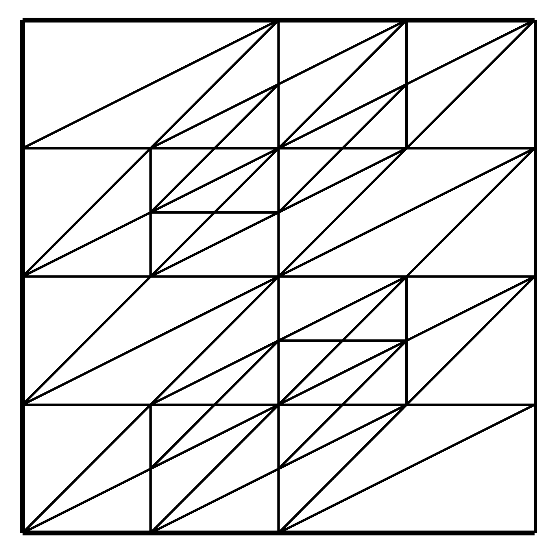 Figure 1
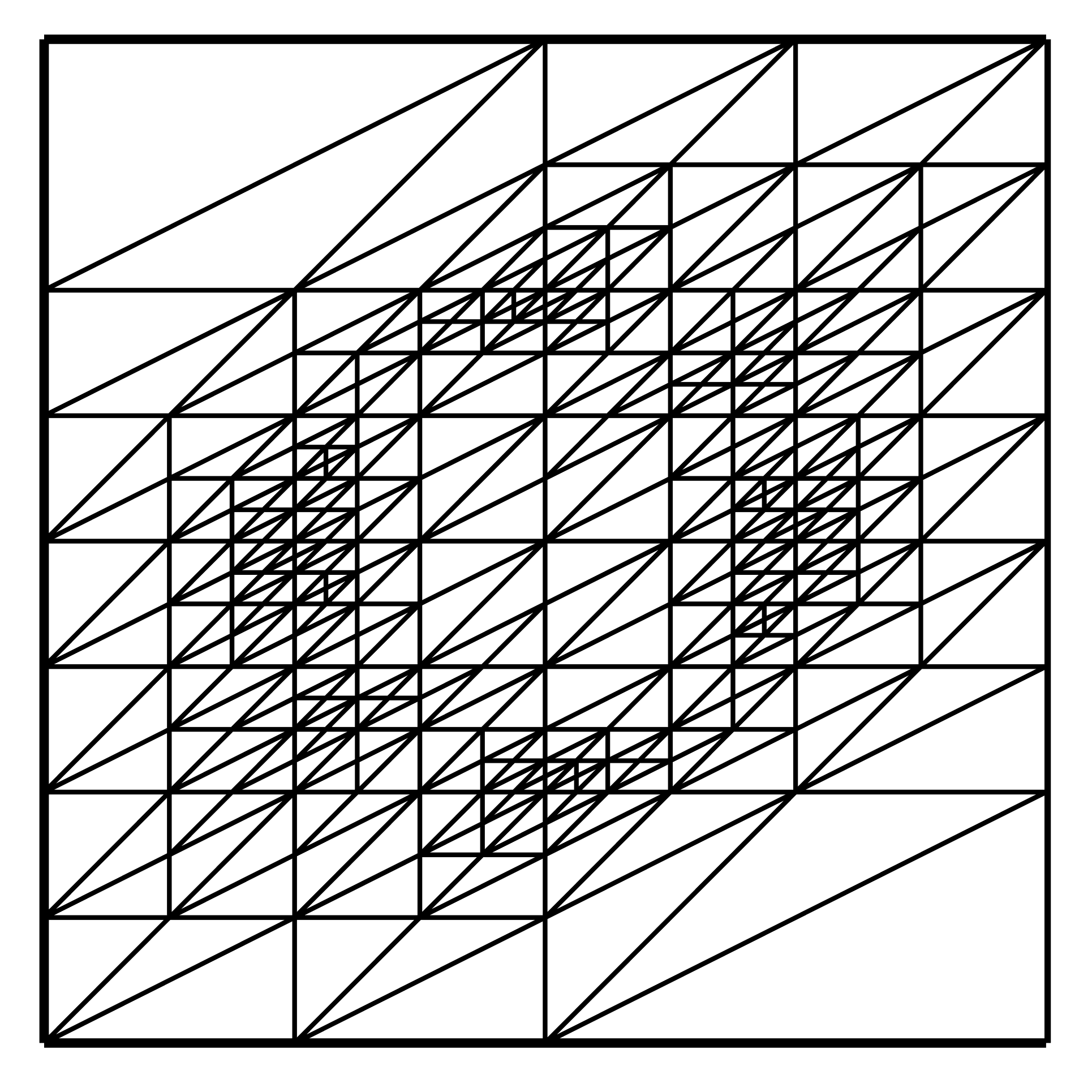 Figure 2
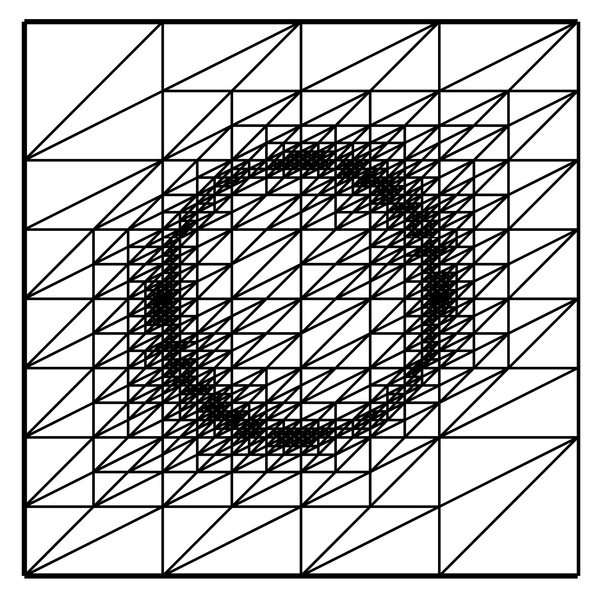 Figure 3
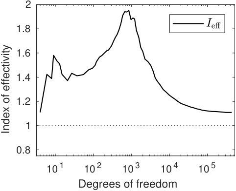 Figure 4
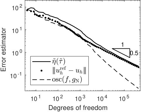 Figure 5
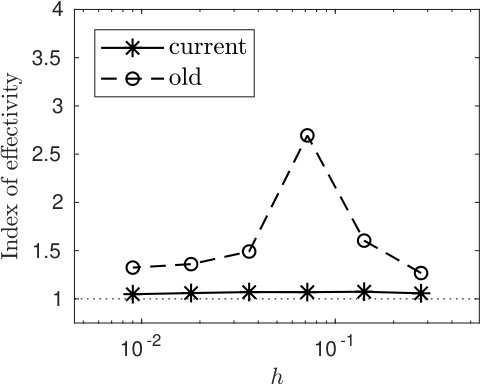 Figure 6
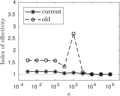 Figure 7
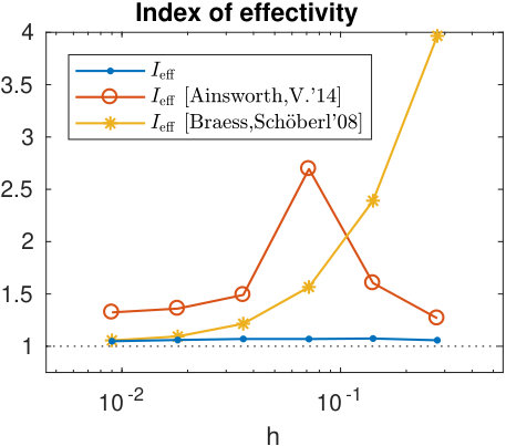 Figure 8
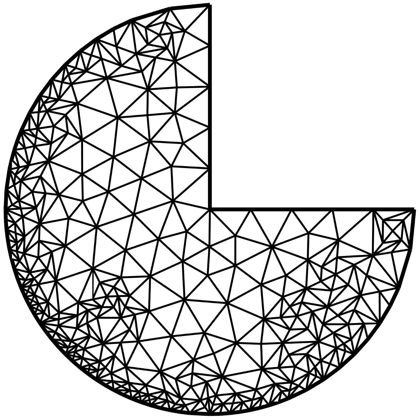 Figure 9
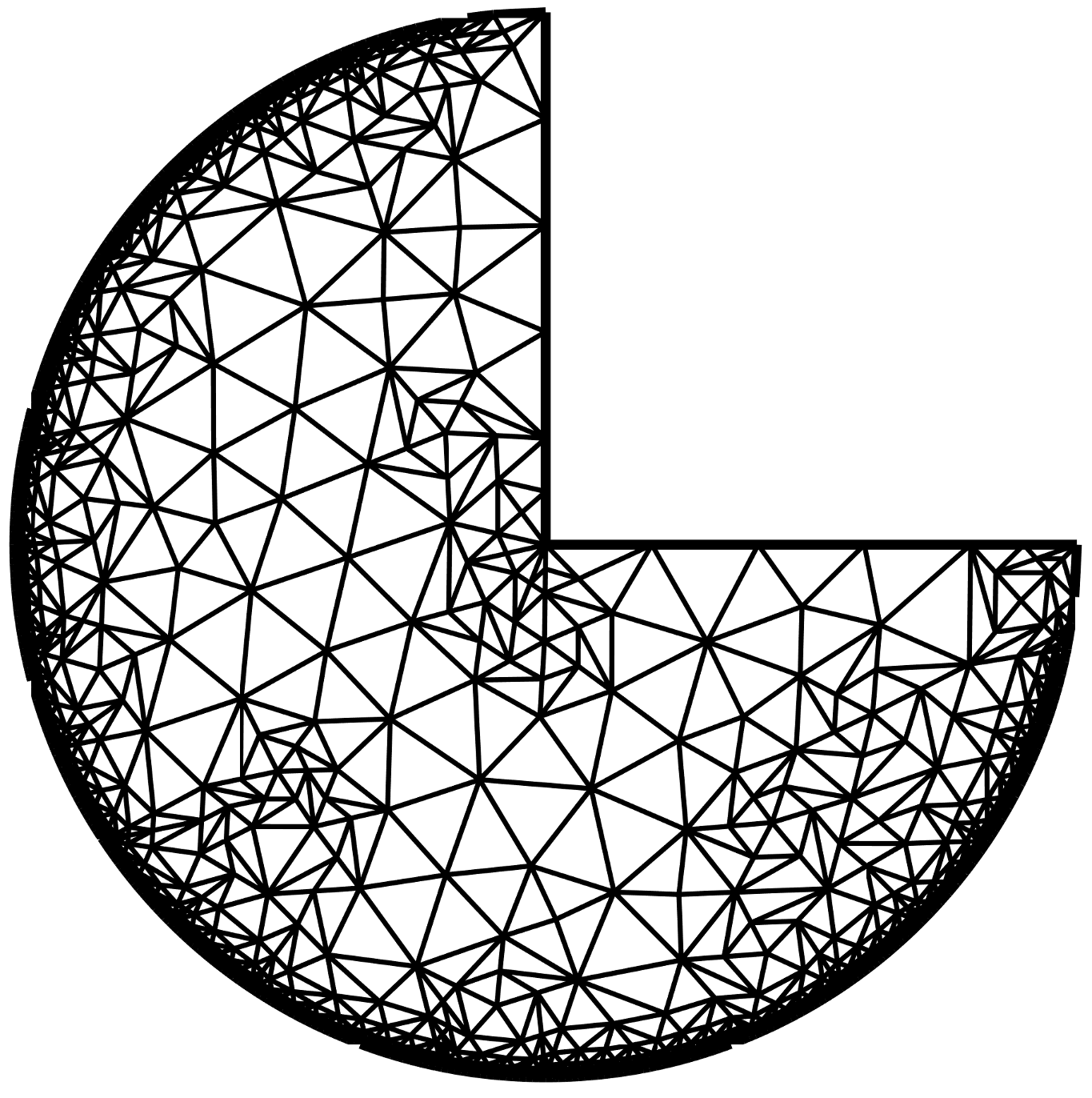 Figure 10
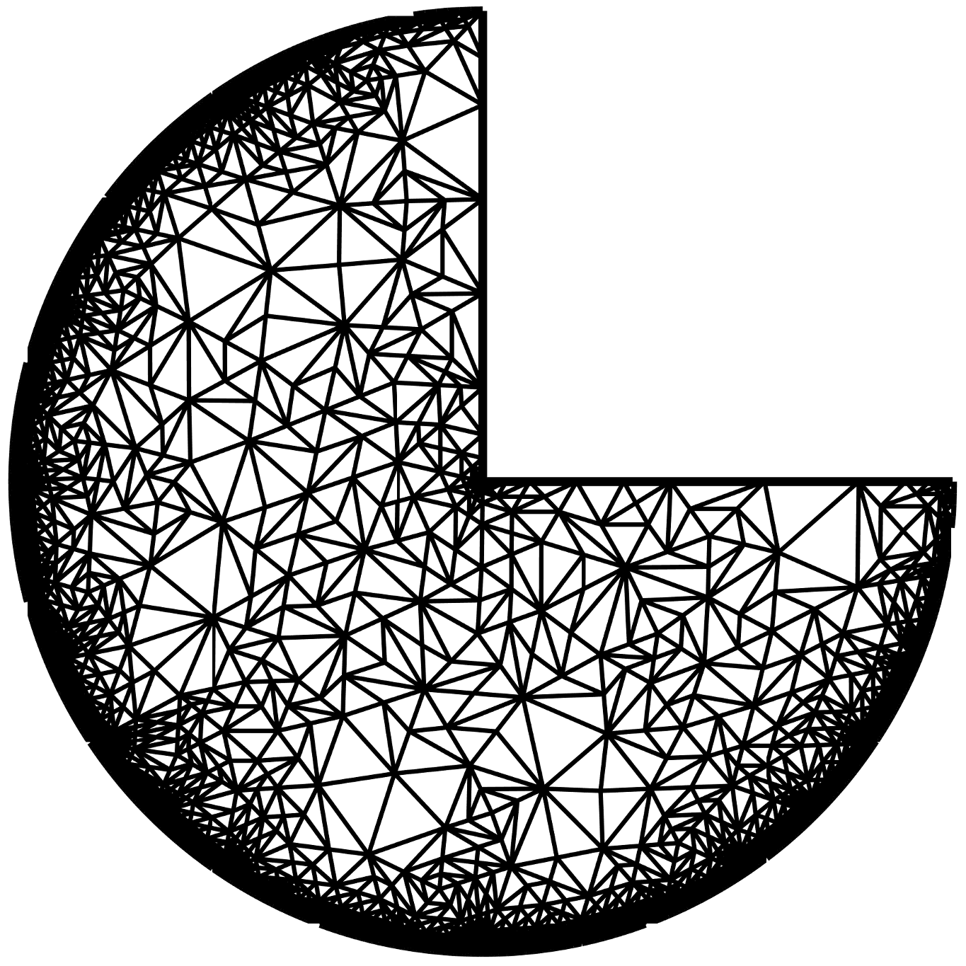 Figure 11
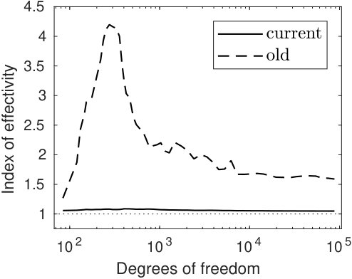 Figure 12
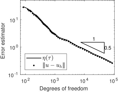 Figure 13
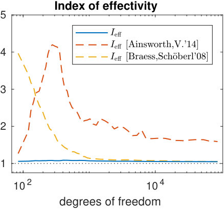 Figure 14
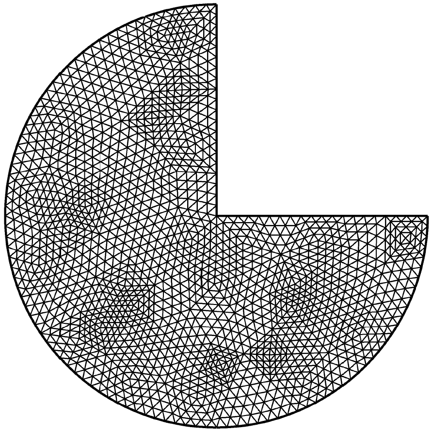 Figure 15
Peer Reviews
No public reviews on file for this paper yet. If you reviewed it on a platform where reviews are public (OpenReview, ICLR, NeurIPS, ICML), you can paste yours below so the community can read it here.
Videos
No videos yet. Explain this paper in a talk, walkthrough, or lecture? Add one.
A Simple Approach to Reliable and Robust A Posteriori Error Estimation
for Singularly Perturbed Problems
Mark Ainsworth
Division of Applied Mathematics, Brown University, 182 George St, Providence, RI 02912, USA and Computer Science and Mathematics Division, Oak Ridge National Laboratory, Oak Ridge, TN 37831, USA, [email protected]
Tomáš Vejchodský T. Vejchodský acknowledges the support of the Czech Science Foundation, project no. 18-09628S, and the institutional support RVO 67985840.
Institute of Mathematics, Czech Academy of Sciences, Žitná 25, CZ-115 67 Prague 1, Czech Republic, [email protected]
Abstract
A simple flux reconstruction for finite element solutions of reaction-diffusion problems is shown to yield fully computable upper bounds on the energy norm of error in an approximation of singularly perturbed reaction-diffusion problem. The flux reconstruction is based on simple, independent post-processing operations over patches of elements in conjunction with standard Raviart–Thomas vector fields and gives upper bounds even in cases where Galerkin orthogonality might be violated. If Galerkin orthogonality holds, we prove that the corresponding local error indicators are locally efficient and robust with respect to any mesh size and any size of the reaction coefficient, including the singularly perturbed limit.
Keywords: finite element analysis, robust a posteriori error estimate, singularly perturbed problems, flux reconstruction
MSC: 65N15, 65N30, 65J15
1 Introduction
This paper is concerned with developing fully computable bounds for the error in the finite element approximation of the following linear reaction-diffusion problem
[TABLE]
where the domain , , is a polytope and denotes the unit outward normal vector on the boundary . Here, the portions and of the boundary are open, disjoint and satisfy . For simplicity, we assume that the data and and that the reaction coefficient is piecewise constant. The problem has a unique solution provided that either has a positive measure or is not identically zero.
Given a conforming approximation of the true solution of problem (1), we present a novel a posteriori error estimator for the energy norm of the error . The estimator is rather easy to evaluate (via a fast element by element algorithm) and provides a guaranteed upper bound on the true error measured in the energy norm. In the case where is the Galerkin finite element approximation of , we prove that the estimator is locally efficient and provides an upper bound which does not degenerate in the singularly perturbed limit (i.e. when ).
This error estimator is evaluated using a reconstructed flux. In contrast to our previous work [1, 3, 4], the reconstructed flux is obtained by solving small local problems on patches of elements by Raviart–Thomas finite elements. This approach is technically simpler and yields a more accurate error estimator.
The idea of the flux reconstruction by solving small problems on patches comes from [6]. It can be seen as approximate minimization of the error bound using an overlapped domain decomposition method with subdomains chosen as patches of elements. Local minimization problems on these patches have equilibration constraints and are solved by by mixed finite elements. Our result can be seen as a robust generalization of this idea to reaction-diffusion problems.
The general idea of flux reconstructions, however, dates back to the method of hypercircle [26, 30] and later to [5, 15, 17, 20, 35]. In the last two decades it was vastly developed, see e.g. [1, 8, 14, 21, 25, 27] and references there in. Interestingly, error estimates based on flux reconstructions can be utilized to estimate various components of the error such as the discretization, iteration, and algebraic errors [10, 12, 16, 23]. This enables us to adaptively equilibrate all components of the error and develop algorithms that do not perform excessive iterations of linear and nonlinear solvers in cases when the iteration and algebraic errors are already on the level of the discretization error.
The first robust, reliable, and locally efficient a posteriori error estimate for problem (1) was derived by Verfürth in [33, 32]. Locally efficient and robust guaranteed error bounds for the vertex-centred finite volume discretization of (1) were proposed in [9]. Robust reliability estimate for singularly perturbed problem on anisotropic meshes is proved in [18]. A similar result for a guaranteed and fully computable error bound is provided in [19]. An interesting alternative idea for guaranteed upper bounds for reaction-diffusion problems was recently published in [24]. Preprint [29] proofs robustness of a simple a posteriori error estimator, however their approach considerably differs from the one presented below due to equilibration of fluxes even if the reaction term dominates and due to the presence of weights in the estimator.
The rest of the paper is organized as follows. Section 2 briefly introduces the finite element approximation of problem (1) and the corresponding notation. Section 3 defines the a posteriori error estimator and proves that it is the guaranteed upper bound on the error. Section 4 introduces flux reconstruction based on local minimization problems and Sections 5 and 6 define two auxiliary flux reconstructions that are used in Section 7 to prove the robust local efficiency of the proposed error indicators. Section 8 proposes alternative flux reconstruction that does not require equilibration condition. Section 9 provides a couple of numerical examples and Section 10 draws the conclusions.
2 Model Problem and Its Discretization
2.1 Partitions
Let be a family of partitionings of the domain into simplicial elements. The intersection of each distinct pair of elements in a given partition is assumed to consist of a single common vertex or a single common facet of both elements. The diameter and inradius of an element are denoted by and , respectively. The family is assumed to be regular in the sense that there exists a constant such that
[TABLE]
This assumption permits meshes in which the elements are locally refined such as might arise from an adaptive refinement algorithm. The patch consisting of an element and those elements in sharing at least one common point with is defined by
[TABLE]
The regularity condition (2) means that the number of elements in any patch is uniformly bounded over the family , as is the number of patches containing a particular element. Further, condition (2) implies the following local quasi-uniformity and shape regularity properties: there exist constants and such that for all elements , all , and all estimates and hold.
Here, and throughout, we adopt the convention whereby the symbol is used to denote a generic constant throughout the paper, whose actual numerical value can differ in different occurrences, but it is always independent of and any mesh-size.
The notation and is used to denote the scalar product and norm over a subset , and we omit the subscript in the case when . The -orthogonal projector onto the space of affine functions over element is denoted by , whist is used to denote the concatenation of the elementwise projections , i.e. for all . Similarly, for a facet , denotes the -orthogonal projector, and denotes the concatenation of the facetwise projections : for all facets .
2.2 Assumptions on the Reaction Coefficient
For simplicity, we shall assume that the reaction coefficient is constant on every element over the entire set of partitions in and we denote by its constant value in . Moreover, we shall assume that the reaction coefficient varies slowly between neighbouring elements in the sense that that there exists a constant such that the following condition holds for all triangulations and all elements :
[TABLE]
We state, without proof, some elementary consequences of the above assumption:
Lemma 1**.**
Suppose that condition (4) holds. Then
if , then on the patch ; 2. 2.
if , then on the patch ; 3. 3.
there exists a constant such that for all , all , if , then
[TABLE]
for all ; 4. 4.
there exists a constant such that for all , all , and all elements ,
[TABLE]
The quantity appears extensively throughout the paper and we shall adopt the convention whereby
[TABLE]
2.3 Finite Element Discretization
The weak formulation of problem (1) reads: find such that
[TABLE]
where and are defined by
[TABLE]
It will be useful to introduce local counterparts of these forms
[TABLE]
The associated global and local energy norms and are defined by and , respectively.
Let , where is the space of affine functions on , then the finite element approximation of (1) is defined by
[TABLE]
3 A Posteriori Error Estimator
Every partition can be split into disjoint subsets and . Let be any vector field satisfying the conditions
[TABLE]
Let in , in , and on , then the local error indicator over an element is defined to be
[TABLE]
Observe that and vanish if and that the second and the third term is taken to be zero on such elements. The error estimator is then defined by
[TABLE]
where the oscillation term is given by
[TABLE]
and the constants
[TABLE]
arose in the corrigendum of [4, Lemma 1].
The following result, based on [4, Lemma 2], shows that the estimator provides an upper bound on the error:
Theorem 2**.**
Let be arbitrary. If satisfies equilibration conditions (8)–(9) then
[TABLE]
Proof.
The weak formulation (6) and the divergence theorem yield identity
[TABLE]
for all . The last two terms are estimated in the same way as in the proof of [4, Lemma 2]:
[TABLE]
For elements we bound
[TABLE]
where the trace inequality [4, Lemma 1] is employed.
Due to equilibration conditions (8)–(9), we arrive at
[TABLE]
Cauchy–Schwarz inequality, notation (11), and choice finish the proof. ∎
It will not have escaped the reader’s notice that nothing in the above argument relies on being a finite element approximation. Consequently, the upper bound presented in Theorem 2 holds true for arbitrary conforming approximation . However, the local efficiency and robustness results proved in Theorem 11 will require to be a Galerkin finite element approximation exactly satisfying the condition (7).
4 Flux Reconstruction by Patchwise Minimization
Let denote the nodes in the partition . In particular, given a node , the subset consists of elements that touch the node, while consists of facets on the Neumann boundary which touch the node .
The flux reconstructions used in the current work are constructed over patch . Specifically, let
[TABLE]
where , denotes the unit outward facing normal vector on the boundary of the patch , and is the standard Raviart–Thomas space.
Let denote the minimizer of the quadratic functional
[TABLE]
over satisfying constraints
[TABLE]
where is the usual piecewise affine and continuous hat function satisfying for all nodes , , , , is the element adjacent to the facet , , and stands for piecewise constant function over facets defined as for all facets such that .
The minimizer of (18) satisfying constraints (19)–(20) could, equally well, be characterised as the unique solution of the following problem: Find and Lagrange multipliers and satisfying
[TABLE]
for all and
[TABLE]
where and are spaces of discontinuous and piecewise affine functions over and , respectively.
The condition in definition (17) imposed on the facets means that can be extended by zero onto thereby obtaining a vector field in , which we again denote by . With this convention in place, the reconstructed flux is taken to be the sum
[TABLE]
The resulting globally defined vector field can be used in (12) to obtain an upper bound on the energy norm of the error, because it satisfies the equilibration conditions as stated in the following lemma.
Lemma 3**.**
*Reconstructed flux given by (24) satisfies equilibration conditions (8)–(9). *
Proof.
Let . Equality (22), definition (24), and partition of unity yield
[TABLE]
for all . Since , equilibration condition (8) follows.
Similarly, given a facet , the equality (23) implies
[TABLE]
for all . Equilibration condition (9) then follows, because . ∎
The next two sections are concerned with showing that reconstructed flux defined in (24) yields locally efficient and robust error indicators. The main idea used in the proof is based on comparing with two judiciously chosen flux reconstructions and . Each of these reconstructions is defined in the neighbourhood of the element , see (3). While the flux reconstruction is based on equilibrated interface fluxes introduced in [1] and analysed in [4], the second reconstruction is new.
5 The First Auxiliary Flux Reconstruction
In this section we introduce the auxiliary flux reconstruction and prove its properties. This flux reconstruction is based on equilibrated interface fluxes. If is the Galerkin solution given by (7) then results of [2] guarantee the existence of interface fluxes satisfying for all elements the following properties
[TABLE]
and equilibration condition
[TABLE]
where stands for the set of vertices of . These fluxes do not yield robust a posteriori error estimators for large values of the reaction coefficient , as it was shown in [1]. However, we will use them only in elements where .
Below, we will utilize two estimates from [4]. First, quantity defined on for all elements satisfies
[TABLE]
see [4, estimate (31)]. Second, residual is bounded as
[TABLE]
see [4, estimate (29)] and also [1, Lemma 5].
The definition of the first auxiliary flux reconstruction proceeds as follows. If an element is such that , then we define
[TABLE]
where is given piecewise as
[TABLE]
and vector fields are determined by the following lemma.
Lemma 4**.**
Let satisfies (7). Let be an element and let be its vertex. Then there exists such that
[TABLE]
and
[TABLE]
Proof.
To establish the existence and uniqueness of we recall [7] that is unisolvent with respect to the degrees of freedom defined by
[TABLE]
and
[TABLE]
Observing that is surjective, we may rewrite the former set of degrees of freedom in the equivalent form
[TABLE]
which, on integrating by parts and using the second set of degrees of freedom, shows that is unisolvent with respect to the degrees of freedom defined by (34) augmented with the following
[TABLE]
Since the data in conditions (32) belong to and since the equilibration condition (27) implies the following compatibility condition
[TABLE]
we deduce that exists and is unique. ∎
The following lemma shows that vector fields lie in .
Lemma 5**.**
Let satisfies (7). Let be a vertex and let be defined by (31). Then and on facets .
Proof.
The fact that follows from the continuity of its normal components over element interfaces. Indeed, if for elements is an interior facet then
[TABLE]
by (26). Similarly, we verify the boundary conditions on required in (17). Clearly, on facets , because on , and on facets by (25). ∎
An interesting consequence of Lemma 5 and identity (33) is that
[TABLE]
The vanishing normal components of on exterior facets guarantee that can be extended by zero and as such belongs to . Consequently, defined in (30) lies in as well. The following lemma shows that satisfies equilibration conditions (8)–(9).
Lemma 6**.**
Let satisfies (7). Let be a fixed element and let be defined by (30). Then
[TABLE]
Proof.
To prove (36), we use definitions (33) and (31) to find that
[TABLE]
holds in . This identity together with the partition of unity , definition (30), and properties of the projection yields
[TABLE]
in .
To prove (37), we consider to be an element adjacent to the Neumann boundary and to be its facet. On this we clearly have
[TABLE]
by (30), (31), (32), (25), and the fact that . Here, stands for the set of vertices of the facet . ∎
Now, we formulate and prove the main result of this section. For an element , we introduce neighbourhood , where is given by (3).
Theorem 7**.**
Let be an element where . Let be its vertex and let be defined by (31). Then
[TABLE]
Proof.
Let and be an element. By (33), the quantity satisfies
[TABLE]
where was introduced above (29). Consequently,
[TABLE]
Now, boundary conditions (32) imply
[TABLE]
and
[TABLE]
where stands for the facet of opposite to the vertex . Since quantity is a norm in the finite dimensional space , we can use the scaling argument
[TABLE]
Thus, using , inequalities (41) and (43), we obtain
[TABLE]
Hence, estimates (29) and (28) applied in (44) yield
[TABLE]
Finally, the bound (39) follows by using the local quasi-uniformity of the mesh. ∎
6 The Second Auxiliary Flux Reconstruction
For elements , where , we define the second auxiliary flux reconstruction as
[TABLE]
where
[TABLE]
and is the -orthogonal projection of onto the space of affine functions on . Note that is supported in and that it is continuous. To simplify the notation we introduce piecewise linear and discontinuous function in the patch by the rule
[TABLE]
For completeness, we define in those patches , where for all .
It is clear that for all and that on facets . Thus can be extended by zero such that and consequently .
Lemma 8**.**
Let be arbitrary. Let be an element such that . Let be its vertex and let be defined by (46). Then
[TABLE]
holds for all .
Proof.
Let be fixed. Recall that Lemma 1 implies , and . The inverse inequality yields
[TABLE]
Similarly,
[TABLE]
where estimate (48) and the fact that were used. Consequently, using bound and triangle inequality, we obtain
[TABLE]
where we employ (29). ∎
Lemma 9**.**
Let be arbitrary. Let be an element such that . Let be its vertex and let be a facet on adjacent to an element . Then
[TABLE]
Proof.
Using the definition (46) of , properties of projection and hat function , we obtain
[TABLE]
To bound this norm, we consider a special test function. We define function on the boundary as on and on , where is a bubble function defined on the facet . Then we introduce minimum energy extension to the interior of satisfying , on , and for all , see [1, Section 3.1]. Extending further by zero to the rest of the domain , we have .
Using as a test function in (6) together with identity , we derive
[TABLE]
Since and is a norm in , we use the equivalence of norms in the finite dimensional space to get
[TABLE]
This estimate together with identity (51), Cauchy–Schwarz inequality, inverse inequality, and bound provided by assumption (4) yields
[TABLE]
Here, the energy norm is bounded by [1, Lemma 4] as
[TABLE]
and norm by using the equivalence of norms in as
[TABLE]
Finally, using these bounds, inequalities and , and estimate (29) in (52), we obtain
[TABLE]
This estimate and (50) finish the proof. ∎
7 Efficiency of Patchwise Minimizations
We first formulate a lemma stating that error indicators can be bounded by the value of the quadratic functional .
Lemma 10**.**
Let be arbitrary. Let stand for the dimension. Let error indicators be defined by (10). Let reconstructed flux given by (24) satisfy equilibration conditions (8)–(9) and let its local components be in . Then
[TABLE]
Proof.
Let simplex be fixed. Since there is facets on the boundary of , we can bound by Cauchy–Schwarz inequality as
[TABLE]
Using the partition of unity , definition of , definition (24) of , and Cauchy–Schwarz inequality, we obtain
[TABLE]
Similarly, we estimate
[TABLE]
and for facets
[TABLE]
Statement (53) now follows by a combination of these estimates.
If then bound (53) is easy to verify, because of identity and estimate (54). ∎
Note that this lemma holds true for any flux given by (24). Its local components are not required to minimize the quadratic functional defined in (18).
The following theorem presents the main result of this paper. It states the efficiency and robustness of error indicators computed by (10) from the patchwise flux reconstruction defined in (24). To formulate it, we introduce the union of facets in the triangulation that lie on and have at least one common point with , i.e., .
Theorem 11**.**
Let be the weak solution (6) and let be its Galerkin approximation satisfying (7). Let flux reconstruction be given by (24) and let its local components solve local problems (21)–(23). Then there exists a constant independent of reaction coefficient and any mesh size such that the local efficiency estimate
[TABLE]
holds true for all elements .
Proof.
We consider two cases. First, let be such that . Since minimizes the functional , both and satisfy constraints (19)–(20), and fluxes satisfy (35), we obtain from (53) the estimate
[TABLE]
Applying Theorem 7 in this inequality immediately yields
[TABLE]
Second, let be such that . By assumption (4), the reaction coefficient satisfies for all elements . Since and is the minimizer of , the inequality (53) yields
[TABLE]
Estimates (47) and (49) then give
[TABLE]
Assumption (4) and a combination of (56) and (57) finishes the proof. ∎
The oscillation term is not standard, however, as well as the other oscillation terms in (55) it is of higher order than the error and does not spoil the robust local efficiency result.
8 Avoiding Equilibration
Theorem 2 requires the flux to satisfy equilibration conditions (8)–(9). Therefore, the local minimization problems (18) is constrained by (19)–(20). However, in practical computations constraints (19)–(20) are often not satisfied exactly due to round-off errors. Consequently, assumptions of Theorem 2 are not valid and error estimator is not guaranteed to provide the upper bound on the error. This problem can be avoided by introducing Friedrichs–Poincaré and trace inequalities and two additional parameters in the definition of the estimator.
Given arbitrary flux , we define modified local error indicators
[TABLE]
where small parameter replaces the zero value of in a sense and small parameter has a similar meaning. Notice that differs from only for elements .
The modified error estimator is then defined as
[TABLE]
where and are constants from Friedrichs–Poincaré and trace inequalities
[TABLE]
The following theorem presents a modification of Theorem 2 that avoids the equilibration conditions (8)–(9).
Theorem 12**.**
Let and be arbitrary. Then
[TABLE]
for all and .
Proof.
Using identity (13) and estimates (14)–(16), we arrive at
[TABLE]
Using Cauchy–Schwarz inequality
[TABLE]
we obtain
[TABLE]
Friedrichs–Poincaré and trace inequalities (60), notation (59), and choice finish the proof. ∎
Constants and should be small. Ideally so small that . In this case the influence of Friedrichs–Poincaré and trace constants and on the value of the error bound (61) is negligible. In the case of pure Dirichlet boundary conditions, i.e., , the parameter is not needed and estimate (61) holds with . In case everywhere in the set is empty and parameters , and constants , are not needed. Estimate (61) then holds with and local error indicators (10) and (58) coincide. However, if vanishes at some parts of and constants and are needed, then they can be computed analytically in some special cases and numerically, in general. Even their guaranteed numerical bounds are available, see e.g. [28, 31].
Since Theorem 12 does not require any equilibration condition, the patchwise flux reconstruction procedure simplifies. Modified fluxes minimize the quadratic functional
[TABLE]
over the space , where is the union of the facets belonging to and piecewise constant parameters and are given by
[TABLE]
for all elements and all facets , where we recall that denotes the element adjacent to the facet .
The minimizer of (62) could, equally well, be characterised as the unique solution of the following problem:
[TABLE]
for all . Note that the large values and play here the role of penalty parameters to impose constraints (19)–(20) and (22)–(23) in a weak sense. Consequently, the difference between and is small in practical computations.
Summing up fluxes as in Section 4 results in a modified reconstructed flux
[TABLE]
that can be directly used in Theorem 12 to obtain a guaranteed upper bound on the error.
The modified reconstructed flux is locally efficient and robust as it is stated in the following corollary.
Corollary 13**.**
Let be the weak solution (6) and let be its Galerkin approximation satisfying (7). Let flux reconstruction be given by (65) and let its local components solve local problems (64). Then there exists a constant independent of reaction coefficient and any mesh size such that the local efficiency estimate
[TABLE]
holds true for all elements .
Proof.
The proof follows the same lines as the proof of Theorem 11. In particular, we use the fact that
[TABLE]
∎
9 Numerical Examples
Example 1
In this example, we consider problem (1) in a domain with reentrant corner: , where and are standard polar coordinates, see Figure 1 (left). The boundary conditions are homogeneous Dirichlet only, i.e., and . The reaction coefficient is assumed positive, constant in , and its specific values are provided below. Choosing the right-hand side as , the exact solution is explicitly given by
[TABLE]
where stands for the modified Bessel function of the first kind. This solution exhibits singularity at the origin and a boundary layer at for large values of .
We first compute the finite element solution (7) using the mesh shown in Figure 1 (right) for , . For each value of we compute flux reconstruction (24) by solving local problems (21)–(23) and evaluate the error estimator given by (11). Note that since and , the procedure considerably simplifies. The set is empty, equilibration conditions (8)–(9) do not apply as well as constraints (22)–(23). Reconstructed fluxes and given by (24) and (65), respectively, are identical and for all . In particular constants , , , and are not needed.
Figure 2 (left) presents the index of effectivity
[TABLE]
for the chosen values of . All values of are above 1 confirming that is the guaranteed upper bound on the error. On the other hand they are not far from 1 in the whole range of values of showing the robust efficiency. All these indices of effectivity are below 1.12, which illustrates high accuracy of computed error estimators. For comparison, we also present indices of effectivity for the error estimator proposed in our previous work [4], see the dashed lines in Figure 2. Its accuracy legs behind the current approach.
To illustrate the robustness with respect to the mesh size, we also solve this problem on a sequence of uniformly refined meshes for a fixed value and plot the resulting indices of effectivity in Figure 2 (right). In this case we observe robust efficiency and high accuracy as well.
Error indicators given in (10) can be utilized for adaptive mesh refinement and error estimator for a guaranteed stopping criterion. We use the standard adaptive algorithm: SOLVE – ESTIMATE – STOP – MARK – REFINE. Given an initial mesh, the SOLVE step computes the finite element solution by (7), the ESTIMATE step evaluates the flux reconstruction defined by (24) and error indicators introduced in (10). In the STOP step, the error estimator given by (11) is computed and the algorithm is stopped if (and consequently the error ) is below the required tolerance. In the MARK step, the Dörfler strategy [11] is used to mark elements, where indicate large error. Finally, the longest edge bisection algorithm [22, 34] is applied in the REFINE step to refine the marked elements and create a new mesh.
Several examples of adaptively refined meshes are provided in Figure 3. The optimal speed of convergence of both the error and error estimator during the adaptive algorithm is presented in Figure 4 (left). Figure 4 (right) shows corresponding indices of effectivity. They are all above and quite close to 1, confirming the robust efficiency of the error estimator even on highly graded meshes.
Example 2
This example illustrates the behaviour of the proposed error estimator for a discontinuous right-hand side , piecewise constant reaction coefficient , and homogeneous Neumann boundary conditions. We consider problem (1) in a square with and on . Right-hand side equals to in the disc , where is the distance from the origin, and it vanishes elsewhere. The exact solution of this problem is not known, but for large it is supposed to be close to the characteristic function of the disc with a steep interior layer close to the boundary of . Since the exact solution is not known, we approximate the true error by , where the reference solution is computed by finite elements of order 5 on the same mesh as .
We choose and use the modified flux reconstruction (65) and the modified error estimator (59). Since is a square, we can compute the Friedrichs–Poincaré and trace constants analytically. We use and . Parameters and are chosen as square roots of the machine epsilon: .
We solve this problem by the adaptive algorithm described above starting with a mesh with two triangles. This setting does not satisfy assumptions listed in Subsection 2.2, because discontinuities in are not compatible with the mesh. Therefore, for the purpose of computation, we use the value of in the centroid of each element as the constant value in the element. In this way we construct certain approximate solution and the corresponding error estimator, which is guaranteed by Theorem 12 to be above the true error. The obtained indices of effectivity show robust and efficient performance of the estimator even in this case.
Figure 5 (left) shows the energy norm of the approximate error , the computed error bound , and the oscillation term during the adaptive process. Figure 5 (right) presents the corresponding indices of effectivity . We may observe that the error bound is really above the error and that the error estimator estimates it robustly on all meshes. The oscillation term is of comparable size as the error at the beginning of the adaptive process, which leads to higher values of the index of effectivity. However, starting from meshes with around degrees of freedom the interior layer is well resolved, the oscillation term decreases faster than the error, and the index of effectivity decreases towards one. For illustration we present three adaptively refined meshes in Figure 6.
10 Conclusions
In this paper we present an a posteriori error estimator that is fully computable and provides a locally efficient upper bound on the energy norm of the error. This error estimator can be computed by a fast and easily parallelizable algorithm by solving small and independent problems on patches of elements. We proved its robustness both with respect to the mesh size and the reaction coefficient . We demonstrated by numerical examples that the corresponding local error indicators can be successfully used in the standard adaptive algorithm to guide the mesh adaptation and that the error estimator provides sharp results on rough, fine, and adaptively refined meshes as well as in the singularly perturbed case when is large.
Further research questions about this error estimator may include its robustness for higher order finite element approximations [29] and its possible modifications to guarantee robustness on anisotropically refined meshes.
The proposed flux reconstruction can be used not only for the presented reaction-diffusion problems, but also for related eigenvalue problems. It was recently shown [31] that any flux reconstruction for boundary value problems can be directly used in the Lehmann–Goerisch method for guaranteed bounds on eigenvalues.
The reference list from the paper itself. Each links out to its DOI / PubMed record.
- 1[1] Ainsworth, M. and Babuška, I.: Reliable and robust a posteriori error estimating for singularly perturbed reaction-diffusion problems. SIAM J. Numer. Anal. 36 (1999), 331–353 (electronic).
- 2[2] Ainsworth, M. and Oden, J.T.: A posteriori error estimation in finite element analysis . Pure and Applied Mathematics (New York), Wiley-Interscience [John Wiley & Sons], New York, 2000.
- 3[3] Ainsworth, M. and Vejchodský, T.: Fully computable robust a posteriori error bounds for singularly perturbed reaction–diffusion problems. Numer. Math. 119 (2011), 219–243.
- 4[4] Ainsworth, M. and Vejchodský, T.: Robust error bounds for finite element approximation of reaction-diffusion problems with non-constant reaction coefficient in arbitrary space dimension. Comput. Methods Appl. Mech. Engrg. 281 (2014), 184–199.
- 5[5] Aubin, J.P. and Burchard, H.G.: Some aspects of the method of the hypercircle applied to elliptic variational problems. In: Numerical Solution of Partial Differential Equations, II (SYNSPADE 1970) (Proc. Sympos., Univ. of Maryland, College Park, Md., 1970) , pp. 1–67. Academic Press, New York, 1971.
- 6[6] Braess, D. and Schöberl, J.: Equilibrated residual error estimator for edge elements. Math. Comp. 77 (2008), 651–672.
- 7[7] Brezzi, F. and Fortin, M.: Mixed and hybrid finite element methods . Springer-Verlag, New York, 1991.
- 8[8] Cai, Z. and Zhang, S.: Flux recovery and a posteriori error estimators: conforming elements for scalar elliptic equations. SIAM J. Numer. Anal. 48 (2010), 578–602.