Uniformly convergent expansions for the generalized hypergeometric functions of the Bessel and Kummer types
Jose L.Lopez, Pedro J.Pagola, Dmitrii B.Karp

TL;DR
This paper develops uniformly convergent expansions for generalized hypergeometric functions of Bessel and Kummer types, providing explicit error bounds and numerical validation across complex domains.
Contribution
It introduces new uniform convergent expansions for hypergeometric functions in terms of Bessel, confluent hypergeometric, trigonometric, exponential, and rational functions.
Findings
Explicit error bounds are provided for all expansions.
Numerical experiments demonstrate the accuracy of the approximations.
The expansions hold uniformly in specified complex domains.
Abstract
We derive a convergent expansion of the generalized hypergeometric function in terms of the Bessel functions that holds uniformly with respect to the argument in any horizontal strip of the complex plane. We further obtain a convergent expansion of the generalized hypergeometric function in terms of the confluent hypergeometric functions that holds uniformly in any right half-plane. For both functions, we make a further step and give convergent expansions in terms of trigonometric, exponential and rational functions that hold uniformly in the same domains. For all four expansions we present explicit error bounds. The accuracy of the approximations is illustrated with some numerical experiments.
Click any figure to enlarge with its caption.
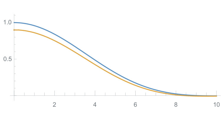 Figure 1
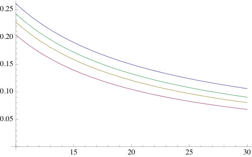 Figure 2
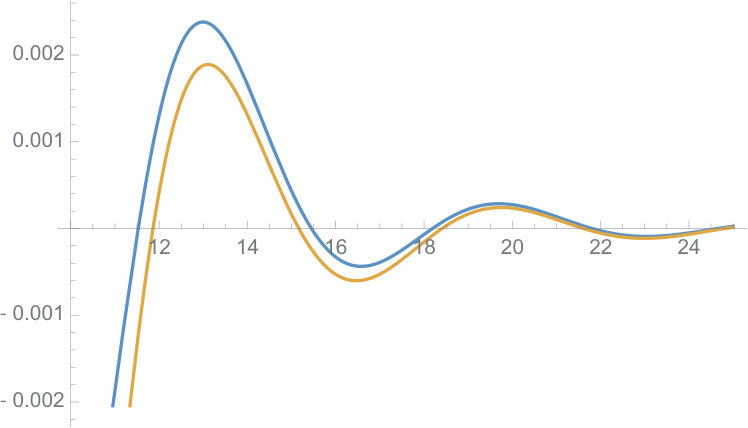 Figure 3
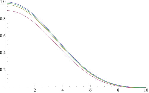 Figure 4
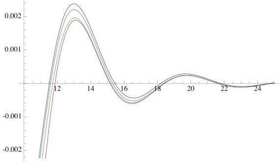 Figure 5
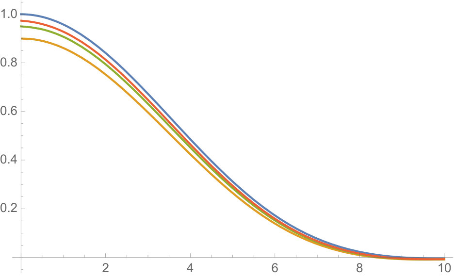 Figure 6
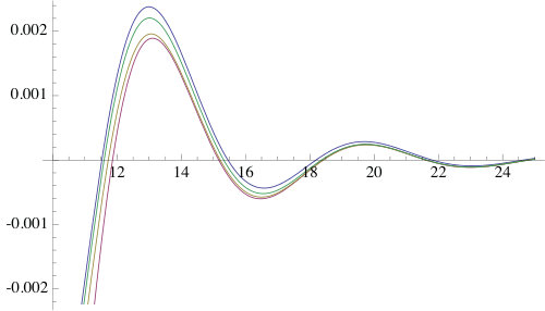 Figure 7
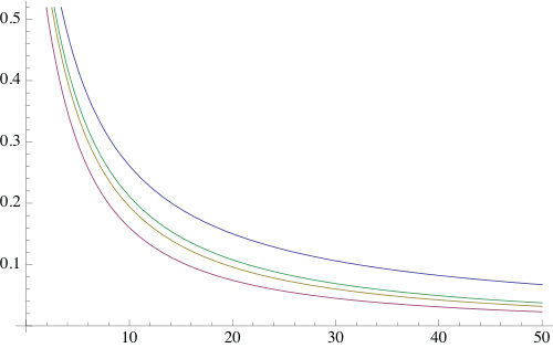 Figure 8
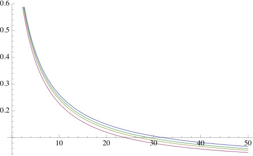 Figure 9
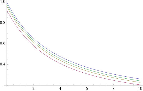 Figure 10
Peer Reviews
No public reviews on file for this paper yet. If you reviewed it on a platform where reviews are public (OpenReview, ICLR, NeurIPS, ICML), you can paste yours below so the community can read it here.
Videos
No videos yet. Explain this paper in a talk, walkthrough, or lecture? Add one.
Taxonomy
TopicsMathematical functions and polynomials · Iterative Methods for Nonlinear Equations · Fractional Differential Equations Solutions
Uniformly convergent expansions for the generalized hypergeometric functions of the Bessel and Kummer types
José L.López∗ , Pedro J.Pagola∗ , Dmitrii B.Karp*†*
* Dpto. de Ingeniería Matemática e Informática,
Universidad Pública de Navarra, Spain
Far Eastern Federal University, Vladivostok, Russia
and Institute of Applied Mathematics FEBRAS*
email: [email protected], [email protected], [email protected]
Abstract
We derive a convergent expansion of the generalized hypergeometric function in terms of the Bessel functions that holds uniformly with respect to the argument in any horizontal strip of the complex plane. We further obtain a convergent expansion of the generalized hypergeometric function in terms of the confluent hypergeometric functions that holds uniformly in any right half-plane. For both functions, we make a further step and give convergent expansions in terms of trigonometric, exponential and rational functions that hold uniformly in the same domains. For all four expansions we present explicit error bounds. The accuracy of the approximations is illustrated with some numerical experiments.
2010 AMS Mathematics Subject Classification: 33C20; 41A58; 41A80.
Keywords & Phrases: generalized hypergeometric function; Bessel function; Kummer function; convergent expansions; uniform expansions.
1 Introduction
A variety of expansions (convergent or asymptotic) of the special functions of mathematical physics can be found in the literature. These expansions have the important property of being given in terms of elementary functions: mostly, positive or negative powers of a certain variable and, sometimes, other elementary functions. However, very often, these expansions are not simultaneously valid for small and large values of . Thus, it would be interesting to derive new convergent expansions in terms of elementary functions that hold uniformly in in a large region of the complex plane containing both small and large values of .
In [5], [6] and [16], the authors derived new uniform convergent expansions of the incomplete gamma functions, the Bessel functions and the confluent hypergeometric functions, respectively, in terms of elementary functions. The starting point of the technique used in [5], [6] and [16] is an appropriate integral representation of these functions. The key idea is the use of the Taylor expansion of a certain factor of the integrand that is independent of the variable , at an appropriate point of the integration interval, and subsequent interchange of sum and integral. The independence of that factor of translates into uniform convergence of the resulting expansion in a large region of the complex plane. The expansions given in [5], [6] and [16] are accompanied by error bounds and numerical experiments showing the accuracy of the approximations.
In this work, we continue that line of investigation by considering the generalized hypergeometric functions and . We view them as functions of the complex variable , and derive new convergent expansions uniformly valid in an unbounded region of the complex plane that contains the point . The generalized hypergeometric function (GHF) is defined by means of the hypergeometric series as (see [1, Section 2.1], [17, Section 5.1], [4, Chapter 12] or [18, eq. (16.2.1)])
[TABLE]
where and , , are parameter vectors and is the Pochhammer’s symbol. In general, does not exist when some . Series (1) converges if and inside the unit disk if . In the latter case, the generalized hypergeometric function is defined outside the unit disk by analytic continuation to the cut plane and the branch defined in this way in the sector , is called the principal branch (or principal value) of .
In the remaining part of this paper we only consider or and , . In the case we assume that . In this case our starting point is the integral representation of originally derived by Kiryakova [15, Chapter 4] and further discussed in [10, eq.(12)] and [11, eq.(28)] which, when combined with the shifting property (8), takes the form:
[TABLE]
where is a particular case of Meijer’s function defined and further explained in (7) below. If we assume that . In this case our starting point is the integral representation of derived in [15, Chapter 4] and further discussed in [10, eq.(11)],
[TABLE]
If the above restrictions on parameters are violated the results of this paper can still be applied by employing the decomposition [11, eq.(31)]
[TABLE]
Indeed, we can always choose large enough to satisfy and .
The power series expansion (1) may be obtained from (2) or (3) by replacing the factor or by its Taylor series at the origin, interchanging series and integral and using the following formula for the moments of the function [11, eq.(16)],
[TABLE]
The Taylor expansions for and converge for , but the convergence is not uniform in . Therefore, expansion (1) is convergent, but not uniformly in as the remainder is unbounded for large .
The asymptotic expansions of and for large can be found in [18, Sec. 16.11]. They are given in terms of formal series expansions in inverse powers of and are asymptotic for large , but the remainders are unbounded for small and then, the expansions are not uniform in .
As an illustration of the uniform approximations that we are going to obtain in this paper (see Theorems 1-4 below), we derive, for example, the following one:
[TABLE]
that approximates the left hand side in any horizontal strip of the complex plane. Note that the limit of the right hand side of (5) as is finite and equals . Figure 1 illustrates the accuracy and the uniform character of the above approximation for real .
In order to derive uniformly convergent expansions of and , we apply the technique proposed in [5], [6] and [16]: we consider the Taylor expansion of the factor at in (2) and (3). This Taylor expansion is convergent for any in the interval of integration and, obviously, it is independent of . After the interchange of the series and the integral, this independence translates into a remainder that may be bounded uniformly with respect to in a large unbounded region of the complex plane that contains the point and that we specify in Theorems 1-4 below.
This paper is organized as follows. In the preliminary Section 2, some properties of the Meijer-Nørlund function and Nørlund’s coefficients needed for later computations are presented and some notation introduced. In Section 3 we consider the integral representation (2) for . In Section 4 we consider the integral representation (3) for . In these two sections we first derive expansions in terms of the Bessel and the confluent hypergeometric functions, respectively. We may consider these expansion as ”natural”, as the Bessel function and the confluent hypergeometric function are the first functions of the respective hierachies. Next, using the known expansions of the Bessel and the confluent hypergeometric functions in terms of elementary functions from [6] and [16], we proceed to derive, for both and , a second expansion in terms of elementary functions. Throughout the paper we use the principal argument .
2 Preliminaries on the Meijer-Nørlund function and Nørlund’s coefficients
We will use the standard notation , and for the sets of natural, integer and complex numbers, respectively; . The size of a vector is typically obvious from the subscript of the corresponding hypergeometric function. Throughout the paper, we will use the shorthand notation for products and sums:
[TABLE]
inequalities like and properties like will be understood element-wise. The symbol stands for the vector with omitted -th component. Given two complex vectors , , we also define
[TABLE]
We will need the basic properties of a particular case of Meijer’s function studied in detail by Nørlund in [19] using a different notation and without mentioning Meijer’s previous work. In [12] we suggested the denomination ”Meijer-Nørlund function” for this function defined by the Mellin-Barnes integral of the form
[TABLE]
We omit the details regarding the choice of the contour as the definition of (the general case of) Meijer’s function can be found in standard text- and reference- books [17, section 5.2], [18, 16.17], [21, 8.2] and [4, Chapter 12]. See also our papers [11, 12, 13]. The following shifting property is straightforward from the definition (7), but nevertheless it is very useful (see [21, 8.2.2.15] or [18, Sec. 16.19, eq. (16.19.2)]):
[TABLE]
Given two complex vectors , and , Nørlund’s coefficients are defined via the generating function [19, eq.(1.33)], [11, eq.(11)] which we present in a split form for further reference:
[TABLE]
where
[TABLE]
and is defined by (6). These coefficients are polynomials symmetric in the components of the vectors and . They can also be defined via the inverse factorial generating function [19, eq.(2.21)]
[TABLE]
As, clearly, , we have (by changing )
[TABLE]
Hence, for any . Nørlund found two different recurrence relations for (one in and one in ). The simplest of them reads [19, eq.(2.7)]
[TABLE]
with the initial values , , . This recurrence was solved by Nørlund [19, eq.(2.11)] as follows:
[TABLE]
where we applied
[TABLE]
Note that the presence of the terms allows extending the above sums to without changing their values. The other recurrence relation for discovered by Nørlund [19, eq.(1.28)] has order in the variable and coefficients polynomial in . Details can be found in [13, section 2.2]. The first three coefficients are given by (see [13, Theorem 3.1] for details):
[TABLE]
[TABLE]
For and and arbitrary explicit expressions for have also been found by Nørlund, see [19, eq.(2.10)]. Defining , we have
[TABLE]
The right hand side here is invariant with respect to the permutation of the elements of . Finally, for we have [13, p.12]
[TABLE]
The following lemma will play an important role in proving the convergence of the expansions considered in the sequel.
Lemma 1**.**
Given two complex vectors and , denote by the real part of the rightmost pole(s) of the function and write for the maximal multiplicity among all poles with the real part . Then for there exists a constant independent of such that
[TABLE]
Proof.
Assume first that . This implies that the rightmost pole(s) of the function coincide with the rightmost pole(s) of the function . Define
[TABLE]
by (9). It follows from the properties of the Meijer-Nørlund function that is analytic in the domain
[TABLE]
for some and . Further, from the asymptotic properties of in the neighborhood of given in [11, Property 5] we conclude that
[TABLE]
where and are as defined in the Lemma. Hence, we are in position to apply [9, Theorem 2] stating that
[TABLE]
Next, assume that . Take large enough to make the real part of the rightmost pole(s) of the function positive and denote this real part , so that and we are in the situation treated above. Hence, using , and we get
[TABLE]
∎
Remark. In some situations below we will need an extended version of inequality (13) valid for all . It is straightforward to see that (13) implies that the inequality
[TABLE]
is true with some positive constant for all and any .
Lemma 2**.**
Suppose and retain their meaning from Lemma 1 and assume further that . Then for the remainder in formula (9) satisfies
[TABLE]
for some constant independent of and .
Proof.
For , and using the previous lemma we have
[TABLE]
Then
[TABLE]
where is the Hurwitz zeta function [18, section 25.11], whose integral representation [18, eq.(25.11.25)] was used in the second equality. Here the constants are independent of . Further,
[TABLE]
The term is bounded by a sum of terms , with , the highest one corresponding to :
[TABLE]
∎
3 Expansions for the Bessel type GHF
3.1 An expansion in terms of Bessel functions
Theorem 1**.**
For with , and , let and be the constants defined in Lemma 1. Then, if , for any we have
[TABLE]
where
[TABLE]
with independent of and . Therefore, (16) converges uniformly with respect to in any horizontal strip with arbitrary .
Proof.
Substituting the expansion (9) into formula (2) and integrating term-wise we get
[TABLE]
where we used the shifting property and the integral evaluation
[TABLE]
valid for when . Expansion (18) can be rewritten in the form (16), in terms of Bessel functions, in view of
[TABLE]
From Lemma 2 we have that
[TABLE]
with independent of and , which is (17). ∎
The following picture illustrates the accuracy and uniform character of approximation (16) for , , and real .
Remark. In view of the first formula in (12), expansion (16) for takes the form
[TABLE]
where . Surprisingly, we could not find the above expansion in [20]. On the other hand, [20, eq.(5.7.8.3)] reads (after some change of notation):
[TABLE]
As we have in the denominator, for small this series converges faster than our expansion. However, this expansion is not uniform in in any unbounded domain.
3.2 An expansion in terms of elementary functions
Theorem 2**.**
For with , and , let and be the constants defined in Lemma 1. Then, if , for any we have
[TABLE]
where and are the following rational functions of :
[TABLE]
The remainder is bounded in the form
[TABLE]
with independent of and . Therefore, for , (19) converges uniformly with respect to in any horizontal strip with arbitrary .
Proof.
From [16, eq.(9)] we have that, for , the Bessel function may be written as
[TABLE]
with and given in (20) and, if , the remainder is bounded as follows:
[TABLE]
with independent of and . Therefore, the remainder is asymptotically equivalent to as uniformly in in any fixed horizontal strip.
Hence, substituting (22) into (18) we obtain (19) with
[TABLE]
with as in Theorem 1. Here we need to choose to make
[TABLE]
converge to zero as . Using the estimates (14) and (23), with we get
[TABLE]
Then, it is sufficient to take to obtain
[TABLE]
with independent of and and (21) follows. ∎
Formula (5) is a particular case of (19) for . The following picture shows some more approximations.
4 Expansions for the GHF of the Kummer type
4.1 An expansion in terms of the Kummer functions
Theorem 3**.**
Given , assume without loss of generality that and suppose that . Suppose further that , and denote by the real part of the rightmost pole(s) of the function and by the maximal multiplicity among all poles with the real part . Then, if , for any we have
[TABLE]
where is the Kummer function of the first kind, and the remainder is bounded in the form
[TABLE]
with independent of and and . Therefore, expansion (24) is uniformly convergent for in any half-plane with arbitrary .
Proof.
Assume without loss of generality that (otherwise just exchange the indices and . The integral representation [10, eq.(11)] of combined with [2, Sec. 16.19, eq. (16.19.2)] and the shifting property (8) gives
[TABLE]
where , . Then, we are in the position to apply expansion (9) to get:
[TABLE]
where
[TABLE]
Now by the shifting property of Nørlund’s coefficients and definition (6) we have
[TABLE]
so that we arrive at expansion (24) with the remainder given by (after termwise integration)
[TABLE]
In view of , we have
[TABLE]
where is defined in the statement of the theorem. Now, if we write for the real part of the rightmost pole(s) of the function and for the maximal multiplicity among all poles with the real part , Lemma 1 yields
[TABLE]
Combining these bounds we obtain
[TABLE]
for some positive constant independent of and , and
[TABLE]
The representation [3, eq.1.3(3)] ( is the Euler-Mascheroni constant)
[TABLE]
valid for all , implies that the sequence is bounded by a constant. Hence by Lemma 2 we get the bound (25). ∎
The following picture illustrates the accuracy and the uniform character of approximation (24) for , , and real .
4.2 An expansion in terms of elementary functions
Theorem 4**.**
Given , assume that and let and have the same meaning as in Theorem 3. Then, for for any we have
[TABLE]
with , and
[TABLE]
[TABLE]
The remainder term is bounded in the form
[TABLE]
with independent of and , . Therefore, expansion (27) is uniformly convergent any half plane with arbitrary .
Proof.
According to [6, (21),(28)] for each , we can write the Kummer function in the form:
[TABLE]
with and defined above. We also have that, for , the remainder is bounded in the form:
[TABLE]
with independent of and and . Therefore, the remainder behaves as as uniformly in in any half-plane of the form , .
Hence, substituting (29) into (24) we obtain (27) with
[TABLE]
Next, we need to choose to make
[TABLE]
converge to zero as .
Assuming that , we can use the estimate (30) with in view of and estimate (14) to get
[TABLE]
Then, it is sufficient to take and we obtain
[TABLE]
with independent of and which implies (28). ∎
The following picture illustrates the accuracy and the uniform character of approximation (27) for , , and real .
5 Acknowledgments
The authors López and Pagola acknowledge the Dirección General de Ciencia y Tecnología (REF. MTM2017-83490-P) for its financial support.
The reference list from the paper itself. Each links out to its DOI / PubMed record.
- 1[1] G.E. Andrews, R. Askey and R. Roy, Special functions , Cambridge University Press, 1999.
- 2[2] R.A. Askey and A.B. Olde Daalhuis, Generalized Hypergeometric Functions and Meijer G-Function, in: NIST Handbook of Mathematical Functions , Cambridge University Press, Cambridge, 2010, pp. 403–418 (Chapter 16).
- 3[3] H. Bateman, A. Erdélyi, Higher transcedental functions, Volume I, Mac Grow Hill Book Company, 1953.
- 4[4] R. Beals and R. Wong, Special Functions and Orthogonal Polynomials , Cambridge Studies in Advanced Mathematics (No. 153), Cambridge University Press, 2016.
- 5[5] B . Bujanda, J.L. López and P.J. Pagola , Convergent expansions of the incomplete gamma functions in terms of elementary functions, Anal. Appl , 1 6 n. 3 (2018) 435-448.
- 6[6] B . Bujanda, J.L. López and P.J. Pagola , Convergent expansions of the confluent hypergeometric functions in terms of elementary functions. Math. Comput. , 2018. DOI:10.1090/mcom/3389.
- 7[7] W. Bühring, Generalized Hypergeometric functions at unit argument, Proc. Am. Math. Soc. , 1 14 n. 1 (1992), 145–153.
- 8[8] J. Bustoz and M.E.H. Ismail, On gamma function inequalities, Math. Comp. 47 (1986), 659–667.