Exponential Convergence and stability of Howards's Policy Improvement Algorithm for Controlled Diffusions
B. Kerimkulov, D. \v{S}i\v{s}ka, {\L}. Szpruch

TL;DR
This paper proves exponential convergence rates and stability for Howard's policy improvement algorithm applied to controlled diffusions, using backward stochastic differential equations to analyze the algorithm's robustness.
Contribution
It establishes the first global convergence rate and stability results for the continuous-time policy improvement algorithm in controlled diffusions.
Findings
Proves exponential convergence rate of the policy improvement algorithm.
Shows stability under perturbations in PDE solutions and maximization accuracy.
Introduces a novel proof technique using backward stochastic differential equations.
Abstract
Optimal control problems are inherently hard to solve as the optimization must be performed simultaneously with updating the underlying system. Starting from an initial guess, Howard's policy improvement algorithm separates the step of updating the trajectory of the dynamical system from the optimization and iterations of this should converge to the optimal control. In the discrete space-time setting this is often the case and even rates of convergence are known. In the continuous space-time setting of controlled diffusion the algorithm consists of solving a linear PDE followed by maximization problem. This has been shown to converge, in some situations, however no global rate of is known. The first main contribution of this paper is to establish global rate of convergence for the policy improvement algorithm and a variant, called here the gradient iteration algorithm. The second main…
Click any figure to enlarge with its caption.
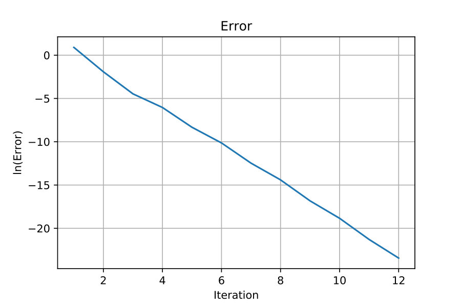 Figure 1
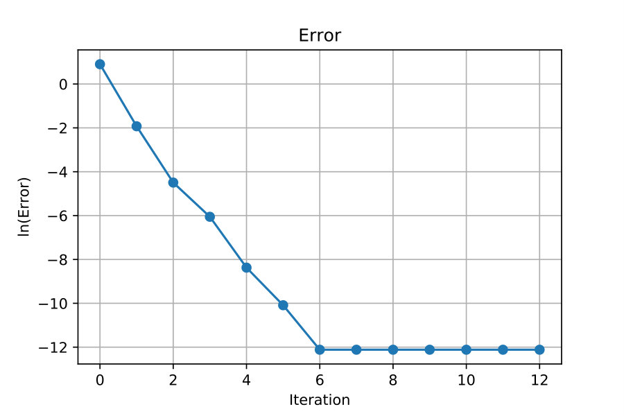 Figure 2
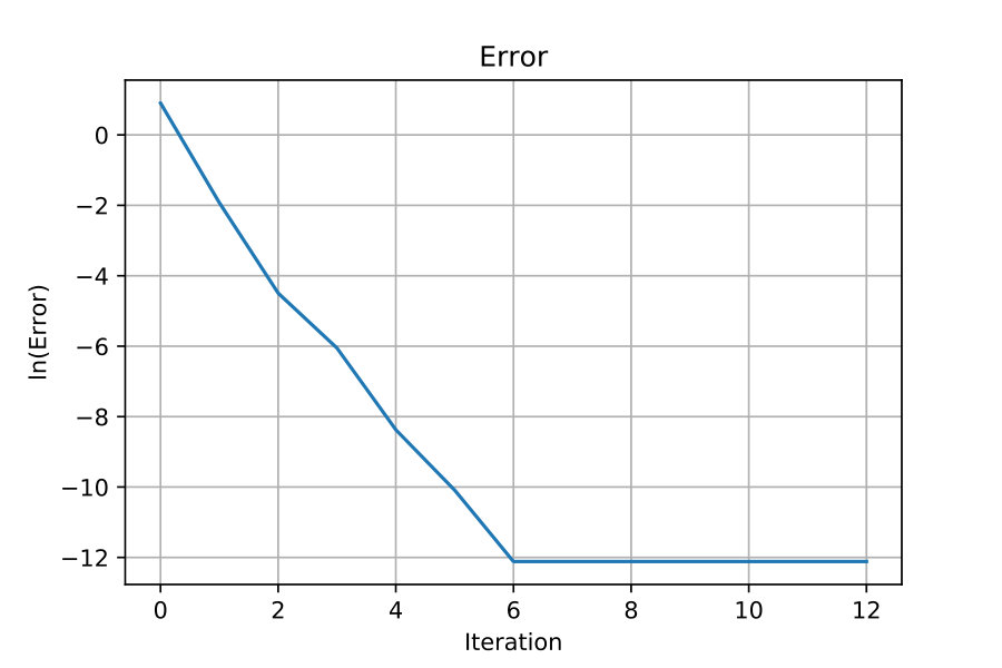 Figure 3
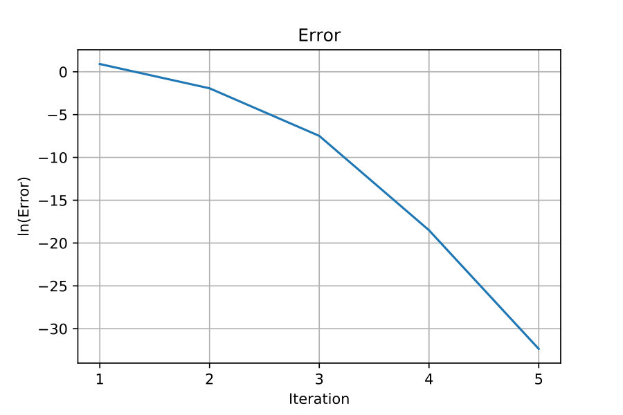 Figure 4
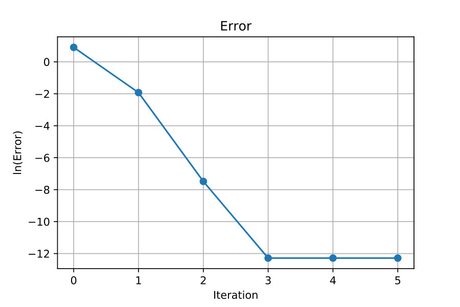 Figure 5
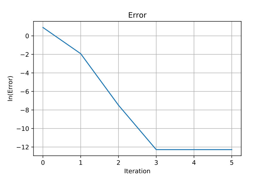 Figure 6
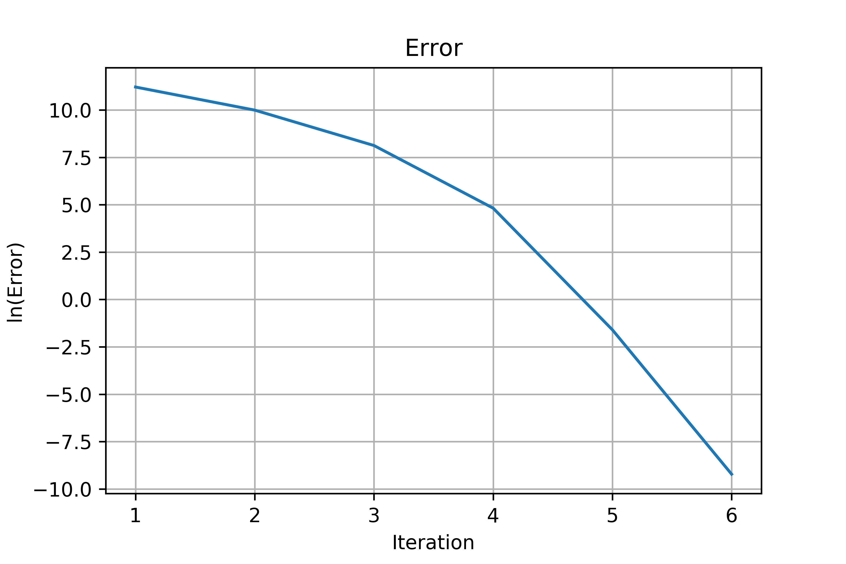 Figure 7
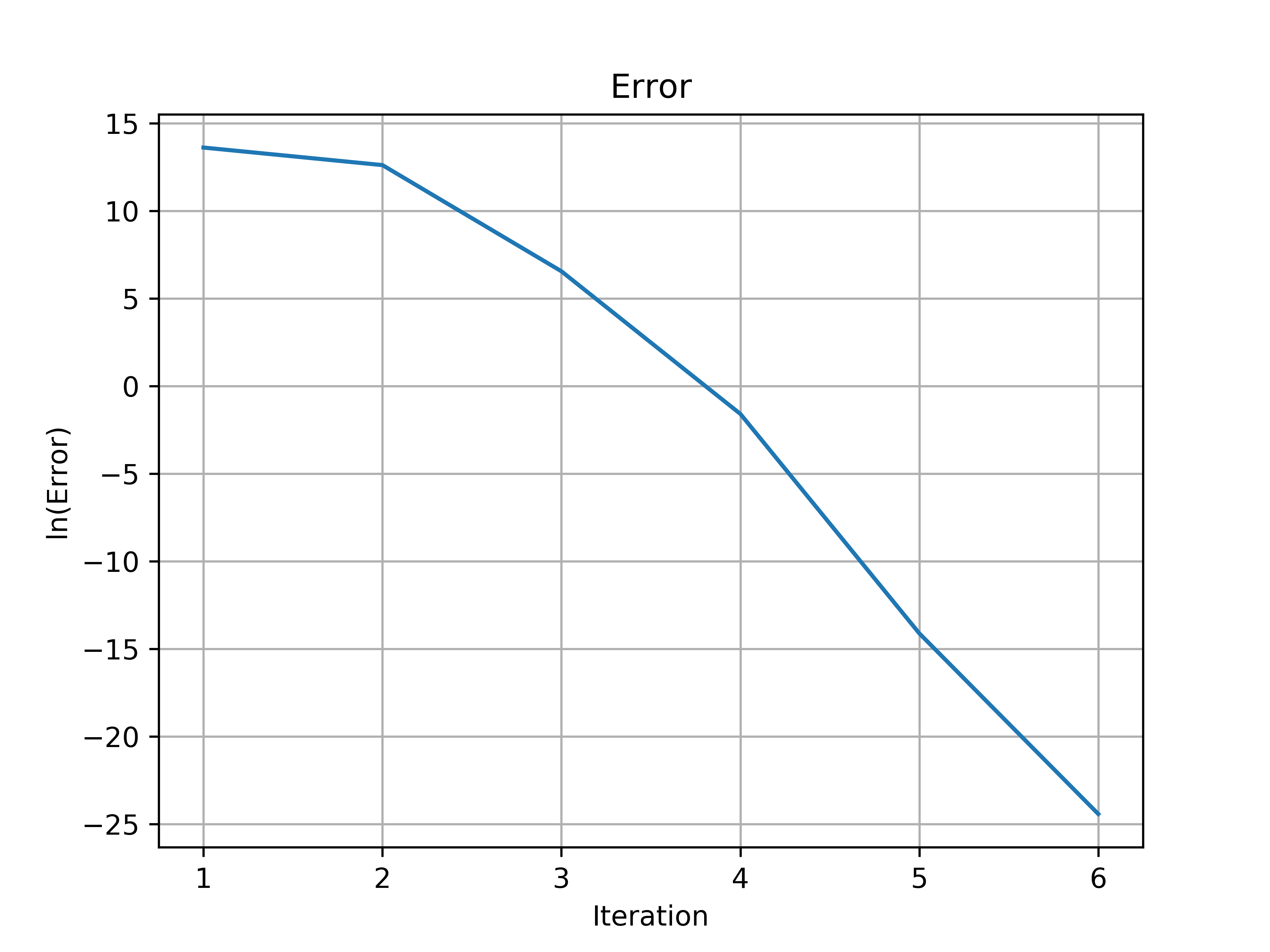 Figure 8
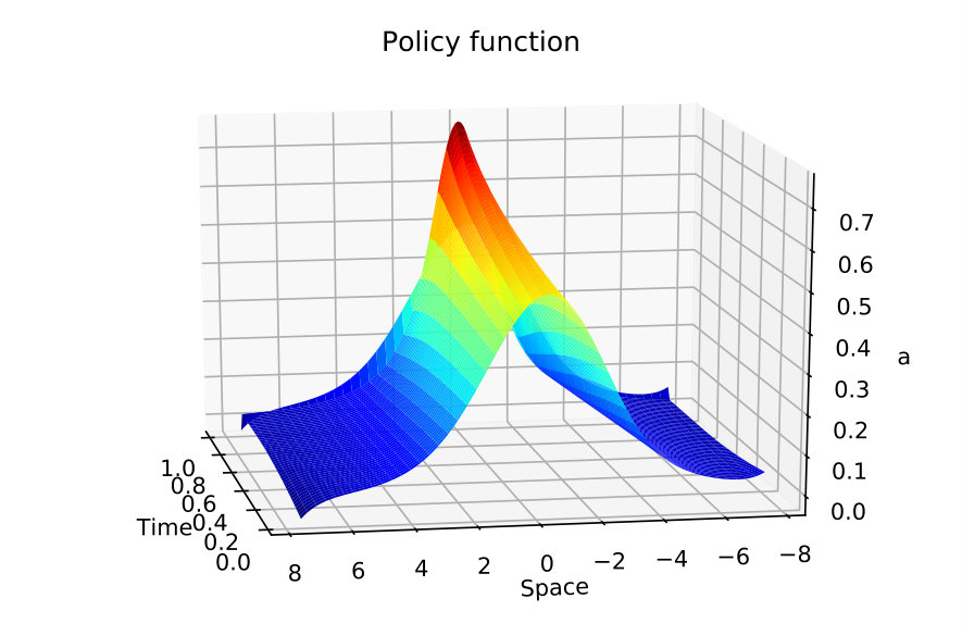 Figure 9
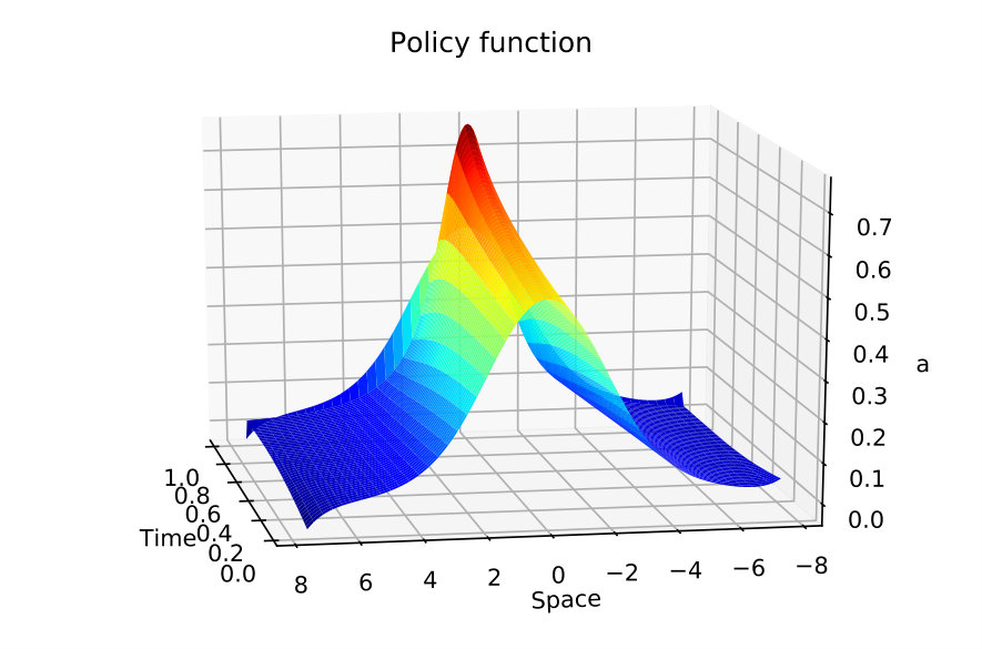 Figure 10
 Figure 11
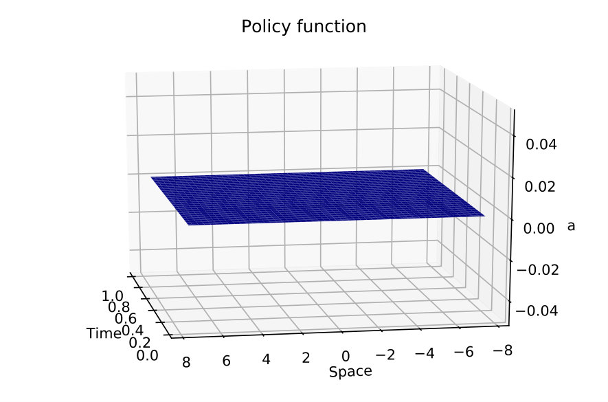 Figure 12
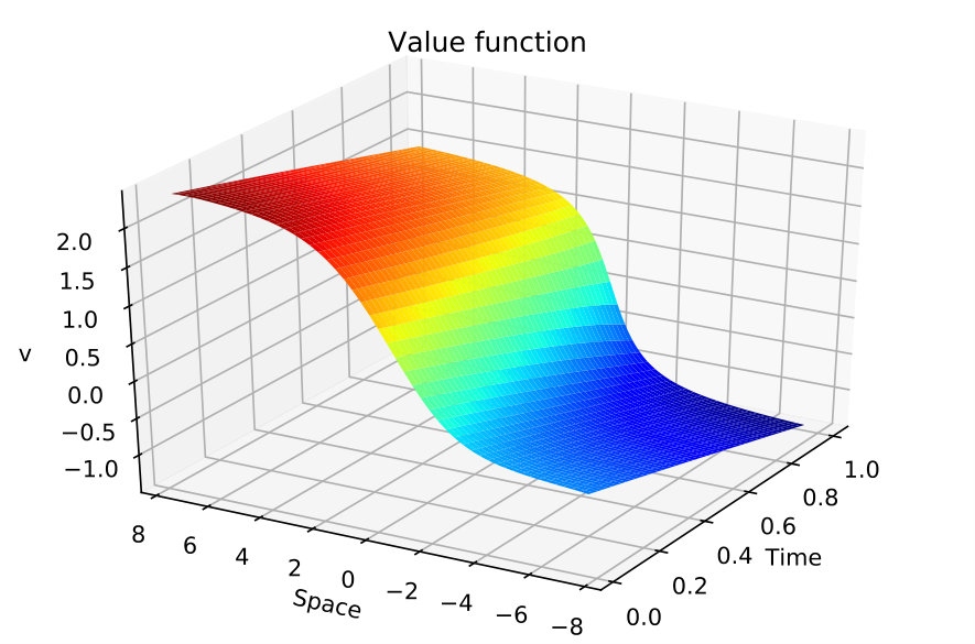 Figure 13
Peer Reviews
No public reviews on file for this paper yet. If you reviewed it on a platform where reviews are public (OpenReview, ICLR, NeurIPS, ICML), you can paste yours below so the community can read it here.
Videos
No videos yet. Explain this paper in a talk, walkthrough, or lecture? Add one.
Exponential Convergence and stability of Howard’s Policy Improvement Algorithm for Controlled Diffusions
B. Kerimkulov
Maxwell Institute Graduate School in Analysis and its Applications, Edinburgh, UK.
,
D. Šiška
School of Mathematics, University of Edinburgh and Vega Protocol
and
Ł. Szpruch
School of Mathematics, University of Edinburgh and Alan Turing Institute
(Date: 9th March 2024, )
Abstract.
Optimal control problems are inherently hard to solve as the optimization must be performed simultaneously with updating the underlying system. Starting from an initial guess, Howard’s policy improvement algorithm separates the step of updating the trajectory of the dynamical system from the optimization and iterations of this should converge to the optimal control. In the discrete space-time setting this is often the case and even rates of convergence are known. In the continuous space-time setting of controlled diffusion the algorithm consists of solving a linear PDE followed by a maximization problem. This has been shown to converge; in some situations, however no global rate is known. The first main contribution of this paper is to establish global rate of convergence for the policy improvement algorithm and a variant, called here the gradient iteration algorithm. The second main contribution is the proof of stability of the algorithms under perturbations to both the accuracy of the linear PDE solution and the accuracy of the maximization step. The proof technique is new in this context as it uses the theory of backward stochastic differential equations.
Key words and phrases:
Policy Improvement Algorithm, Stochastic Control, Backward Stochastic Differential Equation
2010 Mathematics Subject Classification:
93E20, 60H30, 65N12, 49L20
Supported by the Maxwell Institute Graduate School in Analysis and its Applications, a Centre for Doctoral Training funded by the UK Engineering and Physical Sciences Research Council (grant EP/L016508/01), the Scottish Funding Council, Heriot-Watt University and the University of Edinburgh.
1. Introduction
Stochastic control problems arise naturally in a range of applications in engineering, economics, and finance. Apart from very specific cases such as linear-quadratic control in engineering or the Merton portfolio optimization task in finance, stochastic control problems typically have no closed form solutions and have to be solved numerically. In this paper we consider the policy iteration algorithm and gradient iteration algorithm; see Algorithms 1 and 2. These are effectively a linearization method for the inherently nonlinear problem and play an essential role in numerical solutions of stochastic control problems.
We will consider the continuous space, continuous time problem where the controlled system is modeled by an -valued diffusion process. Let be a -dimensional Wiener martingale on a filtered probability space . Let us fix a finite time and consider the controlled SDE
[TABLE]
Here is a control belonging to the space of admissible controls , valued in , and we will write to denote the solution of (1) which starts from at time while being controlled by . We shall consider the gain functional in the form
[TABLE]
for all and . The value function is given for all and by
[TABLE]
We wish to solve the optimization problem, i.e., to find either the value function or the optimal control which achieves the maximum (or, if the supremum cannot be reached by , then an -optimal control such that ). It is well known that (see, e.g., Krylov [6]) that under reasonable assumptions the value function satisfies the Bellman PDE:
[TABLE]
Moreover (again see Krylov [6]), it is sufficient to consider Markovian controls, i.e., processes for some measurable function . Thus if we have obtained the value function, then we can find the optimal control (if it exists) as
[TABLE]
It is rarely possible to find a closed form solution to (4) and so various approximations have to be employed. One may, for example, choose to use a finite difference method to discretize (4) and indeed this has been widely studied; see, e.g., [12] or [14] and references therein. This results in a high dimensional nonlinear system of equations that still retains the structure of (4). To solve this nonlinear system one may apply the Howard’s policy improvement algorithm. The rate of convergence would then follow from results available on discrete space-time control problems. However, to check that the assumptions required for convergence are satisfied is not straightforward and moreover it is dependent on the discretization scheme used.
An alternative approach is to linearize (4) and to iterate. The classical approach is the Bellman–Howard policy improvement/iteration algorithm. The algorithm is initialized with a “guess” of the Markovian control. Given a Markovian control strategy at step one solves a linear PDE with the given control fixed and then one uses the solution to the linear PDE to update the Markovian control. In this paper we will show that this policy improvement algorithm (see Algorithm 1) and a variant which we call the gradient iteration algorithm (see Algorithm 2) converge, under appropriate assumptions, exponentially fast.
Iterative algorithms for the solution of optimal control problems go back to the work of Bellman [1, 2] where the value iteration algorithms for finite space-time problems are developed and their convergences are shown. Howard [3] proposed the policy improvement algorithm in the context of the discrete space-time Markovian decision rocess. Puterman and Brumelle’s paper [4] was one of the first results on the convergence properties for the policy iteration for MDP problems. The abstract function space setting employed in the paper applies to both discrete and continuous settings. Their main observation is that the policy iteration can be viewed as a type of Newton’s method. Hence similar convergence results to those known for Newton’s method follow: in particular, if the initial guess is in a neighborhood of the true solution, then the convergence will be quadratic. Puterman [5] applied this in a setting very similar to that of this paper to prove quadratic convergence in the neighborhood of the limit. Santos and Rust [9] consider the discrete time but continous space and controls setting. They extend the results of Puterman and Brumelle [4] to show global convergence, but without global rate, and quadratic local convergence rate of policy iteration and superlinear local convergence under more general conditions. In the case of stochastic control problems with jump-diffusion processes, Bäuerle and Rieder [17] have proved a convergence result of the Howard’s policy improvement algorithm with the help of martingale techniques. In the fully discrete space and time setting Bokanowski, Maroso, and Zidani [13] have shown global superlinear convergence, under a monotonicity assumption on the matrices defining the control problem. Convergence of policy iteration has been recently proved by Jacka and Mijatović [18] and Jacka, Mijatović, and Siraj [19]. Further, Maeda and Jacka [20] have shown quadratic local convergence of the policy iteration algorithm for the time-independent control problem. The local quadratic convergence is similar to the result of Puterman [5] but the specific control problem is different and moreover they employ a completely different technique based on Schauder estimates for linear PDEs.
The main contributions of this paper are to establish a global rate of convergence and stability for the policy iteration algorithm and a variant, which we call the gradient iteration algorithm. The analysis is carried out using backward stochastic differential equations (BSDEs) and to the best knowledge of the authors this is the first time BSDEs have been used to study convergence of the policy iteration algorithm. The assumptions required for this are effectively Lipschitz dependence in the drift, diffusion, instantaneous payoff, and terminal payoff functions and independence of the diffusion matrix on the control; see (1). The stability results show that the policy iteration remains stable even if the linear PDE is solved only approximately and even if the maximization is step performed approximately. Moreover they allow one to devise computationally efficient algorithms as they show that in the initial steps it is sufficient to solve the linear PDE with very low accuracy, and a highly accurate PDE solver is only required for the final few iterations of the algorithms.
The paper is organized as follows. In Section 2 we introduce all the assumptions and notation used throughout the paper. In Sections 3 and 4 we state and prove the results concerning convergence of the gradient iteration algorithm and the policy improvement algorithm, respectively. Section 5 justifies the name “policy improvement algorithm” in that it shows that the value functions increase monotonically with iterations and it also shows that the algorithm converges under weaker assumptions than those required for obtaining the rate. Sections 6 and 7 prove the stability of the algorithms. In Section 8 we present an example that fits the setting of this paper. Finally, in Appendix A, we collect several known results from the theory of BSDEs that are essential for the proofs.
We would like to emphasize that Algorithm 1 and Algorithm 2 are different, although they look rather similar. In Algorithm 1, is the value function for the Markov control , since it solves the PDE (5). In Algorithm 2 is not the value function for the Markov control . This is due to the term in the linear PDE (8).
2. Assumptions and Notation
We fix a finite horizon . We assume that for some we have such that . This is the space where the control processes take values. We fix a filtered probability space . Let be a -dimensional Wiener martingale on this space. Moreover, we have the following:
- (i)
For and a predictable process let us define
[TABLE]
For we will write . We will use to denote the set of all predictable processes such that . Note that the norm is equivalent to the norm for any . 2. (ii)
Let be the set of real valued -adapted continuous processes on such that
[TABLE] 3. (iii)
For adapted processes such that almost surely we will define
[TABLE] 4. (iv)
For any continuous local martingale let with denote the quadratic variation process and moreover let
[TABLE]
We are given measurable functions
[TABLE]
The state of the system is governed by the controlled SDE (1).
Assumption 2.1**.**
The functions and are continuous in . There exists and such that ,
[TABLE]
and
[TABLE]
Under Assumption 2.1 we know that for any and for any progressively measurable -valued control process there is a unique strong solution to (1) which we denote . Let
[TABLE]
be two given measurable functions. Let us assume the following for the running gain function and the terminal gain function appearing in (2).
Assumption 2.2**.**
There is a constant such that
[TABLE]
and
[TABLE]
Under Assumption 2.2 the gain functional given by (2) and the value function given by (3) are well defined. Moreover, the value function satisfies the Bellman equation (with derivatives existing almost everywhere, see Krylov [6, Chapter 4], or in the sense of viscosity solutions, see, e.g., Pham [15] or Fleming and Soner [11])
[TABLE]
Let us now state the additional assumptions required for our convergence result.
Assumption 2.3**.**
Let us define for each fixed the function
[TABLE]
We assume that the function is measurable.
If the function is convex for each fixed , which is in , one can immediately see that Assumption 2.3 holds. More generally, this assumption can be verified using an appropriate measurable selection theorem. For example, if is compact, then [7, Proposition D.5] shows that an appropriate measurable selection exists. If is not compact but is bounded, then [7, Proposition D.6] gives the same conclusion (using also that and Remark 2.8).
Assumption 2.4**.**
There are constants such that the following hold:
- (1)
(On the drift) For all , , ,
[TABLE]
and for all , , we have
[TABLE] 2. (2)
(On the control function) For all , , we have that
[TABLE]
[TABLE] 3. (3)
(On the running reward)
[TABLE]
Remark 2.5**.**
Under Assumptions 2.2 and 2.4 we have that for all , the following hold:
[TABLE]
and
[TABLE]
Under Assumptions 2.1, 2.2, 2.3, and 2.4 there is an optimal control process and this fact will be used to prove the main results.
Remark 2.6**.**
Due to results of Krylov [6] we know that (4) has a unique solution and moreover the map is bounded; see [6, Chapter 4, section 1, Theorem 1]. Hence, by Assumptions 2.3 and 2.4 we know that is jointly measurable and Lipschitz in . Thus, for each , the SDE
[TABLE]
has a unique solution . Then by the verification theorem, the process is the optimal control process for (3).
All the proofs will be completed in a new measure on given in the following lemma. We will use to denote the expectation under the measure .
Lemma 2.7**.**
Let Assumptions 2.1 and 2.2 together with (16) hold. Let . Let be the solution to the SDE (1) started from and controlled by the optimal control process . Then is a probability measure equivalent to and the process
[TABLE]
is a -Wiener process.
Proof.
This is an immediate consequence of (16) and Girsanov’s theorem. ∎
Remark 2.8**.**
From Krylov [6, Chapter 4, section 1, Theorem 1] we get that there is a constant such that for all we have that .
3. Convergence of gradient iteration algorithm
The following theorem gives the convergence result for Algorithm 2.
Theorem 3.1**.**
Let Assumptions 2.1, 2.2, 2.3, and 2.4 hold. Let be the solution to (4) and let be the approximation sequence given by Algorithm 2. Then there is depending only on and the initial guess such that for all there exists such that
[TABLE]
The main idea of the proof consists of noticing that Algorithm 2 can be seen as an iteration on the level of BSDEs. Using Lemma A.2 we see that on the level of BSDEs this iteration is contractive. Finally we need to use known results on the connection between BSDEs and solutions to the HJB equation.
Proof of Theorem 3.1.
We prove the main result in several steps. First, we show how to rewrite the gradient iteration algorithm as an iteration on the level of BSDEs. On the th step of the algorithm we need to solve the linear PDE with Lipschitz continuous coefficients (8). Let be the solution to (8) and recall that
[TABLE]
Since we are working with the linear PDE with Lipschitz continuous coefficients, we have in . Let be the solution to the SDE (1) started from and controlled by the optimal control process ; see Remark 2.6. From Itô’s formula we then get that
[TABLE]
Let
[TABLE]
and
[TABLE]
Then we may write
[TABLE]
Let and be given by Lemma 2.7. Hence (18) becomes
[TABLE]
Consider now the following BSDE:
[TABLE]
where the superscript means that the forward process started from . Hence, we can define
[TABLE]
Therefore by (14) we have
[TABLE]
Thus, by Pham [15, Theorem 6.3.3], the function solves the HJB equation (4). Notice that here is the crucial point where the fact that we use the optimal control plays a role. Indeed with other control processes we couldn’t claim that solves the HJB equation. By uniqueness of the viscosity solution to the HJB equation (see the strong comparison principle from [15, Theorem 4.4.5]), we can conclude that and therefore is the value function of our stochastic control problem. Therefore, the BSDE (20) is the BSDE corresponding to the value function. Notice that (20) is a quadratic BSDE, since in the generator we have a product of two Lipschitz functions which depend on . The existence of the solution to (20) under our assumptions can be obtained by applying Theorem A.9 in the case when the terminal cost is bounded for our stochastic control problem.
Using Remark 2.8, the fact that , and Assumption 2.4, for all we get that
[TABLE]
Moreover, recalling , we get that from the higher moment estimates for the solution of the SDE and from the Lipschitz property of . Similarly by Assumption 2.4. We may thus apply Lemma A.2 and hence, due to (19) and (22), we have and such that for all
[TABLE]
Therefore, from (21) and (17), we have and and by (23) we obtain
[TABLE]
Hence
[TABLE]
This finishes the proof. ∎
4. Convergence of policy improvement
Theorem 4.1**.**
Let Assumptions 2.1, 2.2, 2.3, and 2.4 hold. Let be the solution to (4) and let be the approximation sequence given by Algorithm 1. Then there is depending only on and the initial guess such that for all there exists such that
[TABLE]
The proof of Theorem 4.1 is similar to that of Theorem 3.1 except that the iteration on the level of BSDEs is nonstandard.
Proof of Theorem 4.1.
Let be the solution to (5) and recall that
[TABLE]
As before, let be the solution to the SDE (1) started from and controlled by the optimal control process ; see Remark 2.6. By Itô’s formula
[TABLE]
Let
[TABLE]
Recalling that the control and the associated diffusion are fixed we can write
[TABLE]
Let and be given by Lemma 2.7. Then (24) becomes
[TABLE]
Similarly as in Theorem 3.1, consider the BSDE
[TABLE]
In same way we can show that is the value function of our stochastic control problem. As before, from Krylov [6, Chapter 4, section 1, Theorem 1], we get that there is a constant such that for all we have that . Moreover, as before, using Remark 2.8, the fact that , and Assumption 2.4, for all we get that
[TABLE]
Finally we note that and , so by Lemma A.5, together with (25) and (26), we have and such that for all
[TABLE]
Similarly as before, using (28), we conclude that
[TABLE]
This concludes the proof of the theorem. ∎
Remark 4.2**.**
Consider briefly the situation where the diffusion coefficient also depends on the control, i.e., . After applying Itô’s formula to and substituting the solution to the linear PDE for we get
[TABLE]
*The resulting object can be seen as a second order BSDE (2BSDE). Analysis of 2BSDEs goes beyond the scope of this paper. *
Remark 4.3**.**
Let us briefly consider the infinite-time-horizon control problem. In this case we consider a constant and the gain functional:
[TABLE]
It is known that the Bellman PDE for the value function is
[TABLE]
The linear PDE from the iteration of the policy improvement algorithm then is
[TABLE]
where
[TABLE]
After applying Itô’s formula we get
[TABLE]
Let and . Then after change of measure we may write
[TABLE]
Let
[TABLE]
Hence (29) becomes
[TABLE]
To proceed, we need a suitable contraction-type inequality for this infinite time horizon BSDE. Buckdahn and Peng [8] studied infinite time horizon BSDEs and have proved existence and uniqueness of their solutions for sufficiently large values of . To get the required contraction-type inequality we can use similar calculations as in Fuhrman and Tessitore [10, Theorems 3.2 and 3.7], where they use Banach’s fixed point theorem to show existence and uniqueness of solutions to infinite time horizon BSDEs. Hence, for sufficiently large we would obtain results analogous to Theorem 4.1 as well as the other theorems in the article.
5. Policy improvement
We want to show that the policy obtained at each step of Algorithm 1 is an improvement on the one from the previous step. This is formulated as Theorem 5.1 below. Note that we do not require Assumption 2.4 here.
Theorem 5.1**.**
Let Assumptions 2.1, 2.2, and 2.3 hold. Assume that there exists such that , , and
[TABLE]
Fix . Let and be the solutions of (5) at steps and of the algorithm. Then for all , it holds that
[TABLE]
Proof.
Let be the solution to the SDE (1) started from and controlled by the optimal control process ; see Remark 2.6. Then, as in the proof of Theorem 4.1, we get that for with and with we have the BSDE representation
[TABLE]
where
[TABLE]
Let us denote for and
[TABLE]
Hence, notice that by the definition of the (see (6)), we have for all that
[TABLE]
Therefore by the comparison principle for BSDEs (see Lemma A.6), we get
[TABLE]
Hence, we have
[TABLE]
∎
Remark 5.2**.**
It is perhaps interesting to note that the comparison principle for BSDEs cannot be used to deduce that in the gradient iteration algorithm we have an “improvement” at each step. Indeed, let us write the BSDE representation of the two steps of gradient iteration for ,
[TABLE]
and
[TABLE]
where
[TABLE]
In order to apply a comparison principle for BSDEs (see Lemma A.6), we would need to have . Nevertheless we observe that
[TABLE]
Similarly,
[TABLE]
From the above calculations we have no way to conclude that . Thus the gradient iteration algorithm is not guaranteed to be improving the policy with each step.
6. Stability under Perturbations to Solution of the Linear PDE
In this section we study a stability property of the policy improvement algorithm under perturbations to solutions of the linear PDE (5) since in practical applications one will only solve this equation approximately. Of course the maximization step (6) of Algorithm 1 can now be performed only with this approximate solution, thus feeding the errors into further iterations.
Let be a parameter (or a set of parameters), which determines the accuracy of our approximation to the solution of the linear PDE (5). Let be the policy at iteration obtained from an approximate solution to the linear PDE. Let denote the solution to
[TABLE]
At step of Algorithm 1 we approximate the solution to the equation above (this is PDE (5) but with replacing everywhere). We will denote such approximation by . The policy function for the next iteration step is then given by
[TABLE]
recalling that the function was defined in (14). We need to assume that is bounded so that is Lipschitz in so that the solution to (31) is . This assumption is not really a restriction as we know that the gradient of the value function is bounded under our assumptions; see Krylov [6, Chapter 4, section 1, Theorem 1] and also Remark 2.6. Any reasonable approximation should retain this property.
Theorem 6.1**.**
Let Assumptions 2.1, 2.2, 2.3, and 2.4 hold. Let be the approximation sequence given by Algorithm 1. Let be the approximation sequence given by (31). Let and be the optimal control process for (3) and the associated diffusion started from . Assume that is uniformly bounded. Define
[TABLE]
Then there is and , depending only on , such that for all there exists such that
[TABLE]
Proof.
Let be the solution to the SDE (1) started from and controlled by the optimal control process ; see Remark 2.6. By applying Itô’s formula to we get
[TABLE]
Let us denote
[TABLE]
[TABLE]
and
[TABLE]
where is an approximate solution to corresponding PDE. Then using this notation, we may write
[TABLE]
Let and be given by Lemma 2.7. Then the above equation becomes
[TABLE]
We want to study the difference of with , where solves the BSDE (25).
[TABLE]
where solves the BSDE (26). Due to (27) and
[TABLE]
we can apply Lemma A.5. Hence, there is and such that
[TABLE]
and
[TABLE]
Therefore we continue the estimate (32)
[TABLE]
This concludes the proof of the theorem. ∎
7. Stability under Perturbation of the Maximization
In this section we study a stability property of the gradient iteration algorithm under perturbations to maximization procedure (7). Let be the solution to corresponding PDE at iteration of the gradient iteration algorithm, where instead of obtaining the control function corresponding to the exact maximum
[TABLE]
we only solve this maximization problem approximately and so we are dealing with a control function of the form
[TABLE]
where the function determines the accuracy of our approximation.
Theorem 7.1**.**
Let Assumptions 2.1, 2.2, 2.3, and 2.4 hold. Let be the approximation sequence given by Algorithm 2. Let be the approximation sequence given by the perturbations to the maximization procedure and assume that . Let and be the optimal control process for (3) and the associated diffusion started from . Define
[TABLE]
[TABLE]
Then there is and , depending only on , such that for all there exists such that
[TABLE]
Proof.
Let be the solution to the SDE (1) started from and controlled by the optimal control process ; see Remark 2.6. As in the proof of Theorem 3.1 we can write two BSDEs we get after the change of measure given by Lemma 2.7. The first BSDE arises from the perturbations of the maximization:
[TABLE]
where
[TABLE]
The second BSDE arises from the gradient iteration algorithm with the maximization performed exactly:
[TABLE]
where
[TABLE]
We want to study the difference of with . Hence, notice that
[TABLE]
where solves (20). Therefore, since
[TABLE]
we can apply Lemma A.7 so that there is and such that
[TABLE]
Now we need to estimate the second term of the right-hand side (RHS). Notice that by Assumption 2.4 the following holds:
[TABLE]
Hence by (35) we have
[TABLE]
By inequalities (33), (34), (36), and the result of Theorem 3.1 and since as well as , we conclude that
[TABLE]
∎
We obtain the same result for the policy improvement algorithm.
Theorem 7.2**.**
Let Assumptions 2.1, 2.2, 2.3, and 2.4 hold. Let be the approximation sequence given by Algorithm 1. Let be the approximation sequence given by the perturbations to the maximization procedure. Let and be the optimal control process for (3) and the associated diffusion started from . Define
[TABLE]
[TABLE]
Then there is and , depending only on , such that for all there is such that
[TABLE]
Proof.
Let be the solution to the SDE (1) started from and controlled by the optimal control process ; see Remark 2.6. Due to Theorem 4.1 we can write two BSDEs we get after the change of measure: first from the perturbation and second from the gradient iteration
[TABLE]
[TABLE]
where
[TABLE]
[TABLE]
Similarly, we want to study the difference of with . Hence, notice that
[TABLE]
where solves (4.1). Therefore, since
[TABLE]
we can apply Lemma A.8 so that there is and such that
[TABLE]
Now we need to estimate the second term of the RHS. Notice that by Assumption 2.4 we have that
[TABLE]
Hence by (39) we have
[TABLE]
By inequalities (37), (38), (40), by the result of Theorem 4.1, and by , we conclude that
[TABLE]
∎
8. Example
In this section we would like to consider an example when Assumptions 2.1, 2.2, 2.3, and 2.4 hold. Let and be continuous functions for . Consider the state which is governed by the controlled SDE
[TABLE]
and consider the cost functional
[TABLE]
The aim is to maximize over admissible controls . The value function satisfies the Bellman PDE
[TABLE]
with the terminal condition . Hence, the optimal control is
[TABLE]
It is easy to check that Assumptions 2.1, 2.2, 2.3, and 2.4 hold for this problem. Therefore, the Bellman PDE becomes
[TABLE]
We can solve this problem using the policy improvement algorithm by approximating the Bellman PDE with a sequence of linear PDEs:
Step 1. Make an initial choice of control .
Step 2. For :
- •
Evaluation step: Find a solution to the linear PDE
[TABLE]
- •
Improvement step: Find a new policy such that
[TABLE]
Step 3. Iterate the process until no changes occur in the controls updates.
One can do similar calculations in the case of the gradient iteration algorithm.
We will solve (41) and (42) by the finite difference method. For simplicity, let us choose and for all . In Figure 8.1, one can see the logarithm of the error between the value function obtained by the iterative methods, by the policy improvement algorithm, and by the gradient iteration algorithm at every step and the value function obtained by the solution of the Bellman PDE. This shows the fast convergence of the policy improvement method for our example in one dimension. In Figure 8.2, we can see that after only a few steps the policies obtained from the policy improvement algorithm are close to the exact one. Finally, in Figure 8.3, we plot the value function and the policy from the solution of the Bellman PDE.
Appendix A Some results from theory of BSDEs
We fix a finite horizon . We fix a filtered probability space . Let there be a -dimensional Wiener martingale on this space.
Lemma A.1**.**
Let be a measurable function that satisfies the following conditions: The process is in . Moreover there is a constant such that
[TABLE]
Then, for every and , there is a unique solution to
[TABLE]
Proof.
This follows immediately from, e.g., Pham [15, Theorem 6.2.1]. ∎
Lemma A.2**.**
Let satisfy the hypothesis of Lemma A.1. Fix . Let , where is the unique solution to (43). Moreover assume that for the following condition satisfies that there is a constant such that
[TABLE]
Then there is and such that for , , and any we have
[TABLE]
The proof is well known and is included, e.g., as part of Pham [15, Proof of Theorem 6.2.1]. We provide it here for the convenience of the reader and before we proceed we need to make the following observation.
Remark A.3**.**
Assume that and and let
[TABLE]
Then and hence is a uniformly integrable martingale. Indeed, from the Burkholder–Davis–Gundy inequality and the Young inequality we get
[TABLE]
Proof of Lemma A.2.
Consider which we will fix later. We denote , , , and . We then apply Itô’s formula to :
[TABLE]
Due to Remark A.3, the stochastic integral vanishes by taking expectation. Hence
[TABLE]
By the Lipschitz property of the generator and by the Young inequality we continue our estimate, noting that for any , we have
[TABLE]
Choose such that . Thus
[TABLE]
Hence, from (45) we have that for and any
[TABLE]
where . This concludes the proof of the lemma. ∎
Lemma A.4**.**
Let be a measurable function such that the process is in and such that there are so that for all , we have
[TABLE]
If and , then there is a unique solution to
[TABLE]
Proof.
This follows immediately from, e.g., Pham [15, Theorem 6.2.1]. ∎
Lemma A.5**.**
Let satisfy the hypothesis of Lemma A.4. Fix . Let , where is the unique solution to (46). Moreover assume that for the following condition satisfies that there are constants such that
[TABLE]
where , . Then there is and such that for any we have
[TABLE]
Moreover, there is such that .
Proof.
Consider which we will fix later. We denote , , and . We then apply Itô’s formula to :
[TABLE]
The expectation of the stochastic integral is [math] due to Remark A.3. Hence, by taking expectation we derive from the equality above that
[TABLE]
By the Lipschitz property of the generator and by the Young inequality we observe that, for any ,
[TABLE]
Take sufficiently large so that . Choose such that . Thus
[TABLE]
Dividing by we obtain
[TABLE]
where . Since we have that . Therefore from (47) we have for any
[TABLE]
By choosing such that we get that . This concludes the proof of the lemma. ∎
We now state a comparison principle for BSDEs.
Lemma A.6**.**
Consider the following BSDEs:
[TABLE]
Assume that , , and a.s. Let , , be such that for all the processes are progressively measurable, , and such that there is so that for all , we have
[TABLE]
Moreover, suppose that for it holds that
[TABLE]
Then for all a.s.
Proof.
This follows from, e.g., Pham [15, Theorem 6.2.2]. ∎
The following two lemmas are auxiliary results we need in Section 7.
Lemma A.7**.**
Let be measurable functions and let satisfy the hypotheses of Lemmas A.1 and A.2. Fix . Let and be such that
[TABLE]
and
[TABLE]
Then there is and such that for we have
[TABLE]
Proof.
Consider which we will fix later. We denote , , and . We then apply Itô’s formula to :
[TABLE]
Due to Remark A.3, the stochastic integral vanishes by taking expectation. Hence
[TABLE]
Notice that due to (44) for all it holds that
[TABLE]
Then by the Young inequality we continue our estimate (48), noting that for any , we have
[TABLE]
Fix and . Let . Then
[TABLE]
This concludes the proof of the lemma. ∎
Lemma A.8**.**
Let be a measurable function and let satisfies the hypotheses of Lemmas A.4 and A.5. Fix . Let and be such that
[TABLE]
and
[TABLE]
Then there is and such that for we have
[TABLE]
Proof.
Consider which we will fix later. We denote , , and . We then apply Itô’s formula to :
[TABLE]
Due to Remark A.3, the stochastic integral vanishes by taking expectation. Hence
[TABLE]
Notice that by assumptions of the lemma for all it holds that
[TABLE]
Then by the Young inequality for any , we have
[TABLE]
Let us take sufficiently large so that . Let so that
[TABLE]
Dividing by we obtain
[TABLE]
where . Since we have that . ∎
A.1. BSDE with drivers of quadratic growth.
Since we are using BSDE theory in the proof of the main result, we would like to present some results on BSDE with drivers of quadratic growth. We refer to [16].
Consider the following system:
[TABLE]
Theorem A.9** (Theorem 3.6 in [16]).**
Let and be Lipschitz continuous with Lipschitz constant and and for all . Let and be measurable functions and let us assume that there exists constant such that for all , and
[TABLE]
There exists a solution of the Markovian BSDE (49) in and this solution is unique among solutions such that is bounded. Moreover, we have
[TABLE]
and
[TABLE]
where
[TABLE]
here the supremum is taken over all stopping times in .
The reference list from the paper itself. Each links out to its DOI / PubMed record.
- 1[1] R. Bellman, Functional equations in the theory of dynamic programming. V. Positivity and quasi-linearity, Proc. Natl. Acad. Sci. USA. , 41 (1955), pp. 743-746.
- 2[2] R. Bellman, Dynamic Programming , Princeton University Press, Princeton, NJ, USA, 1957.
- 3[3] R. A. Howard, Dynamic Programming and Markov Processes , MIT Press, Cambridge, MA, 1960.
- 4[4] M.L. Puterman and S. L. Brumelle, On the convergence of policy iteration in stationary dynamic programming, Math. Oper. Res. , 4 (1979), pp. 60-69.
- 5[5] M. L. Puterman, On the convergence of policy iteration for controlled diffusions, J. Optim. Theory Appl. , 33 (1981), pp. 137–144 .
- 6[6] N. V. Krylov, Controlled Diffusion Processes , Springer, New York, 1980.
- 7[7] O. Hernandez-Lerma and J. Lasserre, Discrete-Time Markov Control Processes , Springer, New York, 1996.
- 8[8] R. Buckdahn and S. Peng, Ergodic Backward SDE and Associated PDE, R.C. Dalang, M. Dozzi and F. Russo eds., Progr. Probab. 45 , Birkhäuser, Basel, 1999.