Exact Top Yukawa corrections to Higgs boson decay into bottom quarks
Amedeo Primo, Gianmarco Sasso, Gabor Somogyi, Francesco Tramontano

TL;DR
This paper provides an exact calculation of top Yukawa coupling contributions to Higgs decay into bottom quarks, confirming the accuracy of previous approximations and showing minimal impact on collider search distributions.
Contribution
It presents the first exact computation of top Yukawa corrections to Higgs to bottom quark decay, validating approximate methods and assessing their phenomenological significance.
Findings
Approximate results are highly accurate for physical masses.
Corrections have a small effect on differential distributions.
Results support the reliability of previous approximations.
Abstract
In this letter we present the results of the exact computation of contributions to the Higgs boson decay into bottom quarks that are proportional to the top Yukawa coupling. Our computation demonstrates that approximate results already available in the literature turn out to be particularly accurate for the three physical mass values of the Higgs boson, the bottom and top quarks. Furthermore, contrary to expectations, the impact of these corrections on differential distributions relevant for the searches of the Higgs boson decaying into bottom quarks at the Large Hadron Collider is rather small.
Click any figure to enlarge with its caption.
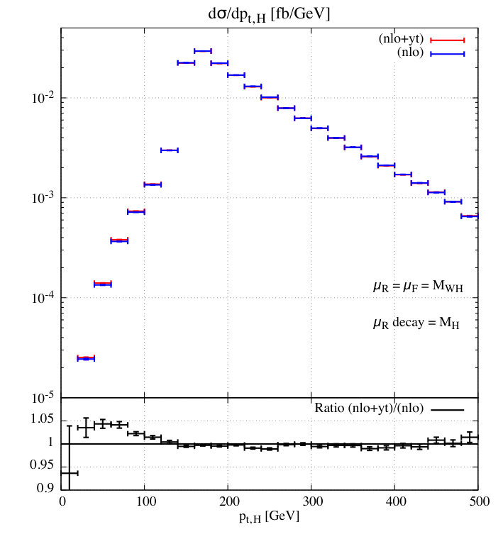 Figure 1
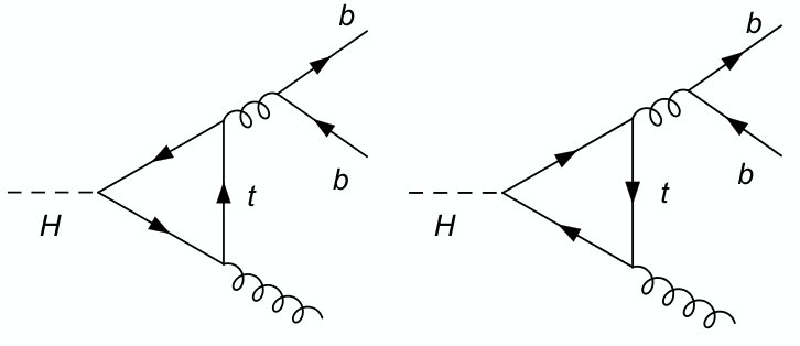 Figure 1
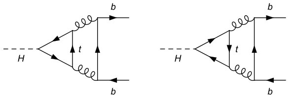 Figure 2
| 20 | 75 | 125 | 180 | |
|---|---|---|---|---|
| 100 | 2.123 | 0.075 | 1.025 | 6.704 |
| 125 | 2.329 | 0.011 | 0.335 | 2.107 |
| 175 | 2.452 | -0.019 | 0.018 | 0.355 |
| 250 | 2.566 | -0.024 | -0.055 | -0.035 |
| 350 | 2.656 | -0.023 | -0.069 | -0.113 |
Peer Reviews
No public reviews on file for this paper yet. If you reviewed it on a platform where reviews are public (OpenReview, ICLR, NeurIPS, ICML), you can paste yours below so the community can read it here.
Videos
No videos yet. Explain this paper in a talk, walkthrough, or lecture? Add one.
Exact Top Yukawa corrections to Higgs boson decay into bottom quarks
Amedeo Primo
Department of Physics, University of Zürich, CH-8057 Zürich, Switzerland
Gianmarco Sasso
Università di Napoli Federico II,
Complesso di Monte Sant’Angelo, Edificio 6
via Cintia I-80126, Napoli, Italy
Gábor Somogyi
MTA-DE Particle Physics Research Group, H-4010 Debrecen, PO Box 105, Hungary
Francesco Tramontano
Università di Napoli Federico II and INFN sezione di Napoli,
Complesso di Monte Sant’Angelo, Edificio 6
via Cintia I-80126, Napoli, Italy
Abstract
In this letter we present the results of the exact computation of contributions to the Higgs boson decay into bottom quarks that are proportional to the top Yukawa coupling. Our computation demonstrates that approximate results already available in the literature turn out to be particularly accurate for the three physical mass values of the Higgs boson, the bottom and top quarks. Furthermore, contrary to expectations, the impact of these corrections on differential distributions relevant for the searches of the Higgs boson decaying into bottom quarks at the Large Hadron Collider is rather small.
pacs:
††preprint: ZU-TH 48/18
I Introduction
The discovery of the Higgs boson Higgs (1964); Englert and Brout (1964) by the ATLAS Aad et al. (2012) and CMS Chatrchyan et al. (2012) experiments at CERN has ushered in a new era in particle physics phenomenology. The Standard Model (SM) of elementary particles is now complete and there is no decay or scattering phenomenon at low energies that significantly deviates from what is predicted by the SM. Still, we know that the SM cannot be the ultimate theory, if not for the lack of consistency with mainly cosmological observations, but for the fact that it contains quite a large number of parameters, which makes it unreasonable to think of it as a fundamental theory. The LHC is guiding the experimental community towards the study of the Higgs potential and the Higgs boson direct couplings with all the other particles, an experimentally previously completely unexplored sector of the SM Lagrangian. The SM makes very precise predictions for all the vertices and couplings of the Higgs boson and the verification of these predictions is among the fundamental questions addressed at the LHC.
In particular, the gluon fusion production mechanism has given direct access to Higgs boson decay into vector bosons and an indirect access the top Yukawa coupling. More recently, also the direct coupling of the Higgs boson to the top quark has been observed Aaboud et al. (2018a); Sirunyan et al. (2018a). Measurements of the Higgs coupling to the tau lepton have been extracted by combining all production modes Sirunyan et al. (2018b); Aaboud et al. (2018b), while the direct coupling to the bottom quark has been observed by exploiting the features of the VH (V = W or Z) associated production mechanism Aaboud et al. (2018c); Sirunyan et al. (2018c). The decay to bottom quarks is quite special, because it is the one with the largest branching ratio. The decay width of the Higgs boson into bottom quarks has been computed at up to four loops in QCD Gorishnii et al. (1990, 1991); Kataev and Kim (1994); Surguladze (1994); Larin et al. (1995); Chetyrkin and Kwiatkowski (1996); Chetyrkin (1997); Baikov et al. (2006) using an approximated treatment of the bottom quark mass, up to one loop including electroweak corrections Dabelstein and Hollik (1992); Kniehl (1992) and also including mixed QCD-electroweak effects Mihaila et al. (2015). The exact bottom mass corrections have been computed up to two loops Bernreuther et al. (2018). A relatively large component of the two loop computation is represented by the diagrams in which the Higgs boson couples to a top quark loop, see Figs. 1 and 2. These two sets of diagrams are both UV and IR finite separately, and their contributions have been computed only approximately in Chetyrkin and Kwiatkowski (1996), finding a very compact formula that should be considered valid for values of the masses such that . Comparing this formula with the rest of the two loop contributions, it turns out that these pieces, proportional to the top Yukawa coupling , account for about of the total two loop result.
The aim of this letter is twofold. First, we want to assess the impact of the neglected terms in the expansion of Chetyrkin and Kwiatkowski (1996), that in principle could be of the order of (see Eq. (3) in Chetyrkin and Kwiatkowski (1996)). We do this by computing the full analytic result for the contributions to the Higgs boson decay into bottom quarks that are proportional to the top Yukawa coupling, including the exact dependence on the top and bottom quark masses. Furthermore, recently two groups have computed the fully differential decay width of the Higgs boson into bottom quarks up to two loops for the massless case, and merged this computation to the two loop corrections to the associated production in hadronic collisions Ferrera et al. (2018); Caola et al. (2018). The corrections to key distributions like the transverse momentum and the mass spectra of the Higgs boson (reconstructed using the two hardest b-jets in the final state) are found to be very large. contributions to the Higgs decay into bottom quarks are not included in the differential results mentioned above and so it is natual to ask what the impact of these corrections is (see for example Caola et al. (2018)). We answer this second question by presenting differential results which include the contributions to the decay and retain the full mass dependence on the top and bottom quark masses.
II Calculation
II.1 Double virtual
The decay receives contributions from the interference of the Born amplitude with two loop virtual corrections that involve a closed top quark loop,
[TABLE]
where is given by the two diagrams shown in Fig. 1. By evaluating the Feynman diagrams, we decomposed as
[TABLE]
with and . In Eq. (2), the are rational coefficients and are two loop integrals of the type
[TABLE]
defined by the set of inverse propagators:
[TABLE]
with kinematics , .
We computed the loop integrals through the consolidated differential equations (DEs) method Kotikov (1991); Remiddi (1997); Gehrmann and Remiddi (2000); Argeri and Mastrolia (2007). First, we used integration-by-parts identities (IBPs) Tkachov (1981); Chetyrkin and Tkachov (1981); Laporta (2000), generated with the help of Reduze2 von Manteuffel and Studerus (2012), in order to reduce the integrals that appear in to a set of 20 independent master integrals (MIs) . Subsequently, we derived the analytic expression of the MIs by solving the system of coupled first-order DEs in the kinematic ratios and . The structure of the DEs, and hence of their solutions, is simplified by parametrizing such ratios in terms of the variables and , defined by
[TABLE]
and by using the Magnus exponential method Argeri et al. (2014); Di Vita et al. (2014); Bonciani et al. (2016); Di Vita et al. (2017); Mastrolia et al. (2017); Di Vita et al. (2018) in order to identify a basis of MIs that fulfil a system of canonical DEs Henn (2013),
[TABLE]
In Eq. (6), the coefficient matrix is a -form that contains 12 distinct letters,
[TABLE]
with . Since all letters are algebraically-rooted polynomials, we could derive the -expansion of the general solution of Eq. (6) in terms of two-dimensional generalized polylogarithms (GPLs) Goncharov (1995); Remiddi and Vermaseren (2000); Gehrmann and Remiddi (2001, 2002); Vollinga and Weinzierl (2005), by iterative integration of the -form, which we performed up , i.e. to GPLs of weight four. In order to fully specify the analytic expression of the MIs, we complemented the general solution of DEs with a suitable set of boundary conditions. The latter were obtained by demanding the regularity of the MIs at the pseudo-thresholds and that appear as unphysical singularities of the DEs.
The expression of the MIs obtained in this way is valid in the Euclidean region , where the logarithms of Eq. (7) have no branch-cuts and, hence, the MIs are real. The values of the MIs for positive values of the Higgs squared momentum, and in particular for the decay region , are obtained through analytic continuation, by propagating the Feynman prescription to the kinematic variables and . All results have been numerically validated with GiNaC Bauer et al. (2000) against the results of SecDec3 Borowka et al. (2015), both in the Euclidean and in the physical regions.
Upon inserting the expressions of the MIs into Eq. (2), we observed the expected analytic cancellation of all -poles and obtained a finite result for ,
[TABLE]
with being a polynomial combination, with algebraic coefficients, of 256 distinct GPLs. The explicit expression of , as well as of the newly computed MIs, can be released by the authors upon request.
II.2 Real-virtual
The real-virtual part of the computation involves the interference of the tree level amplitude for with the loop diagrams in Fig. 2 containing a closed top quark loop,
[TABLE]
We used standard techniques to evaluate the one loop amplitude. As expected, is finite (in ) and can be written as
[TABLE]
plus terms that vanish in four dimensions. In Eq. (10), denotes twice the dot-product of momenta, .
We integrated the real-virtual contribution over the whole phase space both analytically and numerically using Monte Carlo integration, finding perfect agreement. The analytic computation was performed by direct integration of over the three-particle phase space. The phase space measure for the decay reads
[TABLE]
where is given by
[TABLE]
The integral is finite in four dimensions and was evaluated in terms of GPLs after suitable transformations of the integration variables. In particular, square roots involving the integration variables appear at intermediate stages of the calculation (both from the one loop matrix element and from resolving the phase space constraint implied by the positivity of ) and must be linearized, e.g. by using the techniques of Besier et al. (2018). The full result is represented in terms of a formula with 1841 distinct GPLs and can be released by the authors upon request.
The numerical integration of the real-virtual contribution is straightforward and has been used to validate the analytic computation. It also allows to build Monte Carlo simulations with acceptance cuts and has been used to obtain the differential result of the next section.
III Results
We begin the presentation of our results by discussing the inclusive decay rate. In Table 1, we compare our exact formula, obtained from the sum of the double virtual and real-virtual contributions described in the previous section, to the approximated one of Ref. Chetyrkin and Kwiatkowski (1996). The numbers in the table are obtained with the following formula for the relative discrepancy among exact and approximated results:
[TABLE]
The agreement is excellent for the physical mass values, proving for the first time and in a completely independent way the validity of the approximated formula, and the fact that it works much better then expected.
We now turn to the second question regarding the impact of the contribution at differential level. To this extent, we present results for Higgs boson associated production and to avoid the contamination from initial state radiation we consider at leading order and add the corrections to the decay process at the next-to-leading order. Then, we compare this result with the one obtained by adding also the contribution. Note that in both cases we normalize the cross section to the total Higgs boson decay width into bottom quarks reported in the Yellow Report of the Higgs Cross Section Working Group de Florian et al. (2016) (HXSWG), that includes higher order corrections. So, effectively, we are comparing the shapes of distributions. To obtain our results, we use the SM parameters recommended by the HXSWG and the NNPDF3.0 Ball et al. (2015) parton distribution functions. Furthermore, we impose the following typical lepton acceptance cuts: selected events must have a missing transverse momentum greater than GeV, the charged lepton is required to have a transverse momentum greater than GeV and an absolute rapidity smaller than and, finally, the W boson transverse momentum is required to be larger than GeV. We reconstruct jets using the anti-kt algorithm with the resolution variable set to and require two b-jets with transverse momentum greater than GeV and absolute rapidity smaller than .
In Figs. 3 and 4 we present the transverse momentum and mass distributions of the two b-jet system from production at the TeV LHC. The error bars in the figures represent the statistical uncertainty associated with Monte Carlo integration. We observe that the impact of the contribution on both the transverse momentum distribution and the mass distribution of the putative Higgs boson is extremely small with at most a effect in the low energy tail of the transverse momentum distribution. These corrections are much smaller than the scale variation uncertainty of the computation.
IV conclusions
In this letter we presented the results of the full analytic computation of the top Yukawa contribution to the Higgs boson decay width into bottom quarks. First, we demonstrated that the approximate formula used so far in the literature works exceedingly well for physical values of the masses. This nice behaviour was not predictable a priori and, with respect to a possible estimate of about a error, we have instead found smaller than per mill deviations of this formula from the exact result. Then, we showed that the impact of this contribution at the differential level is very small and Monte Carlo simulations performed so far are not affected by an additional significant source of uncertainty due to the neglected terms proportional to .
Acknowledgements.
This work has been supported by the Swiss National Science Foundation under grant number 200020-175595 (AP), the Italian Ministry of Education and Research MIUR, under project no 2015P5SBHT, by the INFN Iniziativa Specifica ENP (FT) and by grant K 125105 of the National Research, Development and Innovation Fund in Hungary (GS).
The reference list from the paper itself. Each links out to its DOI / PubMed record.
- 1Higgs (1964) P. W. Higgs, Phys. Lett. 12 , 132 (1964) . · doi ↗
- 2Englert and Brout (1964) F. Englert and R. Brout, Phys. Rev. Lett. 13 , 321 (1964) , [,157(1964)]. · doi ↗
- 3Aad et al. (2012) G. Aad et al. (ATLAS), Phys. Lett. B 716 , 1 (2012) , ar Xiv:1207.7214 [hep-ex] . · doi ↗
- 4Chatrchyan et al. (2012) S. Chatrchyan et al. (CMS), Phys. Lett. B 716 , 30 (2012) , ar Xiv:1207.7235 [hep-ex] . · doi ↗
- 5Aaboud et al. (2018 a) M. Aaboud et al. (ATLAS), Phys. Lett. B 784 , 173 (2018 a) , ar Xiv:1806.00425 [hep-ex] . · doi ↗
- 6Sirunyan et al. (2018 a) A. M. Sirunyan et al. (CMS), JHEP 08 , 066 (2018 a) , ar Xiv:1803.05485 [hep-ex] . · doi ↗
- 7Sirunyan et al. (2018 b) A. M. Sirunyan et al. (CMS), Phys. Lett. B 779 , 283 (2018 b) , ar Xiv:1708.00373 [hep-ex] . · doi ↗
- 8Aaboud et al. (2018 b) M. Aaboud et al. (ATLAS), Submitted to: Phys. Rev. (2018 b), ar Xiv:1811.08856 [hep-ex] .