A 1000 AU Scale Molecular Outflow Driven by a Protostar with an age of <4000 Years
Ray S. Furuya, Yoshimi Kitamura, Hiroko Shinnaga

TL;DR
This study presents interferometric observations of a very young low-mass protostar, revealing a large, early-stage molecular outflow and providing insights into its formation and dispersal of surrounding material.
Contribution
First detailed interferometric imaging of a 1000 AU scale outflow driven by a protostar younger than 4000 years.
Findings
Detected a 1000 AU molecular outflow with young, poorly collimated lobes.
Estimated protostellar mass less than 0.06 solar masses.
Identified the outflow's role in dispersing the natal cloud core.
Abstract
To shed light on the early phase of a low-mass protostar formation process, we conducted interferometric observations towards a protostar GF9-2 using the CARMA and SMA. The observations have been carried out in the CO J=3-2 line and in the continuum emission at the wavelengths of 3 mm, 1 mm and 850 micron. All the continuum images detected a single point-like source with a radius of 250+/-80 AU at the center of the previously known ~3 Msun molecular cloud core. A compact emission is detected towards the object at the Spitzer MIPS and IRAC bands as well as the four bands at the WISE. Our spectroscopic imaging of the CO line revealed that the continuum source is driving a 1000 AU scale molecular outflow, including a pair of lobes where a collimated "higher" velocity red lobe exists inside a poorly collimated "lower" velocity red lobe. These lobes are rather young and the least powerful…
Click any figure to enlarge with its caption.
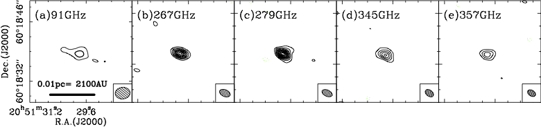 Figure 1
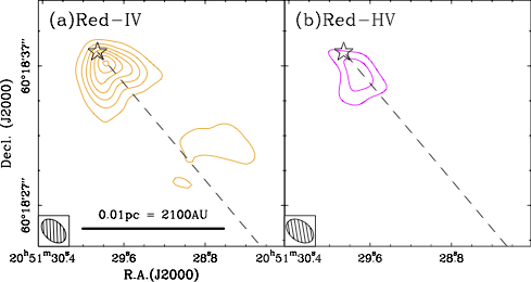 Figure 2
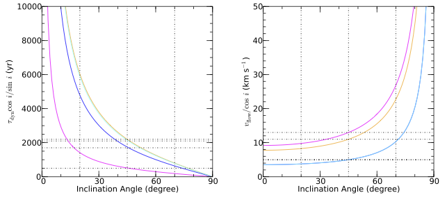 Figure 3
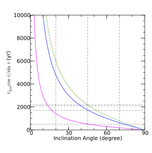 Figure 4
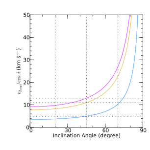 Figure 5
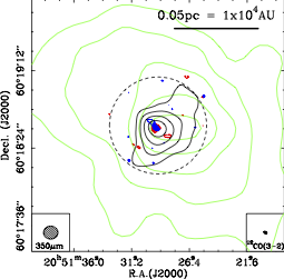 Figure 6
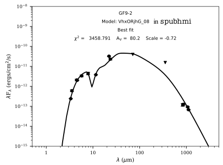 Figure 7
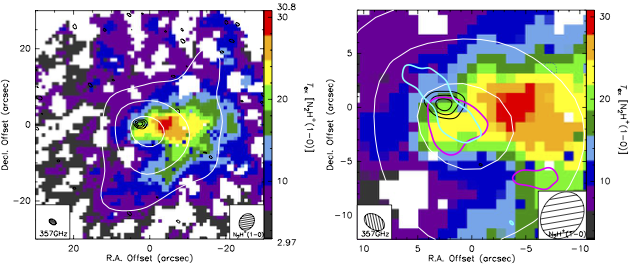 Figure 8
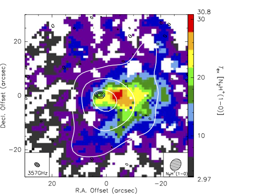 Figure 9
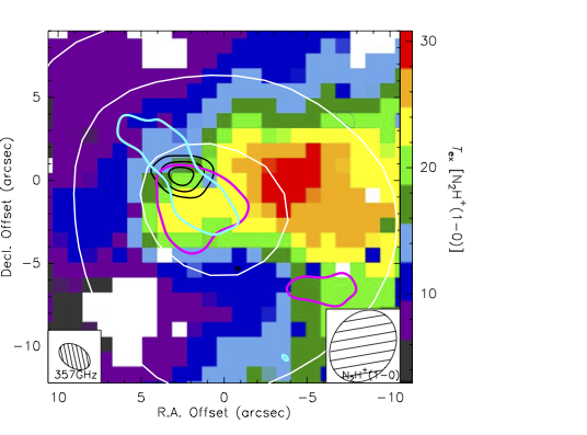 Figure 10
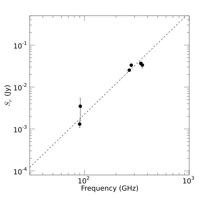 Figure 11
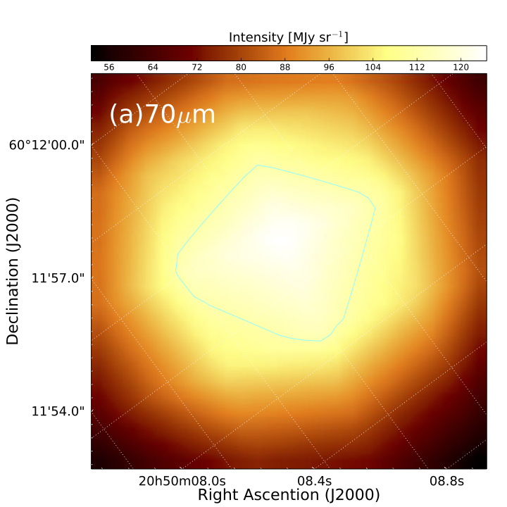 Figure 12
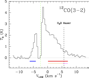 Figure 13
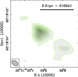 Figure 14
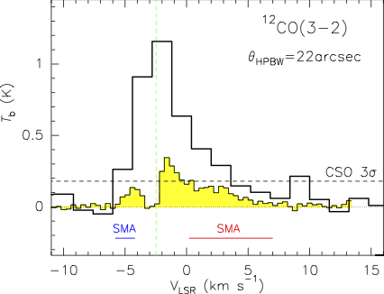 Figure 15
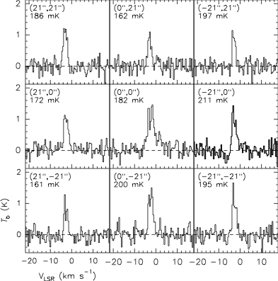 Figure 16
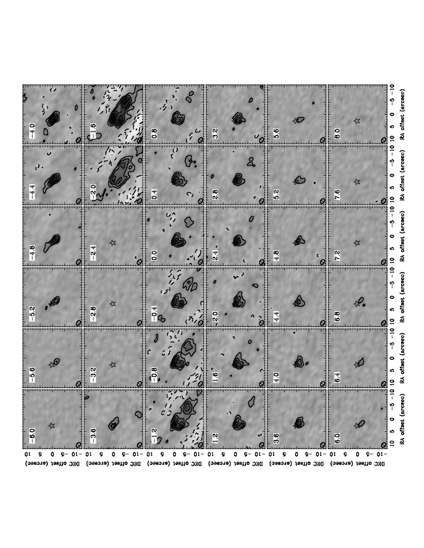 Figure 17
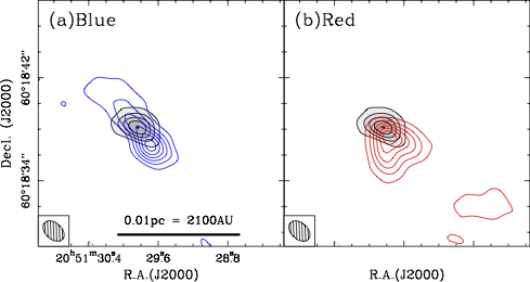 Figure 18
| Spatial Frequency | Synthesized Beam | ||||||||||
|---|---|---|---|---|---|---|---|---|---|---|---|
| Array | Emission | aa Total bandwidth per polarization. | bb Wavelength. | FoVcc Field-of-view. | Range | LASdd Largest detectable angular size scale. | P.A. | Sensitivity | |||
| (GHz) | (MHz) | (mm) | (arcsec) | () | (arcsec) | (arcsec) | (deg) | (mJy beam-1) | |||
| CARMA | Continuum | 91.181 | 938 | 3.29 | 88 | 1.93 – 101.7 | 107 | 3.89 3.34 | 0.32 | ||
| SMA | Continuum | 267.755 | 3960 | 1.12 | 38 | 10.3 – 102.7 | 20 | 2.63 1.61 | 67 | 0.88 | |
| SMA | Continuum | 279.755 | 3960 | 1.07 | 37 | 10.8 – 107.3 | 19 | 2.57 1.14 | 65 | 0.87 | |
| SMA | Continuum | 344.820 | 3960 | 0.869 | 30 | 10.0 – 131.8 | 21 | 2.20 1.43 | 54 | 1.6 | |
| SMA | Continuum | 356.820 | 3960 | 0.840 | 29 | 7.7 – 136.4 | 27 | 2.05 1.34 | 57 | 1.7 | |
| SMA | 12CO(3–2) | 345.796 | 88.4 | 0.867 | 30 | 7.7 – 132.3 | 27 | 2.13 1.39 | 55 | 122ee Sensitivity per velocity channel width of 0.4 km s-1. | |
| Frequency | aa Beam-deconvolved source size obtained by task JMFIT in AIPS package with an assumption that the intensity distribution of the source is approximated by a 2D elliptical Gaussian whose FWHMs along the major and minor axes are and , respectively. | P. A.bb Position angle. | cc Effective source radius in AU. is calculated from where is the distance to the source in pc. The uncertainty is estimated from the difference caused by the elliptical and circular approximations. | dd Peak intensity obtained from the 2D elliptical Gaussian fitting. The error in the fitting is calculated from the RMS noise level of each image (Table 1). | ee Total flux density. | hh “Circumstellar” mass estimated from the values in the column 6. | |
|---|---|---|---|---|---|---|---|
| 2D Gaussianff obtained from the 2D elliptical Gaussian fitting by deconvolving the synthesized beam (see Table 1.). | 3gg obtained by integrating the emission over the area enclosed by the 3 level contour. | ||||||
| (MHz) | (arcsecarcsec) | (degree) | (AU) | (mJy beam-1) | (mJy) | (mJy) | () |
| 89964ii Continuum image was taken from Paper I. All the values are obtained from the re-analysis with the same method as that of the other band data. | 6.62 4.80 | 14015 | 680150 | 1.060.52 | 1.30.23 | 0.710.02 | 0.0520.09 |
| 91181 | 7.56 2.75 | 9515 | 550450 | 1.621.0 | 3.51.9 | 1.230.28jj Except for the weak emission elongated to the east (see Figure 1a). | 0.130.07 |
| 267755 | 2.60 1.61 | 713 | 25050 | 25.21.6 | 25.20.87 | 229 | 0.0190.006 |
| 279755 | 2.46 1.71 | 614 | 25050 | 29.61.7 | 33.22.0 | 3012 | 0.0220.001 |
| 344820 | 2.87 1.43 | 543 | 240110 | 28.62.5 | 36.63.4 | 349 | 0.0120.001 |
| 356820 | 2.59 1.80 | 8112 | 26090 | 19.72.7 | 33.45.2 | 246 | 0.0100.002 |
| aa Outflow lobe length calculated from the measured lobe length seen in Figures 9 and 10. Hence we corrected for the unknown inclination angle of the outflow axis () by assuming . | P.A.bb Outflow lobe position angle measured by eye. The uncertainty is typically 10°. | cc Outflow lobe opening angle measured by eye. The uncertainty is typically 30°. | dd Outflow velocity given by . | ee Dynamical time scale given by . | ff Outflow lobe mass obtained by the 12CO integrated intensity over the velocity range defined in §3.3.4. The left and right column values correspond to the masses in the cases of 7.3 K and 22.6 K, respectively. | gg Outflow mass loss rate estimated by . | hh Outflow momentum rate estimated by . | ii Outflow mechanical luminosity estimated by . | ||||||||
|---|---|---|---|---|---|---|---|---|---|---|---|---|---|---|---|---|
| Lobe | 7.3 K | 22.6 K | 7.3 K | 22.6 K | 7.3 K | 22.6 K | 7.3 K | 22.6 K | ||||||||
| (AU) | (deg) | (deg) | (km s-1) | (yrs) | () | ( yr-1) | ( yr-1 yr-1) | ( ) | ||||||||
| Blue: Northeast | 1600 | 5 | 2000 | 1.2 | 0.14 | 5.5 | 0.71 | 2.9 | 0.37 | 1 | 2 | |||||
| Blue: Southwest | 1300 | 5 | 1700 | 2.2 | 0.28 | 13 | 0.17 | 6.8 | 0.88 | 3 | 4 | |||||
| Red: IV | 3600 | 11 | 2100 | 44 | 5.6 | 200 | 26 | 230 | 30 | 2 | 0.3 | |||||
| Red: HV | 1000 | 13 | 500 | 17 | 0.22 | 34 | 4.4 | 46 | 5.9 | 0.5 | 6 | |||||
| Wavelength | Camera | Aperture | |
|---|---|---|---|
| (µm) | (arcsec) | (mJy) | |
| 350 | SHARC-II | 8.4 | aa Considered to be an upper limit because the aperture is significantly larger than the source size. |
| 70 | MIPS | 18.0 | aa Considered to be an upper limit because the aperture is significantly larger than the source size. |
| 24 | MIPS | 6.0 | 184.0cc Photometric uncertainties in Spitzer images are typically 10%. |
| 22.09 | WISE4 | 12.0 | dd Photometry at the WISE bands are taken from those for WISE J205129.83+601838 in the WISE All-Sky Release Source Catalog. |
| 11.56 | WISE3 | 6.5 | dd Photometry at the WISE bands are taken from those for WISE J205129.83+601838 in the WISE All-Sky Release Source Catalog. |
| 8.0 | IRAC | 1.98 | 11.7cc Photometric uncertainties in Spitzer images are typically 10%. |
| 5.8 | IRAC | 1.88 | 6.4cc Photometric uncertainties in Spitzer images are typically 10%. |
| 4.60 | WISE2 | 6.4 | dd Photometry at the WISE bands are taken from those for WISE J205129.83+601838 in the WISE All-Sky Release Source Catalog. |
| 4.5 | IRAC | 1.72 | 3.1cc Photometric uncertainties in Spitzer images are typically 10%. |
| 3.6 | IRAC | 1.66 | 0.72cc Photometric uncertainties in Spitzer images are typically 10%. |
| 3.35 | WISE1 | 6.1 | dd Photometry at the WISE bands are taken from those for WISE J205129.83+601838 in the WISE All-Sky Release Source Catalog. |
| Property | Symbol | Unit | Resultsaa See Figure 13. The best-fit model is g5QAQXBF_07 in the model set of spubhmi. |
|---|---|---|---|
| Stellar radius | 3.7 | ||
| Stellar surface temperature | K | 3400 | |
| Disk mass [dust] | |||
| Disk outer radiusccfootnotemark: | AU | 50 | |
| Disk flaring power | 1.1 | ||
| Disk surface density power | |||
| Disk scaleheight | AU | 3.7 | |
| Envelope density [dust] | g cm-3 | ||
| Cavity density [dust] | g cm-3 | ||
| Cavity opening angle | deg | 20 | |
| Cavity power | 1.4 | ||
| Inclination angle | deg | 65 |
Peer Reviews
No public reviews on file for this paper yet. If you reviewed it on a platform where reviews are public (OpenReview, ICLR, NeurIPS, ICML), you can paste yours below so the community can read it here.
Videos
No videos yet. Explain this paper in a talk, walkthrough, or lecture? Add one.
A 1000 AU Scale Molecular Outflow Driven by
a Protostar with an age of \mathrel{\hbox{\hbox to0.0pt{\hbox{\lower 4.0pt\hbox{\sim}}\hss}\hbox{<}}}4000 Years
Ray S. FURUYA
Institute of Liberal Arts and Sciences, Tokushima University, Minami Jousanjima-Machi 1-1, Tokushima, Tokushima 770-8502, Japan
Yoshimi KITAMURA
Institute of Space and Astronautical Science, Japan Aerospace Exploration Agency, Yoshinodai 3-1-1, Chuo-ku, Sagamihara, Kanagawa 252-5210, Japan
Hiroko SHINNAGA
Chile Observatory, National Astronomical Observatory of Japan, Current address: Department of Physics, Faculty of Science, Kogoshima University, Korimoto 1-21-35, Kagoshima, Kogoshima 890-0065, Japan
Abstract
To shed light on the early phase of a low-mass protostar formation process, we conducted interferometric observations towards a protostar GF 9-2 using the CARMA and SMA. The observations have been carried out in the 12CO line and in the continuum emission at the wavelengths of 3.3 mm, 1.1 mm and 850 µm with a spatial resolution of AU. All the continuum images detected a single point-like source with a beam-deconvolved effective radius of 25080 AU at the center of the previously known 1.1 – 4.5 molecular cloud core. A compact emission is detected towards the object at the Spitzer MIPS and IRAC bands as well as the four bands at the WISE. Our spectroscopic imaging of the CO line revealed that the continuum source is driving a 1000 AU scale molecular outflow, including a pair of lobes where a collimated “higher” velocity ( km s*-1* with respect to the velocity of the cloud) red lobe exists inside a poorly collimated “lower” velocity ( km s*-1*) red lobe. These lobes are rather young (dynamical time scales of 500 – 2000 yrs) and the least powerful (momentum rates of
km s*-1* yr*-1* ) ones so far detected. A protostellar mass of M_{\ast}\mathrel{\hbox{\hbox to0.0pt{\hbox{\lower 4.0pt\hbox{\sim}}\hss}\hbox{<}}}\,0.06 was estimated using an upper limit of the protostellar age of
\tau_{\ast}\mathrel{\hbox{\hbox to0.0pt{\hbox{\lower 4.0pt\hbox{\sim}}\hss}\hbox{<}}}(4\pm 1)\times 10^{3} yrs and an inferred non-spherical steady mass accretion rate of yr*-1*. Together with results from an SED analysis, we discuss that the outflow system is driven by a protostar whose surface temperature of K, and that the natal cloud core is being dispersed by the outflow.
ISM: evolution — ISM: jets and outflows — ISM: individual (GF 9–2, L 1082C, WISE J205129.83+601838 (catalog )) — submillimeter: ISM — stars: formation — stars: protostars
††facilities: SMA, CARMA, OVRO mm-array, Spitzer Science Telescope, CSO 10.4 m telescope
1 Introduction
1.1 Background
Because of the prominent progress in observational and theoretical studies over the past decades, the early phases of the formation of an isolated low-mass star are now certainly well understood. Nevertheless, our knowledge of its earliest phase is obviously limited in the observational studies. The theoretical studies in the late 1960s and the 1970s indicated that, once a cloud core lost support against the collapse due to its self-gravity, the core collapses isothermally in a runaway fashion, which is followed by an accretion process onto a protostellar core. The first kernel of a mass produced at the center of the collapsing cloud core is believed to evolve towards a hydrostatic object which becomes opaque to the dust continuum emission, and thus the cooling by the dust emission becomes inefficient. Such an adiabatic hydrostatic core is referred to as a first hydrostatic core, a first core (Larson, 1969). The thermal evolution of first cores has been extensively studied by e.g., Masunaga et al. (1998) who performed 1D radiative hydrodynamic calculations to track their evolution. Once the central temperature is elevated to about 2000 K, corresponding to the volume mass density of g cm*-3*, molecular hydrogen commences being dissociated into atomic hydrogen. The dissociation uses the thermal energy which originates from the released gravitational energy due to the accretion. After the dissociation is completed, a second hydrostatic core forms. The second cores are believed to correspond to the protostars observed as “class 0” objects (André et al., 1993). Although feasibility of detecting the first cores have been long discussed (e.g., Boss & Yorke, 1995; Omukai, 2007; Tomisaka & Tomida, 2011; Commerçon et al., 2012; Tomida et al., 2013), it is an enormously difficult task for observers to identify the first cores simply because they are very short-lived objects.
Despite such difficulty, the growing numbers of the first core candidates have been reported (e.g., Belloche et al., 2006; Enoch et al., 2010; Chen et al., 2010; Dunham et al., 2011; Pineda et al., 2011; Tsitali et al., 2013; Pezzuto et al., 2012; Hirano & Liu, 2014; Friesen et al., 2014; Maureira et al., 2017) based on unbiased surveys which observed the thermal dust continuum emission at submillimeter (submm) to infrared (IR) bands with space telescopes together with bolometer cameras on ground-based millimeter (mm) to submm telescopes. The theoretical studies predicted that the duration of the first core phase should continue at most a few times yrs which is an order of magnitude shorter than the lifetime of the class 0 objects (e.g., André et al., 2000). Therefore only a handful of the first core objects should exist in nearby molecular clouds when we consider the number of the class 0 sources identified so far and the relative duration between the first and second core phases (Masunaga et al., 1998; Masunaga & Inutsuka, 2000). Therefore the number of the candidates is too many to be consistent with this statistical argument. This raises a question that some of the candidates may have been misidentified and/or the duration of the first cores may be longer than the theoretical predictions. We therefore believe that it is still required to identify protostars at its early evolutionary stage, and study their physical properties.
1.2 Previous Observations
In this context, we performed a detailed study of the natal cloud core harboring an extremely young low-mass protostar GF 9-2 at a distance () of 200 pc (Wiesemeyer, 1997, see a summary in Poidevin & Bastien 2006) located in the GF 9 filament (Schneider & Elmegreen, 1979). The filament was studied by near-infrared (NIR) extinction (Ciardi et al., 1998), and optical and NIR absorption polarization (Poidevin & Bastien, 2006) observations. Poidevin & Bastien (2006) showed that there exist well aligned pc-scale magnetic fields whose overall direction appears to be almost perpendicular to the filament, and discussed that the magnetic fields must have regulated the formation and evolution of the filament. In the filament there are almost equally spaced seven dense cloud cores traced by the NH3(1,1) lines (Furuya et al., 2008, hereafter Paper II).
Subsequently, Furuya et al. (2014) [hereafter Paper IV] studied the physical properties of the tenuous ambient gas surrounding the dense cloud core GF 9-2 by observing the 1–0 transitions of 12CO, 13CO and C18O molecules, which covered one-fifth of the whole filament. We found that the filament around the core is supported by turbulent and magnetic pressures against self-gravity, and argued that the core has formed through gravitational collapse triggered by the local decay of the supporting force(s).
The cloud core GF 9-2 has been studied in various molecular lines by many authors. Using the NIR extinction map together with the 13CO (1–0) and CS (2–1) line data, Ciardi et al. (1998, 2000) identified an –11 molecular clump of the “GF 9-Core” with a size of 0.8 pc0.6 pc, which harbors the dense cloud core of our interests, a protocore of the “Southwestern Condensation” (Furuya et al., 2014), and the IRAS point source PSC 20503+6006 (see the left panel of Figure 10 in Ciardi et al., 2000). The dense cloud core is cross-identified as L1082 C (e.g., Bontemps et al., 1996; Caselli et al., 2002, and references therein). Caselli et al. (2002) estimated that the core has a mass of 0.350.1 over a radius pc through the N2H+ (1–0) line observations using the FCRAO 14 m telescope (). Figure 2 in Caselli et al. (2002) and Figure 10 in Ciardi et al. (2000) clearly show that the IRAS point source is located at the 90″ (corresponding to 0.08 pc at 200 pc) south-south-west position from the core center. Bontemps et al. (1996) observed the dense cloud core L1082 C, i.e., GF 9-2 in the CO (2–1) line using Caltech Submillimeter Observatory (CSO) 10.4 m telescope () as an outflow survey towards low-mass embedded young stellar objects (YSOs). However, no molecular outflow was detected with the upper limit of 1.5 km s*-1* yr*-1* in outflow momentum rate. In contrast to the negative detection of an outflow, Furuya et al. (2003) detected the H2O maser emission at 22 GHz towards the core center using the Nobeyama 45 m telescope. Although the beam size of the maser observations was (corresponding to 0.072 pc at 200 pc), the presence of the masers strongly suggests that star formation activity has already commenced within a radius of 0.036 pc centered on the cloud core. Subsequently, we carried out higher resolution observations: the N2H+ (1–0) and H13CO+ (1–0) lines using Nobeyama 45 m telescope () and Caltech Owens Valley Radio Observatory (OVRO) millimeter (mm) array (synthesized beam size ) to study the cloud core (Furuya et al., 2006, hereafter Paper I), HCO+ (3–2) line using CSO 10.4 m telescope (25) to detect gas infall in the core (Furuya et al., 2009, hereafter Paper III), and CO (1–0) and (3–2) lines using Nobeyama 45 m (17″) and CSO 10.4 m telescopes (22″), respectively, to assess the negative detection of the outflow (Paper I). Here we scaled the clump mass and size estimated by Ciardi et al. (1998), the cloud core mass and size by Caselli et al. (2002), and the outflow momentum rate by Bontemps et al. (1996) using 200 pc (Wiesemeyer, 1997) because Bontemps et al. (1996); Ciardi et al. (1998, 2000); Caselli et al. (2002) adopted 440 pc. Hereafter, we adopt the distance to the object of 200 pc.
In Paper I, we argued that the central object(s) deeply embedded in the GF 9-2 core has (have) not generated an extensive molecular outflow, as also suggested by Bontemps et al. (1996). The absence of an extensive outflow should provide us with a rare opportunity to investigate the physical properties of the natal core free from the disturbance by the outflow. In Paper III, we reported that “blueskewed asymmetry profiles” in the optically thick HCO+ (1–0), (3–2), and HCN (1–0) lines were detected within a radius of (corresponding to 0.03 pc) suggestive of the presence of large-scale gas infall. The estimated infall velocity was shown to have reasonable consistency with the predictions from the runaway collapse model in the accretion phase (Larson, 1969; Penston, 1969; Hunter, 1977; Whitworth & Summers, 1985, hereafter the LPH solution), and an
infall
rate of yr*-1* was deduced (Paper III). On the other hand, analyzing the N2H+ (1–0) and H13CO+ (1–0) line images that were produced by combining the visibility data taken with the OVRO mm-array and the 45 m telescope, we revealed that a density profile of holds over the annulus of 0.003 \mathrel{\hbox{\hbox to0.0pt{\hbox{\lower 4.0pt\hbox{\sim}}\hss}\hbox{<}}}\,r/\mathrm{pc}\mathrel{\hbox{\hbox to0.0pt{\hbox{\lower 4.0pt\hbox{\sim}}\hss}\hbox{<}}}\, 0.08. Considering possible effects by a putative binary system which was suggested by the positional difference between the 3 mm continuum source and the peak position of the N2H+ emission (; Paper I), we set an inner radius for the region showing the profile to be 0.006 pc. This inner radius gives an upper limit of the protostar’s age of t_{\mathrm{protostar}}\mathrel{\hbox{\hbox to0.0pt{\hbox{\lower 4.0pt\hbox{\sim}}\hss}\hbox{<}}}5\times 10^{3} yrs (Paper I). All the results strongly suggest that the GF 9-2 core has undergone gravitational collapse from the initially unstable state, and has just formed a protostar(s) in the past \mathrel{\hbox{\hbox to0.0pt{\hbox{\lower 4.0pt\hbox{\sim}}\hss}\hbox{<}}}5\times 10^{3} yrs in its center. In order to assess whether or not the protostar has launched a compact molecular outflow(s) and to search for its driving source(s), we performed interferometric observations of the central region of the core in the 12CO (3–2) line and continuum emission.
2 Observations and Data Retrieval
To resolve the issues summarized in §1, we carried out mm- and submm- wavelength interferometric observations with the Combined Array for Research in Millimeter-wave Astronomy (CARMA)111 Support for CARMA construction was derived from the Gordon and Betty Moore Foundation, the Kenneth T. and Eileen L. Norris Foundation, the James S. McDonnell Foundation, the Associates of the California Institute of Technology, the University of Chicago, the states of California, Illinois, and Maryland, and the National Science Foundation. CARMA development and operations were supported by the National Science Foundation under a cooperative agreement, and by the CARMA partner universities. (§2.1) and the Submillimeter Array (SMA)222 The Submillimeter Array is a joint project between the Smithsonian Astrophysical Observatory and the Academia Sinica Institute of Astronomy and Astrophysics and is funded by the Smithsonian Institution and the Academia Sinica.(§2.2), respectively. All the key parameters of the continuum and molecular line emission observations are summarized in Table 1. Note that the SMA observations at wavelengths of 840 µm and 1.1 mm, respectively, provided us with 2.0 and 1.8 times higher angular resolution images than the CARMA did at 3.3 mm, while the CARMA 3.3 mm observations gave us 3.0 and 2.3 times larger fields of view (FoV) and could detect 5.4 and 4.0 times larger spatial structures than the SMA 840 µm and 1.1 mm observations, respectively.
In addition, we used archival Spitzer Space Telescope333 This work is partially based on the data taken with Spitzer Space Telescope, which is operated by the Jet Propulsion Laboratory, California Institute of Technology under a contract with NASA. and Wide-field Infrared Survey Explorer444This publication makes use of data products from the Wide-field Infrared Survey Explorer, which is a joint project of the University of California, Los Angeles, and the Jet Propulsion Laboratory/California Institute of Technology, funded by the National Aeronautics and Space Administration. data. to verify the presence of mid-infrared to far-infrared emission towards the protostar (§2.3).
2.1 CARMA Observations
The aperture synthesis observations tuned at 91.18 GHz, which is the middle frequency of between the N2H+ (1–0) and HCO+ (1–0) emission, were carried out using the CARMA with C, D, and E configurations (project code: c0296). The visibility data used to produce a 3 mm continuum emission image were obtained by 5, 4, and 5 partial tracks performed in 2009 May, April, and June, respectively. Since our primary goal of the observations is to image these molecular lines by combining with the single-dish data taken with the Nobeyama 45 m telescope (Paper I), we carried out nineteen-field mosaic observations. However, in this paper, we concentrate on discussing the continuum emission, and the line data will be published in another paper.
We used J1849+670 as phase and gain calibrators, and 3C454.3, 3C345, J1642+689, and J1751+096 as passband calibrators. The flux densities of J1849+670 were determined from observations of Mars and MWC 349. The uncertainties of our flux calibration were estimated to be approximately . The visibility data were calibrated and edited using the MIRIAD package. For the continuum data, we merged the visibilities in both of the sidebands to improve the image sensitivity: the representative frequency of the continuum image was set to be the center frequency of the dual bands. The image construction was done using the MIRIAD package.
2.2 SMA Observations
The aperture synthesis observations were made using the SMA at the wavelengths () of 1.1 mm and 840 µm on 2010 August 10 and 11, respectively (project code: 2010A-S56). The observations were in the Compact-North configuration using the eight and six antennas at 1.1 mm and 840 µm, respectively. During the observations, the optical depth of the terrestrial atmosphere at 225 GHz ( 1.3 mm) measured with the CSO monitor was fairly stable () except for the last three hours in the dawn of the first night (). The center frequencies of receivers were tuned at 279.5 GHz and 356.7 GHz to receive not only the continuum emission but also molecular lines such as 12CO (3–2), N2H+ (3–2) and HCO+ (4–3) at the 840 µm band as well as HCO+ (3–2) at the 1.1 mm band. Note that the N2H+ and HCO+ lines are typical high-density gas tracers. We configured the correlator so that we can utilize the maximum bandwidth of 4 GHz in each polarization for the continuum detection.
For phase and amplitude calibrators, we observed 3C 418 and BLLac, whose angular distances to the source are 9.2 and 21 degrees, respectively, every 5 minutes. The calibration of the passband response function was done by observing 3C 279, 3C 454.3, 3C 345, and 3C 84 at the beginning and ending of the observations. The scale factors for converting into the absolute flux densities were determined by observations towards Neptune and Uranus. All the visibility data were calibrated and edited using the MIR package. Image construction was subsequently done with the MIRIAD package. For the continuum emission data, we produced an image at each sideband by concatenating the dual polarization data.
2.3 Spitzer Space Telescope Archive Data
We retrieved infrared (IR) images towards the 3 mm continuum source (Paper I) from the Spitzer Science Center data archive. These images are taken at wavelengths of 3.6, 4.5, 5.8, and 8.0 µm taken with the Infrared Array Camera (IRAC; Fazio et al., 2004) (data ID#r26296832), and 24 and 70 µm with the Multiband Imaging Photometer for Spitzer (MIPS; Rieke et al., 2004) (data ID#r26297088) on board the Spitzer Space Telescope.
The point spread function (PSF) sizes of the Spitzer IRAC and MIPS images ranges between 14 at the 3.5 µm band, which are comparable to those in our interferometric observations and 18″ at the 70 µm bands. These fully calibrated data were used without spatial smoothing, and 1 noise levels over emission-free regions are , , , , , and MJy sr*-1* for the 3.6, 4.5, 5.8, 8.0, 24 and 70 µm band data, respectively.
2.4 WISE Archive Data
We retrieved infrared (IR) images towards the 3 mm continuum source from the Wide-field Infrared Survey Explorer (WISE; Wright et al., 2010) data archive. These images are taken at wavelengths of 3.4, 4.6, 11.6, and 22.1 µm. The PSF sizes of the WISE images are at the 3.4, 4.6 and 11.6 µm bands, whereas at the 22 µm band, which are 2–4 times larger than those of the Spitzer images.
3 Results and Analysis
3.1 Continuum Emission at 3.3 mm, 1.1 mm, and 850 µm Bands
In this subsection we describe results obtained from the mm and submm continuum emission maps (Figure 1), which are followed by an analysis of a continuum spectrum (Figure 2).
3.1.1 Maps and Flux Measurements
The 3.3 mm map obtained by CARMA (Figure 1a) was produced by concatenating the visibility data taken at the two sidebands (§2), whereas the 1.1 mm and 850 µm ones by SMA (Figures 1b - e) were produced in each sideband. At all the bands, we detected single point-like sources whose peak positions agree with each other within the spatial resolutions at R. A. , Decl in J2000. In the CARMA 3.3 mm image the object shows a weak elongated structure to the east. No other significant emission was detected over the FoVs (Table 1) at all the bands. This would exclude the “protobinary” hypothesis which we discussed in §5.3 in Paper I.
We performed photometry of the continuum emission using the images at the six frequencies by including the 3.3 mm data analyzed in Paper I.
To estimate the flux densities, we used task JMFIT in AIPS package and IMFIT in CASA to perform beam-deconvolution. Table 2 summarizes our flux density () measurement at each frequency with an assumption that the morphology of the object can be approximated by a 2D elliptical Gaussian. A comparison of the synthesized beam sizes (Table 1) and the beam-deconvolved source sizes (see the values in Table 2) indicates that our observations barely resolved the emission at all the bands, i.e., they are detected as slightly extended sources.
After assessing the beam-deconvolved sizes, we measured the area of the emanating region in the plane-of-sky () to calculate its effective radius () by . For further analysis, we use the mean of 25080 AU calculated from the SMA bands of 1.1 mm and 850 µm because the synthesized beam size () of at SMA observations is better than those at 3 mm.
In order to compare the CARMA 3 mm measurement with the previous one at 3 mm using the OVRO mm-array (; Paper I), we checked consistency between the photometric results from the above Gaussian-fitting method and those measured over the region enclosed by the 3 level contours using the CARMA and SMA data. This is because we adopted the latter method in Paper I. We found a reasonable consistency between the two methods, suggesting that the 2D elliptical Gaussian approximation adopted in the beam-deconvolution processes is reasonable.
3.1.2 Uncertainty in the Flux Measurements
Based on the minimum spatial frequencies of our observations (Table 2) and the discussion in Appendix of Wilner & Welch (1994), we estimated that our SMA observations missed approximately 70% of the flux densities for the extended components of the envelope with respect to the expected zero-spacing flux densities assuming a model with a power-law radial density profile (Paper I).
Table 2 presents the mm- and submm continuum flux densities where we included the previous OVRO measurement (Paper I). We verified that the 3 mm flux difference between the OVRO and CARMA measurement is real. We qualitatively argue that the difference would be caused in the process of synthesis imaging due to the various differences, e.g., those in spatial-frequency () ranges (3.8 67 for OVRO vs. 1.93 101.7 for CARMA) and samplings in the coverage, their weighting functions (the OVRO data were imaged with natural weighting, while the CARMA data with “Robustness of +2”), correlator bandwidths (4096 MHz for OVRO vs. 938 MHz for CARMA), usage of multi-frequency synthesis method in CARMA, and the beam sizes adopted for the photometry (538480 for OVRO vs. 389384 for CARMA). Among these possible causes, we argue that the difference in the ranges may be the most dominant one. However, it is not trivial to explain quantitatively the photometric difference between the OVRO and CARMA results.
3.1.3 Continuum Spectrum over the Millimeter and Submillimeter Bands
Figure 2 presents an interferometric mm- and submm continuum spectrum including the OVRO measurements. Compared to the 1.1 mm and 850 µm flux densities, those at 3.3 mm drop almost one order of magnitude (Table 2; see also Figure 2). Assuming the power-law spectrum with , we obtained the best-fit spectral index of . If we assume that the observed continuum emission at mm and submm regime is fully attributed to optically-thin thermal dust emission represented by a single-temperature graybody emission and that the dust mass absorption coefficient can be written by , the best-fit value obtained between the wavelength range of 3 mm – 850 µm leads to the -index of . The inferred is comparable to those measured at the wavelength range towards circumstellar disks around class II sources (\beta\mathrel{\hbox{\hbox to0.0pt{\hbox{\lower 4.0pt\hbox{\sim}}\hss}\hbox{<}}} 1.0) rather than those measured in molecular clouds, preprotostellar cores, and circumstellar envelope associated with protostars ( 1.5 – 2.0) (e.g., Beckwith et al., 2000; Andrews & Williams, 2007a, b; Ricci et al., 2010a, b; Planck Collaboration, 2011b). Clearly the estimated -index is smaller than those expected for an envelope harboring a protostar. This yields that there might be forming an extremely-dense compact optically-thick region around the protostar or there could still exist a remnant of a first hydrostatic core (e.g., Larson, 1969)(described in §4.5.2).
It is theoretically shown that small dust grains can grow in the innermost densest part of infalling envelopes, e.g., Hirashita & Omukai (2009); Ormel et al. (2011). We therefore estimate mass of the GF 9-2 envelope to infer a mean volume density () to see such a possibility. Assuming that the observed continuum emission is attributed to optically thin thermal dust emission, the total mass of the circumstellar materials, , can be calculated by M_{\mathrm{csm}}$$=\frac{S_{\nu}d^{2}}{\kappa_{\nu}B_{\nu}(T_{\mathrm{d}})} where is the dust mass absorption coefficient at frequency , and the Plank function with dust temperature of . In these calculations, we adopted the usual assumption that has a form of where is a reference value at a reference frequency, . We used the 0.1 cm2 g*-1* at 1.2 THz with 1.8 (Planck Collaboration, 2011b). Notice that the and values lead to of 0.007 cm2 g*-1* which falls between the two values used in Paper I. Moreover we assumed that the dust in the region is well-coupled with the gas. Hence we considered that the excitation temperature () of the N2H+ (1–0) lines (Paper I) represents the gas () and dust () temperatures, i.e., . We adopted the mean excitation temperature of K which is the mean value measured inside the 3 level contour of the 840 µm continuum emission in Figure 1e (Appendix A). We calculated values for the individual bands (Table 2); the mean value of for the higher resolution SMA results and the R_{\mathrm{eff}}$$=25080 AU leads to the order of is cm*-2*. This may be too low for dust grains to coagulate, hence it is unlikely that dust grains over the entire envelope has already grow as in more evolved objects.
3.2 Continuum Emission in the Infrared Image Data
3.2.1 Spitzer data
In Figure 3, we present the Spitzer IRAC and MIPS images centered on the peak position of the SMA 357 GHz source (Figure 1e). Assuming that the absolute positions in the IRAC and MIPS images agree with each other within 036, which is the pixel size common to all the images, these images were “registered” to the 3.6 m one by “reprojecting” using astropy package. Subsequently these images were compared to the SMA images, whose positional accuracies are estimated to be approximately of the synthesized beam sizes of 02 based on the typical errors of the interferometric baseline-vector measurements, angular separations to the calibrators, and their absolute positions. Clearly a point source is detected towards the position of the submm source at all the IR bands. We verified that no other infrared sources are detected within a radius of (corresponding to 0.1 pc) at the 70, 24, and 8 m bands with the detection threshold of the 3 level in each image.
The flux density at each band was computed from the image in unit of MJy sr*-1* with aperture photometry using task apphot in IRAF package with a standard manner; we integrated the emission inside an optimized circle centered on the source after subtracting the background. Notice that the 70 m flux density is considered as upper limits because the HPBWs of the aperture encompassing the source is significantly larger than that of interest for us. The photometry results are summarized in Table 4.
3.2.2 WISE data
Towards the 3 mm continuum source, we clearly detected a point-like source in all the four WISE bands. The object is identified as WISE J205129.83+601838 in the WISE All-Sky Release Source Catalog from which we obtained its Vega magnitudes. These magnitudes were converted into flux densities in unit of Jy (Table 4) with an equation of where is a zero magnitude flux density (Wright et al., 2010) and calibrated WISE Vega magnitudes of the source. The resultant fluxes are shown in Table 4.
3.3 12CO (3–2) Line Emission
Next we present the results from analysis of the SMA 12CO (3–2) line data (Figure 4) and from re-analysis of the previously published 12CO (3–2) line data taken with the Caltech Submillimeter Observatory (CSO)555The Caltech Submillimeter Observatory was operated by the California Institute of Technology under the grant from the US National Science Foundation (AST 05-40882). 10.4 m telescope (Paper I). We also present an overall picture of the data from total integrated intensity map (Figure 5) and interferometric spectrum (Figure 6) where we detected high-velocity wing emission. This forced us to return to checking the single-dish spectra (Figures 7 and 8). After these data inspections, we argue that the CO emission is attributed to a 1000 AU-scale molecular outflow (Figure 9) driven by the continuum source (§3.1 and §3.2).
3.3.1 Velocity Channel Maps
Figure 4 presents velocity-channel maps of the 12CO (3–2) emission taken with the SMA. The blueshifted emission between and km s*-1* is mainly seen towards the southwest of the continuum source, although the emission is much weaker than the redshifted one. Similarly the redshifted emission is also seen towards the southwest, and is detected over a wider velocity range between and km s*-1*. In the velocity channels where the intense emission is detected, e.g., the panels between and km s*-1*, the negative contours are seen along the northeast–southwest direction. We argue that such an artifact is caused by the limited () coverage in our SMA observations.
3.3.2 Spectral Line Profile
Averaging the CO emission along the velocity channel (Figure 4) over the region enclosed by the 3 level contour of the total integrated intensity map (Figure 5), we produced an interferometric 12CO (3–2) spectrum (Figure 6). Here we selected only the bright emission seen in the central peak of Figure 5 to extract the CO emission towards the continuum source. The specific intensity scale in unit of Jy beam*-1* of the spectrum was converted to brightness temperature () in K using the relation of T_{\mathrm{b}}$$=\frac{c^{2}}{2k_{\mathrm{B}}\nu^{2}}\frac{1}{\Omega_{\mathrm{s}}}\int_{\Omega_{\mathrm{s}}}I_{\nu}\mathrm{d}\Omega where is the Boltzmann constant, the light velocity, and the source solid angle. The 12CO (3–2) spectrum taken with SMA shows a noticeable line profile. It has well-defined high velocity wing emission, especially on the redshifted side.
Figure 7 compares the single-dish and interferometric 12CO (3–2) spectra in the scale taken with the CSO 10.4 m telescope (Paper I) and the SMA, respectively. The SMA spectrum was produced by averaging the CO emission inside the CSO beam of (). On the other hand, the previously published CSO data were reprocessed by revising the velocity ranges for the emission-free channels to determine the baseline of each spectrum (Figure 8). Our re-analysis is motivated by the fact that we did not know the presence of the high-velocity wing emission (Figure 6) when we had reduced the data for Paper I. This re-analysis allowed us to detect the redshifted tail emission up to 3.6 km s*-1* and at a single channel centered on 9.2 km s*-1*.
Notice that the high-velocity wing emission is detected only towards the center position (Figure 8).
Using the spectra shown in Figure 7, we computed the integrated intensities of the redshifted emission to be K km s*-1* for the CSO spectrum and K km s*-1* for the SMA one over a velocity range of 0.2\leq$$v_{\mathrm{LSR}}/km s*-1* (described in §3.3.3).
This difference in the total intensity is likely to be caused by the typical uncertainties () in the absolute flux calibrations of the CSO and/or SMA observations, and not by the resolve-out effect in the SMA observations (see the LAS values in Table 1). In other words, the above integrated intensities have not only the thermal noise quoted above but also systematic errors. Contrary to very extended circumstellar envelopes (§3.1), a molecular outflow driven by a protostar in its early stage is generally enough compact to be fully imaged even by the interferometers having small numbers of element antennas (e.g., Arce & Sargent, 2006). We again stress that our CSO observations with the beam detected the redshifted wing emission only toward the center position (Figure 8).
The most straightforward interpretation
for the high-velocity wing emission is that the protostar of interest is driving a molecular outflow. This is simply because the velocity difference between the systemic velocity () and the terminal velocity of the redshifted emission () of |\mbox{v_{\mathrm{t,red}}}-v_{\mathrm{sys}}|\,= 9.5 km s*-1* is
comparable with typical velocities of the outflow lobes observed in low-mass class 0 sources (an order of 1 – 10 km s*-1*; e.g., Bachiller, 1996; Tobin et al., 2016), and is larger than a typical velocity of the envelope gas motions identified as rotation and/or infall (an order of 0.1 – 1 km s*-1*; e.g., Walker et al., 1986; Mardones et al., 1997; Momose et al., 1998). However, the velocity difference on the blueshifted side is moderate: |\mbox{v_{\mathrm{t,blue}}}-v_{\mathrm{sys}}|\,= 3.3 km s*-1*. In this paper, we consider that the blue one is attributed to an outflow system rather than rotation.
Another clear feature seen in the SMA 12CO (3–2) spectrum is that no-emission is seen around the . We consider both or either of the following two causes. One is that the bulk emission near is extended, thus it was resolved out by the interferometer observations. Here the largest detectable angular size scale in our SMA observations was estimated to be 27″ (Table 1), corresponding to 0.026 pc at 200 pc.
Therefore, the extended (\mathrel{\hbox{\hbox to0.0pt{\hbox{\lower 4.0pt\hbox{\sim}}\hss}\hbox{>}}}0.1 pc) low-velocity filament gas (Furuya et al., 2014, see also Figures 8a and b in Paper I) was spatially filtered out by the aperture synthesis observations. The other cause is that the bulk emission around is optically thick, producing a self-absorption trough in the spectrum.
3.3.3 Spatial and Velocity Structures of the Outflow Gas
Next we examine the spatial and velocity structures of the outflow gas unveiled by our SMA 12CO (3–2) line spectroscopic imaging. Figure 9 presents integrated intensity maps of the compact outflow lobes overlaid on the 357 GHz continuum image which has the highest angular resolution among our interferometric continuum images. In order to produce the lobe maps, we defined two LSR-velocity ranges by considering all the features seen in the channel maps (Figure 4) and the spectrum (Figure 6): the blueshifted emission by
and the redshifted emission by .
After defining the LSR-velocity ranges, we calculated a characteristic velocity of each lobe (), which is an intensity weighted mean LSR-velocity, in order to compare with other first core candidates in the literature. This is because the majority of the previous studies which address outflow properties driven by first core candidates and very low luminosity objects preferred to use to represent the flow velocity rather than using the terminal velocity. We therefore calculated v_{\mathrm{ch,blue}}$$=-4.6 km s*-1* in the LSR-velocity for the blue lobe, and v_{\mathrm{ch,red}}$$=+2.5 km s*-1* for the red lobe.
The redshifted lobe is seen to the southwest of the continuum emission, whereas the blueshifted one spreads towards both southwest and northeast. This spatial-velocity structure seen in Figure 9, especially the redshifted one, can be recognized in the early 12CO (3–2) single-dish map taken with the CSO 10.4 m telescope (see Figure 8d in Paper I). However, a caution must be used to compare Figure 8d in Paper I and Figure 9 because the former was obtained for a velocity range of , whereas the latter . Namely, because of the small overlap between the two velocity ranges defined in the CSO and SMA data, we argue that the Figure 8d in Paper I represents mostly the ambient gas, hence we do not consider Figure 8d in Paper I for the discussion about the outflows.
Comparing the spatial extent of the blue and red lobes with that of the 357 GHz continuum emission (see Figure 9), we suggest that the “circum”stellar envelope is, highly likely, being evacuated by the outflow. Such dispersal of the parental gas by outflows has been observed at the core-scale at 0.1 to 0.01 pc with single-dish telescopes (e.g., Monin et al., 1996; Yoshida et al., 2010) and at the envelope-scale with interferometers (e.g., Momose et al., 1996; Velusamy & Langer, 1998; Arce & Sargent, 2006). This is discussed in §4.3.
In the redshifted lobe map, there exist two components (Figure 9b). One is associated with the continuum source (see also the velocity-channel panels of
0.4\mathrel{\hbox{\hbox to0.0pt{\hbox{\lower 4.0pt\hbox{\sim}}\hss}\hbox{<}}}v_{\mathrm{LSR}}/\mbox{km\leavevmode\nobreak\ s{}^{-1}}\mathrel{\hbox{\hbox to0.0pt{\hbox{\lower 4.0pt\hbox{\sim}}\hss}\hbox{<}}}6.8
in Figure 4). The other is (corresponding to AU) southwest of the continuum source, although the latter becomes weak in the higher velocity panels (+1.6\mathrel{\hbox{\hbox to0.0pt{\hbox{\lower 4.0pt\hbox{\sim}}\hss}\hbox{<}}}v_{\mathrm{LSR}}/\mbox{km\leavevmode\nobreak\ s{}^{-1}}\mathrel{\hbox{\hbox to0.0pt{\hbox{\lower 4.0pt\hbox{\sim}}\hss}\hbox{<}}}+3.2) of Figure 4. It is also interesting that the former component shows a fan-shaped structure opened to the southwest (Figure 9b), which is well-recognized especially in the velocity channel panels of 0.4\mathrel{\hbox{\hbox to0.0pt{\hbox{\lower 4.0pt\hbox{\sim}}\hss}\hbox{<}}}v_{\mathrm{LSR}}/\mbox{km\leavevmode\nobreak\ s{}^{-1}}\mathrel{\hbox{\hbox to0.0pt{\hbox{\lower 4.0pt\hbox{\sim}}\hss}\hbox{<}}}+2.8 of Figure 4. Different from the lower velocity fan-shaped redshifted emission, the higher velocity redshifted emission in the velocity range of +5.6\mathrel{\hbox{\hbox to0.0pt{\hbox{\lower 4.0pt\hbox{\sim}}\hss}\hbox{<}}}v_{\mathrm{LSR}}/\mbox{km\leavevmode\nobreak\ s{}^{-1}}\mathrel{\hbox{\hbox to0.0pt{\hbox{\lower 4.0pt\hbox{\sim}}\hss}\hbox{<}}}+6.8 is elongated toward the southwest (Figure 4).
We therefore made another set of outflow lobe maps shown in Figure 10 which presents a comparison of the redshifted intermediate-velocity emission (hereafter “red IV”) integrated over and the redshifted high-velocity emission (hereafter “red HV”) over . These velocity ranges are shown by the horizontal color bars in Figure 6. Note that the “red IV” is composed of the main emission associated with the continuum source and the isolated emission seen to the southwest (see Figure 10a). For the “red IV”, we consider that our observations were not sensitive enough to detect a structure possibly connecting the mainbody and the southwestern island.
Last, we point out an observational fact that the boundary velocity between the “red IV” and “red HV” lobes is close to the LSR-velocity of the H2O maser emission at 22 GHz (Furuya et al., 2003)(see Figure 6). The co-existence of the prominent CO wing emission and the maser transition which is widely believed to be excited in a shocked region (e.g., Hollenbach et al., 1993, 2013; Furuya et al., 2001), strongly suggests that the masers are collisionally excited in the shocked region between the red-IV lobe with the ambient medium (see Figure 6).
In summary,
our SMA observations clearly detected a prominent high-velocity outflow in the CO (3–2) emission towards the central object in the core. Because no other continuum sources are detected, the continuum source must be driving the outflow. The compact outflowing gas has the following features: (i) both the blue and red lobes are bright at the southwest of the continuum source, (ii) bipolarity between the blue- and red lobes cannot be uniquely identified with respect to the continuum source position, (iii) the blue lobe exhibits an elongated structure along the northeast-southwest direction, and (iv)
the red lobe can be resolved into the dual structures of the “red IV” lobe and the “red HV” one. The “red IV” lobe has a wide opening angle,
whereas the “red HV” lobe is more collimated than the “red IV”: the former apparently traces the central axis of the latter.
3.3.4 Physical Properties of the Compact Outflow Lobes
Although the spatial relationship between the outflow lobes and the driving source is puzzling, we derived the physical properties of the lobes: size, position angle (P.A.), opening angle (), flow velocity, dynamical time scale (), mass (), mass loss rate (), and momentum rate (). These parameters are summarized in Table 3.
For the red lobes, we calculated the outflow properties for the “red IV” and “red HV” ones (see Figure 10). We spatially divided the blue lobe into the northeastern and southwestern ones (see Table 3). The two blue lobes are separated by the line of P.A. which passes the peak of the continuum emission. Notice that the two blue lobes are defined over the common LSR-velocity range (§3.3.3).
Adopting the axis lines which pass the continuum peak and have the position angles in Table 3 as reference axes,
we measured the opening angle by eye because it is not easy to uniquely define the lobe shapes. We estimate that the uncertainties in would be 30°.
The dynamical time scale is estimated from the ratio between the maximum extent of the lobe and the flow velocity which is given by (§3.3.2.
; Table 3).
Moreover, because
no information about the outflow inclination is available from observations, we assumed an outflow inclination angle () of .
Here we defined by the angle between the outflow axis and the line of sight.
In order to see the uncertainty caused by the unknown values, we present Figure 11 which shows how outflow velocity and change with outflow inclination angles. We obtained the range from 500 to 2000 yrs for the “red HV” and “red IV” lobes by
correcting for .
Here we did not use calculated in §3.3.3 for the estimates because the use of overestimates the values, which propagate to the other physical properties.
In §3.3.2, we described that the outflow wing emission is detected only towards the center position among all the CSO spectra (see the km s*-1* component in the central panel of Figure 8). Assuming that the 9.2 km s*-1* component represents line-of-sight velocity of a redshifted lobe, we can have another inference of : the beam size for the single-dish 12CO (3–2) observations and the flow velocity given by km s*-1* yields an upper limit of \tau_{\mathrm{dyn}}\mathrel{\hbox{\hbox to0.0pt{\hbox{\lower 4.0pt\hbox{\sim}}\hss}\hbox{<}}}l/v_{\mathrm{flow}}= 900 yrs where l\mathrel{\hbox{\hbox to0.0pt{\hbox{\lower 4.0pt\hbox{\sim}}\hss}\hbox{<}}}(\theta_{\mathrm{HPBW}}/2)/\sin(45\arcdeg)= 3100 AU. The upper limit does not contradict with the range of 500 – 2000 yrs estimated from the interferometric images.
For calculating we assumed that the 12CO wing emission is optically thin and its excitation is in LTE.
We keep using the 12CO/H2 abundance ratio of (Dickman, 1978) for a comparison with previous papers. We adopted the range of the excitation temperature to be between 7.3 K and 22.6 K. Here, the lower limit is given by adding the temperature of the cosmic microwave background emission to the peak brightness temperature of the CO spectrum (Figure 6), whereas the upper limit is the gas temperature described in §3.1. We also measured mean of the gas over the regions enclosed by the 3 contours of the blue- and redshifted lobes to be 20.43.0 K and 17.45.6 K, respectively (Appendix A), both of which fall in the range. Because it is not necessarily certain whether or not the of the N2H+ (1–0) lines, which generally probe a static dense core gas, traces the temperatures of the outflowing gas where the CO transitions are excited, it is reasonable to adopt such a range rather than using a single value.
By integrating the lobe emission shown in Figure 9, we estimated to be of the order of . The lobe masses would be underestimated for the following two reasons. One is that the lobe emission was assumed to be optically thin. The other is the uncertainty in defining the boundary velocities between the outflowing gas and the ambient quiescent gas due to the effect of the resolve-out and/or the self-absorption (§3.3.3). Both the northeastern and southwestern blue lobes have comparable and values. Notice that the majority of the red lobe mass is attributed to the “red IV” one.
After obtaining , the mass-loss, momentum rates, and mechanical luminosity are estimated to be yr*-1*, km s*-1* yr*-1*, and , respectively (Table 3).
The “red IV” lobe is one order of magnitude more powerful than the blue lobes (see in Table 3). In §3.3.3 we pointed out that the spatial extent of the “red HV” lobe corresponds to the central axis of the “red IV” lobe. However, a comparison of their values suggests that the “red HV” lobe is too powerless to drive the “red IV” lobe.
We argue that the outflow lobes in the GF 9-2 core is clearly one of the smallest, the least massive, and the least powerful outflows when we compare with other sources compiled in e.g., Beuther et al. (2002); Takahashi et al. (2008); Takahashi & Ho (2012); Bally (2016).
4 Discussion
4.1 Excluding “Class 0 proto-brown dwarf” and Wide Binary Scenarios
Considering an upper limit of the luminosity reported in the previous work (L_{\mathrm{bol}}$$<0.3; Wiesemeyer, 1997), Palau et al. (2014) categorized this object as a Very Low Luminosity Objects (VeLLOs; see Kauffmann et al., 2005; di Francesco et al., 2007, for definitions) more specifically, a “class 0 proto-brown dwarf”. However, this interpretation may be unlikely because of the “envelope infall rate” with the order of yr*-1* (§4.3) which is certainly larger than the upper envelope of yr*-1* for VeLLOs discussed in e.g., Pineda et al. (2011). It should be noticed that this comparison should be made among infall rates measured in the core-scale at 0.1–0.01 pc, not in the envelope-disk scale at \mathrel{\hbox{\hbox to0.0pt{\hbox{\lower 4.0pt\hbox{\sim}}\hss}\hbox{<}}}10^{2} AU, because majority of the previous works used data obtained with the core-scale.
In the previous work we pointed out that there is a positional offset of 6″ between the 3 mm source and the peak of the N2H+ (1–0) emission (see Figure 15 in Paper I), and proposed that the offset can be interpreted as the presence of a binary system. Clearly such a wide binary scenario is rejected by the higher resolution SMA observations. However, we do have neither positive evidence to support the presence of a closer binary whose separation is smaller than our beam sizes (\mathrel{\hbox{\hbox to0.0pt{\hbox{\lower 4.0pt\hbox{\sim}}\hss}\hbox{<}}}400 AU) nor negative one to reject such a possibility.
Therefore, we keep our assumption that the outflow is driven by a single object to make our discussion as simple as possible.
4.2 Age of the Outflow Driving Source
It should be noticed that the range of dynamical time scale of the outflow lobes (500 – 2000 yrs; §3.3.4; Table 3) is comparable or shorter than those for typical class 0 sources ( – yrs; e.g., Bachiller, 1996; Bontemps et al., 1996; Arce & Sargent, 2006; Curtis et al., 2010; Velusamy et al., 2014). Contrary to the red lobes, the blue lobes seem to be a few times older than the red ones, but their values are still comparable to those of the youngest class 0 sources.
Figure 12 demonstrates the compactness of the outflow system by a comparison of the size scales between the 0.1 pc-scale molecular cloud core and the 1000 AU-scale circumstellar structure, i.e., envelope. Here the cloud core is represented by the H13CO+ (1–0) line whereas the envelope by the 350 µm continuum emission (Paper I). The total extent of the outflow is about of that of the cloud core and is about of that of the envelope when measured along its polar direction (NE-SW), indicating that the central object must be in its early evolutionary stage. Moreover the compactness of the outflow indicates that the outflow has not yet dispersed the parental core. The overall NE-SW direction of the outflow system is almost perpendicular to the elongation of the 350 µm envelope, suggestive of on-going disk-mediated accretion. This orthogonality is not affected by the absolute position accuracy of the 350 µm image (\mathrel{\hbox{\hbox to0.0pt{\hbox{\lower 4.0pt\hbox{\sim}}\hss}\hbox{<}}}4\arcsec; Paper I). Hence, if an edge-on disk exists, its elongation should be almost parallel to that of the envelope.
In addition to the outflow dynamical time scale, we can obtain another constraint on the source age from the size of the free-fall region centered on a forming protostar. Despite the presence of the compact outflow, in the radial column density profile, (Figure 11 in Paper I), we identified that the best-fit power-law profile with an index of holds down to \mathrel{\hbox{\hbox to0.0pt{\hbox{\lower 4.0pt\hbox{\sim}}\hss}\hbox{<}}}600 AU and a free-fall profile with an index of was not recognized in r\mathrel{\hbox{\hbox to0.0pt{\hbox{\lower 4.0pt\hbox{\sim}}\hss}\hbox{>}}}600 AU. Because the gas motions over the core is well described by the extended Larson-Penston’s solution for 0, i.e., the LPH solution (Papers I and III), the absence of an profile, i.e., in volume mass density, in the r\mathrel{\hbox{\hbox to0.0pt{\hbox{\lower 4.0pt\hbox{\sim}}\hss}\hbox{>}}}600 AU region indicates that free-fall region around the protostar has not yet expanded up to the radius of AU, yielding to an upper limit of the central free-fall region (r_{\mathrm{ff}}\mathrel{\hbox{\hbox to0.0pt{\hbox{\lower 4.0pt\hbox{\sim}}\hss}\hbox{<}}}600 AU). Recall that we conservatively adopted r_{\mathrm{ff}}\mathrel{\hbox{\hbox to0.0pt{\hbox{\lower 4.0pt\hbox{\sim}}\hss}\hbox{<}}}1200 AU in Paper I because of the 6″ separation-binary interpretation (§4.1). We now use r_{\mathrm{ff}}\mathrel{\hbox{\hbox to0.0pt{\hbox{\lower 4.0pt\hbox{\sim}}\hss}\hbox{<}}}600 AU and K (§3.3.4), instead of r_{\mathrm{ff}}\mathrel{\hbox{\hbox to0.0pt{\hbox{\lower 4.0pt\hbox{\sim}}\hss}\hbox{<}}}1200 AU and K used in Paper I, the upper limit of the elapsed time since the first kernel of a mass has formed is updated as,
[TABLE]
The revised upper limit is consistent with the dynamical time scales of the red and blue lobes (see Table 3). Last, the r_{\mathrm{ff}}\mathrel{\hbox{\hbox to0.0pt{\hbox{\lower 4.0pt\hbox{\sim}}\hss}\hbox{<}}}600\,\mathrm{AU} does not contradict with the envelope inner radius (corresponding to in Table 5; described in §4.4).
4.3 “Stellar Mass” of the Outflow Driving Source
Next we attempt to estimate the stellar mass using the mass infall rate in the envelope and the stellar age. Considering the two facts that the gas is globally (r\mathrel{\hbox{\hbox to0.0pt{\hbox{\lower 4.0pt\hbox{\sim}}\hss}\hbox{<}}}30\arcsec, i.e., r\mathrel{\hbox{\hbox to0.0pt{\hbox{\lower 4.0pt\hbox{\sim}}\hss}\hbox{<}}}0.029 pc) infalling onto the central object (Paper III) and that the profile
is identified for r\mathrel{\hbox{\hbox to0.0pt{\hbox{\lower 4.0pt\hbox{\sim}}\hss}\hbox{>}}}600 AU (§4.2), the previously estimated global mass infall rate over the core ( yr*-1*) is considered to be valid in the region of 600\mathrel{\hbox{\hbox to0.0pt{\hbox{\lower 4.0pt\hbox{\sim}}\hss}\hbox{<}}}r/[\mathrm{AU}]\mathrel{\hbox{\hbox to0.0pt{\hbox{\lower 4.0pt\hbox{\sim}}\hss}\hbox{<}}}6000. Indeed, the same assumption, i.e., the global infall rate should represent the mass accretion rate onto a stellar core, was adopted in Maureira et al. (2017) when they discuss evolutionary phase of a first core candidate.
However, this spherical infall rate would not hold for the inner r\mathrel{\hbox{\hbox to0.0pt{\hbox{\lower 4.0pt\hbox{\sim}}\hss}\hbox{<}}}\,600 AU region. This is because the compact outflow has already launched, suggestive of non-spherical disk-mediated accretion onto the forming star due to the dispersal of the envelope by the outflow (§3.3.3). Therefore, we take a non-spherical steady accretion rate of for r\mathrel{\hbox{\hbox to0.0pt{\hbox{\lower 4.0pt\hbox{\sim}}\hss}\hbox{<}}}600 AU where an efficiency coefficient is written as with a total solid angle of the blue and red lobes viewed from the central star (). Assuming the shapes of the bipolar outflow lobes are conical, we calculated the total solid angle of the lobes as steradian for the which is the widest opening angle of the “red IV” lobe (Table 3). We obtained , leading to the non-spherical steady accretion rate of,
[TABLE]
Then the object may have acquired a stellar mass of,
[TABLE]
since the formation of the central point source. Here the upper limit in Eq.(4) is due to the upper limit in the estimate [Eq.(2)]. Notice that the value does not change significantly even if one consider the range of the outflow dynamical time scales, , as the age of the object.
We must keep in mind that the current accretion/outflow rates may much differ from the time-averaged rates during the formation process of the possible disk-outflow system or a possibility that an accretion rate from the envelope onto a putative disk should differ from an accretion rate from the disk onto the central object. However, because such more rigorous discussion is beyond the scope of this paper, we assume that the accretion rates onto the disk and the forming star are equal to each other and steady for further discussion.
4.4 Spectral Energy Distribution of the Outflow Driving Source
In order to obtain further constraints on the nature of the source, we produced Figure 13 where spectral energy distribution (SED) of the outflow driving source between the mm bands and Spitzer bands is presented. The model SEDs were obtained by using a sedfitter tool by Robitaille et al. (2006) together with large sets of SED models provided by Robitaille (2017). As emphasized by the author, we have to keep in mind the limitations of the tool and the model sets because they provide simplified SED model sets to search for a first-order-of-approximation picture of a YSO of interests among the various combinations of physical parameters characterizing a YSO. Each model set in Robitaille (2017) allows us to search for the best-fit solution in a wider range of the model parameters than the original one (Robitaille et al., 2006). Each set consists of a protostar or a pre-main sequence (PMS) star surrounded by an accretion disk and a rotationally infalling envelope with a bipolar outflow, and also considers the scattering and reprocessing of the stellar radiation by dust. Moreover, some model sets include a bipolar cavity dispersed by an outflow. In each model set, model SEDs were computed at 10 different viewing angles by convolving a frequency-filter function and an aperture size at each measurement; we used the default ones for the Spitzer measurements, and added those for our CSO, SMA, CARMA, and OVRO observations.
To fit the photometry results (Tables 2 and 4), we set a distance range of 20020 pc, and used an extinction curve by Whitney et al. (2003, 2004), allowing to estimate the foreground as well (see the value in each panel of Figure 13). We dealt with the 70 m flux density as an upper limit because the HPBW of the aperture encompassing the source is much larger than those imaged by SMA, CARMA and OVRO interferometers. Notice that the number of the free parameters in the model sets (see Table 2 in Robitaille, 2017) ranges between 2 and 12, whereas we have fifteen data points (), including the upper limits. A caution must be used for the WISE 22 m and Spitzer 24 m data whose aperture sizes are comparable to that for the 350 m (Table 4). This is because we did not consider them as upper limits because the 22 and 24 m emission most likely comes from the central compact component(s) rather than from the extended envelope traced by the 70 and 350 m emission. Indeed, we found that all the models gave us unrealistic SED fits when we set the 22 and 24 m fluxes as upper limits.
As mentioned above, we attempted all the model sets summarized in Table 2 of Robitaille (2017), and selected the most reasonable models from each model set based on the criterion of . In practice, we rejected the 16 out of 18 model sets in Table 2 of Robitaille (2017) because these model sets failed to reproduce the observed SEDs, whereas the remaining two model sets of spu-smi and spubhmi gave reasonable fits. Here the first character of s in the model-set names denotes that they commonly consider emission from a central star, the second one of p does passive disk, the third u does so-called Ulrich-like envelope (an envelope with radial power-law dependency of outside the centrifugal radius , 1/2 inside; Ulrich, 1976). The fourth b in spubhmi indicates that this model set considers a bipolar-outflow cavity, whereas not in spu-smi. The fifth h indicates that the spubhmi model set leaves radius of the inner hole produced by the outflow as a free-parameter, whereas the fifth s means that the spu-smi adopted a dust-sublimation radius as an inner hole radius. The last two characters of mi indicates that the both model sets commonly considered the ambient medium (m) together with the interstellar dusts (i), as described earlier.
On the basis of the inferred physical parameters, we rejected spu-smi because the stellar radius suggested by the model sets ( ) is too small and the stellar surface temperature ( K) is too high for a protostar (§4.2).
The remaining model sets of spubhmi yields the decent SED fit (Figure 13) with the reasonable physical parameters (Table 5). The model gave plausible values of , and K as well as those characterizing the envelope and disk. The inferred inclination angle of from the two models gives a constraint in our analysis in §3.3.4, and will be discussed in §4.5. In addition, the suggested cavity opening angle of may not contradict with our estimate in Table 3 when we consider the uncertainty of our measurement (; §3.3.4). Last, the inferred value does not affect the estimate of the protostar’s age based on the radial density profile (§4.2).
In conclusion, it is highly likely that we are dealing with an edge-on outflow system driven by a K protostar surrounded by a AU radius disk with an infalling envelope. Moreover, we argue that the outflow system whose lobe axis is almost parallel to the plane of sky may not have completed dispersing its natal cloud core.
4.5 Evolutionary Stage of the Outflow Driving Source: Constraints from the Outflow Properties
The SED analysis suggested that the outflow is viewed almost from its side (see e.g., Figure 7 in Tomisaka & Tomida, 2011). In this subsection, we discuss this geometry along with the outflow properties (§3.3.4).
4.5.1 Terminology of the Outflow Velocity and Inclination Angle
Dependency on the Flow Velocity and Dynamical Timescale
Before addressing the outflow geometries, we must clarify the terminology of the outflow velocities when we compare to those in theoretical studies. Most of the theoretical studies refer to “high velocity” as those having of the order of km s*-1* and “low velocity” as 1 km s*-1* \mathrel{\hbox{\hbox to0.0pt{\hbox{\lower 4.0pt\hbox{\sim}}\hss}\hbox{<}}}v_{\mathrm{out}}\mathrel{\hbox{\hbox to0.0pt{\hbox{\lower 4.0pt\hbox{\sim}}\hss}\hbox{<}}}10 km s*-1* (e.g., Bachiller, 1996). Note that these theoretical velocities are the 3D one. In contrast, observers argue outflow velocities projected onto the line of sight. Furthermore there is no widely accepted unique definition of the velocity range for “high” and “low” velocities even if we limit to discussing outflows traced by low- CO lines. Considering these limitations and the uncertainties in our observations, we do not directly compare observed outflow velocities and
those in numerical simulations. Therefore,
we keep using the words of the IV and HV defined in §3.3.3, and use “lower velocity” and “higher velocity” in a relative sense.
As already seen in Figure 11, 3D flow velocity of and the “real” dynamical time scale of for the four lobes strongly depends on . In addition, the opening angles of the lobes are rather large of with the uncertainties of (Table 3). We therefore discuss two representative cases of the pole-on outflow at and the edge-on one at , as done in e.g., Belloche et al. (2006).
4.5.2 “Pole-on” vs. “Edge-on” Outflows Based on the Outflow Age and the Elapsed Time
of Mass Accretion
A Pole-on Outflow (e.g., )
Figure 11 suggests that the 3D-velocities of the pole-on lobes range from 3 to 9 km s*-1*, leading to the corrected ages of yrs. In the pole-on geometry the large spatial-overlapping between the blue and red lobes together with the absence of the redshifted CO emission to the northeast of the continuum source is explained to some extent. This is because the outflow gas moving away from us along the outflow axis should be obscured by the circumstellar materials.
However, there are two major caveats in the pole-on outflow hypothesis. If the pole-on is the case, all the lobes should show more roundish morphology to form a symmetric roundish lobe pairs, but the “red HV” and blue lobes are elongated. It is also impossible to explain the southwest island (see Figure 9b) along with the pole-on hypothesis.
The other major caveat is that the -corrected values of the order of yrs would be larger than the source age of \tau_{*}\mathrel{\hbox{\hbox to0.0pt{\hbox{\lower 4.0pt\hbox{\sim}}\hss}\hbox{<}}}4\times 10^{3} yrs in Eq.(2). We therefore conclude that a pole-on geometry is unlikely.
An Edge-on Outflow (e.g., 70)
If we are observing an edge-on outflow, the 3D-velocities of the lobes would be approximately 10 – 30 km s*-1* (Figure 11), leading to the lobe ages of \tau_{\mathrm{dyn}}\cos i/\sin i\mathrel{\hbox{\hbox to0.0pt{\hbox{\lower 4.0pt\hbox{\sim}}\hss}\hbox{<}}}1\times 10^{3} yrs. It is well-known that protostars, i.e., class 0 sources, show highly-collimated high-velocity outflows whose dynamical time scale ranges – yrs (e.g., Gueth & Guilloteau, 1999; Santangelo et al., 2015). The inferred age range of the GF 9-2 outflow agrees with the range, and is considered to represent elapsed time of the ongoing accretion process (§4.2). If such an edge-on geometry is the case, all the caveats raised in the pole-on hypothesis, except for the absence of distinct bipolarity, may be resolved. In addition, the spatial overlapping of the blue and red lobes seen to the southwest of the continuum source is also reasonably explained by edge-on outflow lobes with large opening angles of (Table 3).
However, the edge-on hypothesis does not explain why the morphology and velocity structure of the blue and red lobes are not symmetric; we should detect redshifted lobe(s) to the northeast of the continuum source.
Such asymmetry may be explained by “realistic” MHD simulations which includes turbulence (e.g., Matsumoto & Hanawa, 2011).
Keeping all the strong and weak points in mind, it is possible that the central object has experienced its second collapse \tau_{\mathrm{dyn}}\cos i/\sin i\mathrel{\hbox{\hbox to0.0pt{\hbox{\lower 4.0pt\hbox{\sim}}\hss}\hbox{<}}}1\times 10^{3} yrs ago. In this interpretation, the poorly collimated “red IV” lobe (Figure 10) would represent a remnant outflowing gas which is the fossil of a lobe that had been driven by the object when it had been at the first core stage, and the “red HV” lobe (Figure 10) is considered as a fresh lobe currently being driven by the protostar. If this is the case, the dynamical time scale of the “red IV” lobe (500 yrs for ; Figure 11) may be interpreted as the duration of the first core stage. In this interpretation, the small of 0.40.3 (§3.1.3) should be attributed to a remnant of the first hydrostatic core.
4.5.3 Summary of the Subsection
Considering the geometry of the compact outflow lobes in conjunction with the and estimates, we suggest that the outflow geometry is edge-on which reconciles with the results from the SED analysis.
5 Summary
Interferometric observations of the 12CO (3–2) line and the continuum emission at 3.3 mm, 1.1 mm, and 850 µm bands were carried out towards the deeply embedded protostar at the center of the dense molecular cloud core GF 9-2 using CARMA and SMA.
Furthermore we analyzed the and satellite images and the single-dish 12CO (3–2) spectra previously taken with CSO. The main findings of this research are summarized as follows.
At the center of the cloud core, we detected a compact continuum source which is considered to be representing a circumstellar envelope at 1.1 mm and 850 µm bands. The beam-deconvolved effective radius, , of the continuum source was measured to be 25080 AU at the 1.1 mm and 850 µm bands where we attained the linear resolution of AU at the distance of the source (200 pc). 2. 2.
Towards the position of the submm source, an infrared source, designated as WISE J205129.83+601838, is clearly detected at wavelengths between 70 µm and 3.4 µm in the Spitzer MIPS and IRAC images as well as WISE ones. This detection clearly indicates that the object is at a protostar phase. Our SED analysis using the sedfitter tool (Robitaille, 2017) suggested its surface temperature of K and stellar radius of 4 . 3. 3.
Our spectroscopic imaging of the 12CO (3–2) line clearly detected a 1000-AU scale molecular outflow system driven by the continuum source. The system exhibits collimated- and poorly collimated redshifted outflow lobes with the line-of-sight velocities of km s*-1* and km s*-1*, respectively. The blueshifted exhibits a collimated lobe extending both towards the northeast and southwest of the central source. Our analysis showed that the outflow lobes are one of the youngest (dynamical time scales of 500 – 2000 yrs) and the least powerful (momentum rates of km s*-1* yr*-1*) ones so far detected. A comparison between the continuum and outflow maps suggests that the innermost part (r\mathrel{\hbox{\hbox to0.0pt{\hbox{\lower 4.0pt\hbox{\sim}}\hss}\hbox{<}}} 2000 AU) of the envelope is being dissipated by the outflow. 4. 4.
The momentum rate of the collimated red lobe does not suffice to drive the poorly-collimated red one, suggesting that they are driven. Based on the outflow morphology, velocity structure of the lobes, comparisons with outflow models and the results from the SED analysis, we concluded that the outflow axis is not far from parallel to the plane of the sky, i.e., the edge-on geometry. 5. 5.
Although the outflow properties agree with those measured in the VeLLOs and the “Class 0 proto-brown dwarfs”, we excluded such interpretations on the basis of the large spherical infall rate of the order of yr*-1*. We also excluded the wide-binary interpretation based on the previous lower resolution data because only a unresolved (\mathrel{\hbox{\hbox to0.0pt{\hbox{\lower 4.0pt\hbox{\sim}}\hss}\hbox{<}}}400 AU) continuum emission was detected by the interferometric observations. 6. 6.
We argued that it has not passed
\tau_{\ast}\mathrel{\hbox{\hbox to0.0pt{\hbox{\lower 4.0pt\hbox{\sim}}\hss}\hbox{<}}}(4\pm 1)\times 10^{3} years since the protostar formed at the center of the cloud core. This is because a radial volume density profile with a form of , which proves the presence of a freely falling gas towards the central object, was not identified outside the
600 AU region in radius which has a consistency with the disk radius inferred from the SED analysis. The upper limit of the protostellar age suggests that the total mass accreted onto the central object is
M_{\ast}\mathrel{\hbox{\hbox to0.0pt{\hbox{\lower 4.0pt\hbox{\sim}}\hss}\hbox{<}}}0.06 .
Given the uniqueness of the source properties, follow-up high-resolution and high-sensitivity observations along with simulation studies are required towards a more complete understanding of the physics in a low-mass protostar formation process.
The authors sincerely acknowledge the anonymous referee whose comments significantly helped to improve quality of this paper, especially critical comments on the Spitzer data. R. S. F. gratefully acknowledges John M. Carpenter and Andrea Isella for their generous help and discussion at the CARMA observations and the data reduction process. R. S. F. also sincerely thanks Masahiro N. Machida, Tomoyuki Hanawa and Shu-ichiro Inutsuka for fruitful discussion, and Takeshi Inagaki for data analysis with Python. This work was partially supported by the JSPS Institutional Program for Young Researcher Overseas Visits (Wakate Haken) at Subaru Telescope of National Astronomical Observatory of Japan (NAOJ) for R. S. F. and H. S. and the AWA support program at Tokushima University for R. S. F. Data analyses in this work were partly carried out on the computer system operated by Subaru Telescope and that by Astronomy Data Center of NAOJ. The authors gratefully acknowledge all the staff at CARMA, SMA, CSO and the Spitzer Science Center, and the MIR software group at CfA, the AIPS software group at NRAO and the GILDAS software group at IRAM.
Appendix A Excitation Temperature Map of the N2H+ (1–0) Emission
As reported in Paper I, we combined the visibility data of the N2H+ line taken with the OVRO mm-array and the single-dish Nobeyama 45 m telescope (see §3.2.3 and Appendix A in Paper I). Using the the combined data we performed the hyperfine structure analysis of the N2H+ transition (see §4.1. and Appendix B.1 in Paper I). The usage of the hyperfine structure lines has an advantage that one can assess both the and optical depth of the lines with relatively high accuracy. In addition, such a combined image allows us to analyze the spatial structure of the gas with an angular resolution that can be achieved by interferometers and the analysis is free from the “missing flux” problem.
In §3.1, we used the mean excitation temperature of the N2H+ (1–0) emission over a circular region with a radius of 25080 AU centered at the submm source [ K]. The mean value was obtained from the map (Figure 14) which was used to produce the column density map of N2H+ shown in Figure 9b of Paper I.
In addition, we measured the mean of 20.43.0 K for the redshifted outflow lobes, including the southwestern island, and 17.45.6 K for the blue one. Here these values were calculated over the regions inside the 3 level contours of the outflow lobes (see Figure 14b).
The reference list from the paper itself. Each links out to its DOI / PubMed record.
- 1André et al. (1993) André, P., Ward-Thompson, D., & Barsony, M. 1993, Ap J, 406, 122
- 2André et al. (2000) André, P., Ward-Thompson, D., & Barsony, M. 2000, Protostars and Planets IV, 59
- 3André (1996) André, P., Ward-Thompson, D., & Motte, F. 1996, A&A, 314, 625
- 4Andrews & Williams (2007 a) Andrews, S. M., & Williams, J. P. 2007, Ap J, 659, 705
- 5Andrews & Williams (2007 b) Andrews, S. M., & Williams, J. P. 2007, Ap J, 671, 1800
- 6Arce & Sargent (2006) Arce, H. G., & Sargent, A. I. 2006, Ap J, 646, 1070
- 7Bachiller (1996) Bachiller, R. 1996, ARA&A, 34, 111
- 8Banerjee & Pudritz (2006) Banerjee, R., & Pudritz, R. E. 2006, Ap J, 641, 949