The transition from order to disorder in Voronoi Diagrams with applications
Lorenzo Zaninetti

TL;DR
This paper investigates the transition from order to disorder in Voronoi diagrams by perturbing seed points, introducing a new scaling relationship, and applying the model to physical and cosmological structures.
Contribution
It introduces a novel relationship modeling the scaling of the Kiang function with a geometrical parameter in Voronoi tessellations.
Findings
Successful modeling of local structures in ammonia using the Voronoi approach.
Application of the model to cosmic void volumes.
Demonstration of the transition from order to disorder in tessellations.
Abstract
The transition from ordered to disordered structures in Voronoi tessellation is obtained by perturbing the seeds that were originally identified with two types of lattice in 2D and one type in 3D. The area in 2D and the volume in 3D are modeled with the Kiang function. A new relationship that models the scaling of the Kiang function with a geometrical parameter is introduced. A first application models the local structure of sub- and supercritical ammonia as function of the temperature and a second application models the volumes of cosmic voids.
Click any figure to enlarge with its caption.
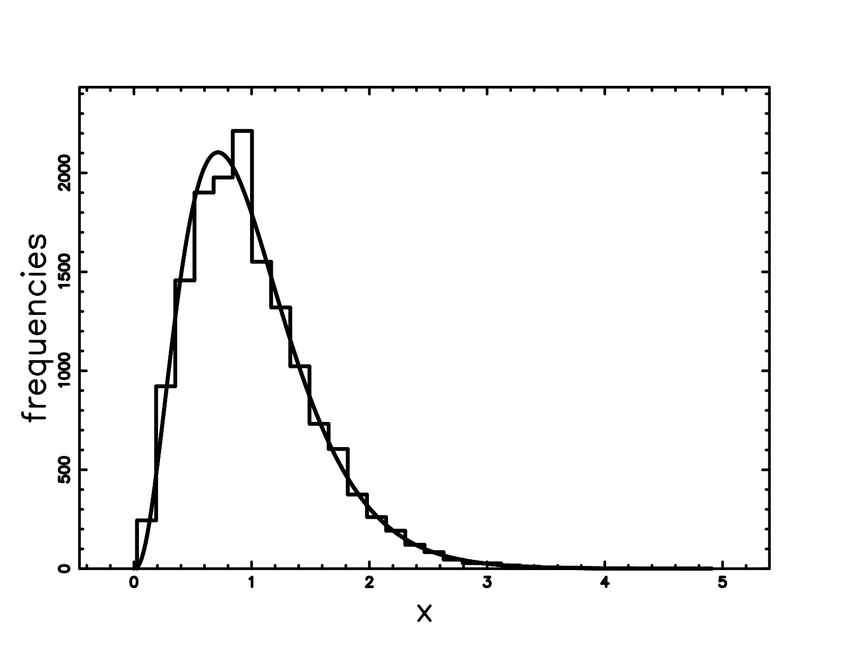 Figure 1
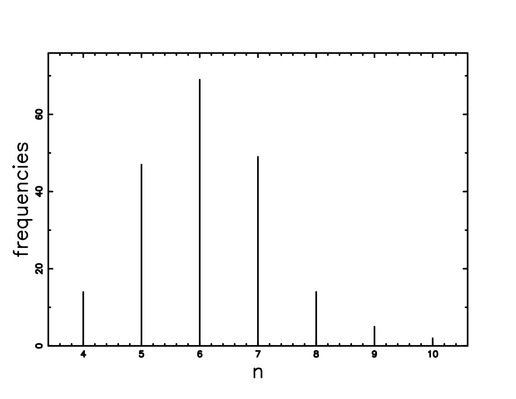 Figure 2
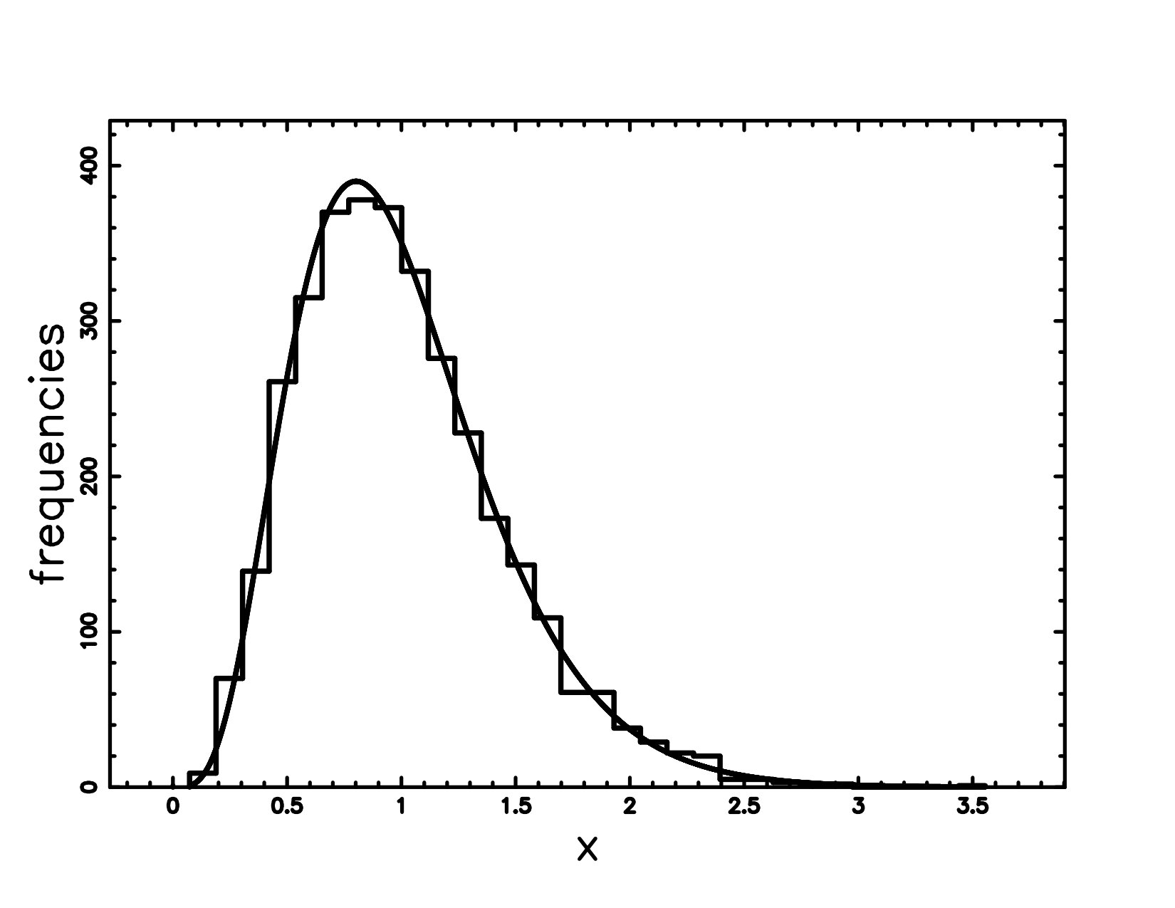 Figure 3
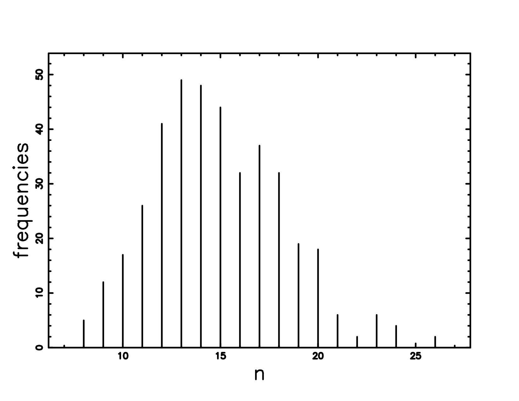 Figure 4
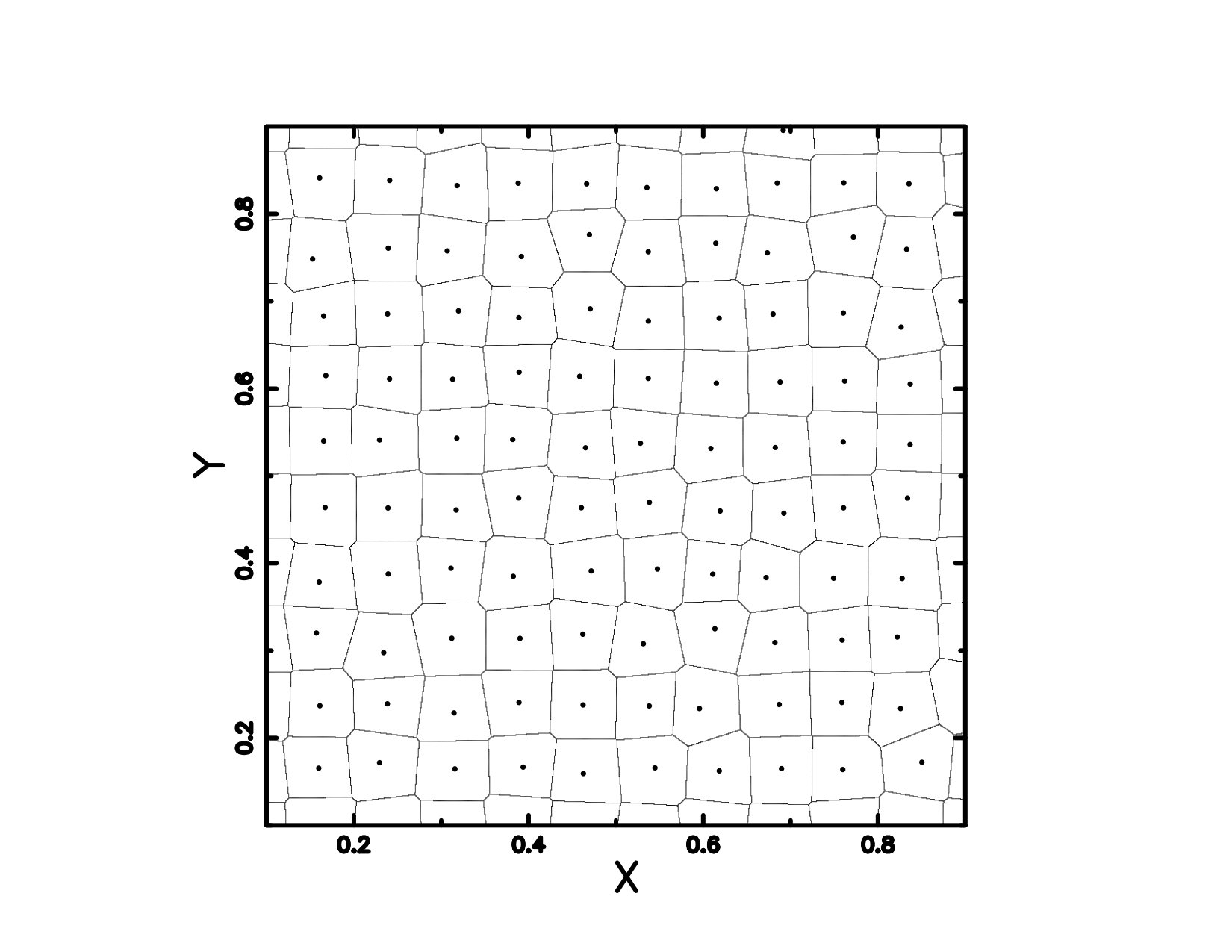 Figure 5
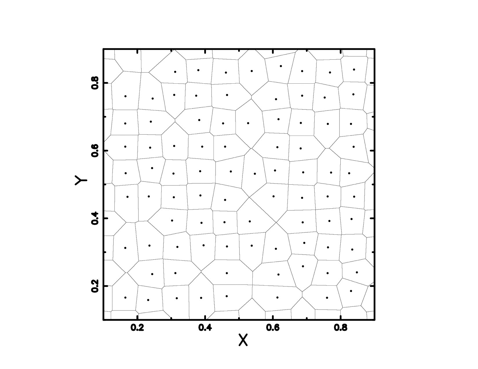 Figure 6
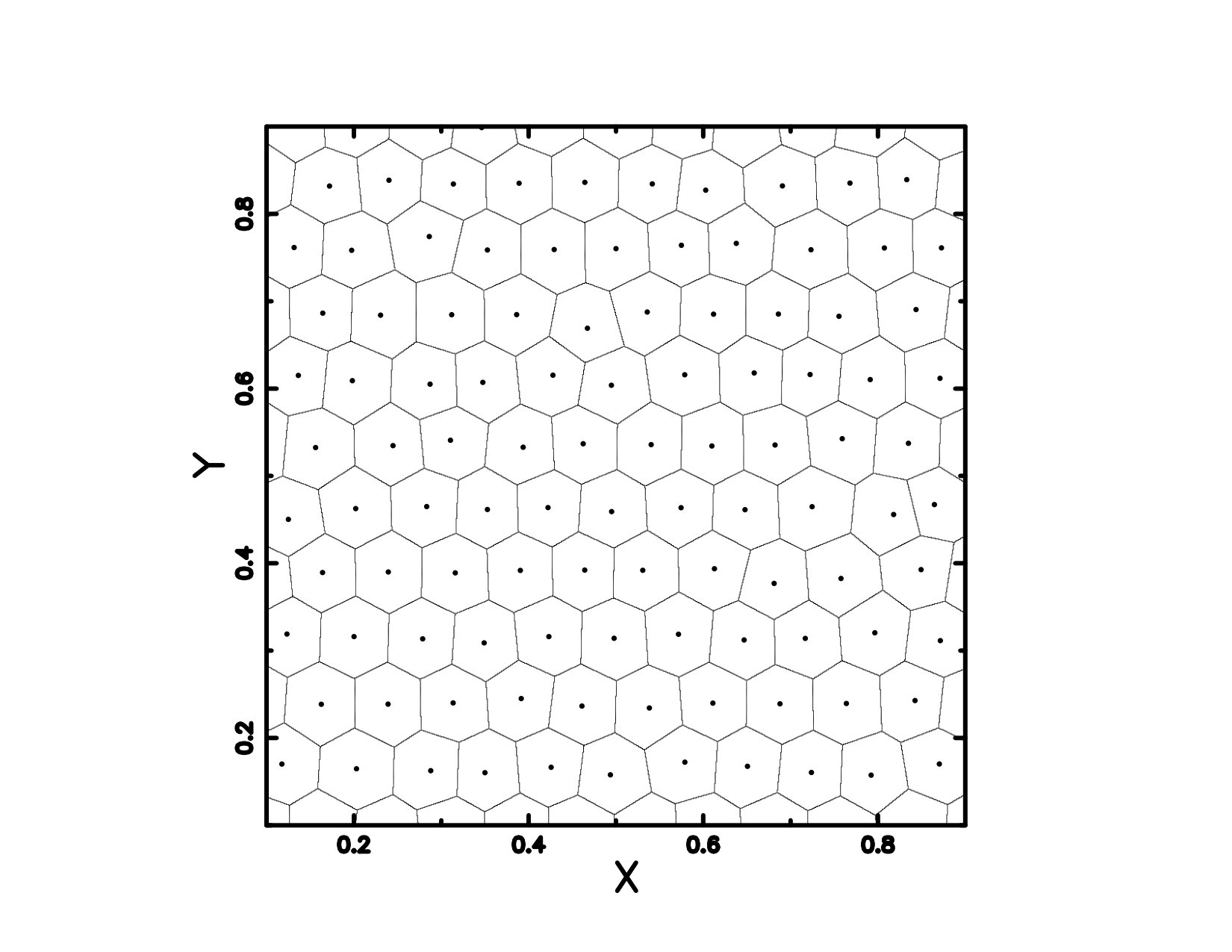 Figure 7
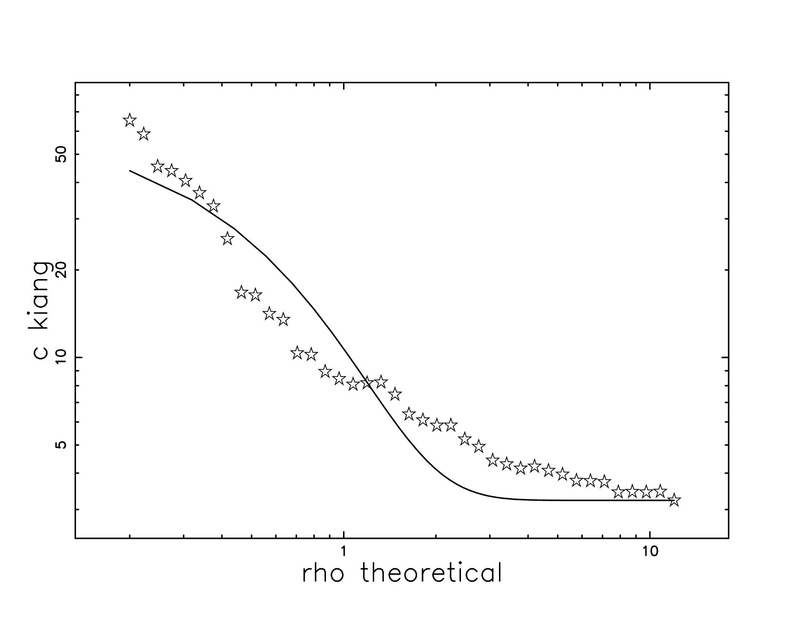 Figure 8
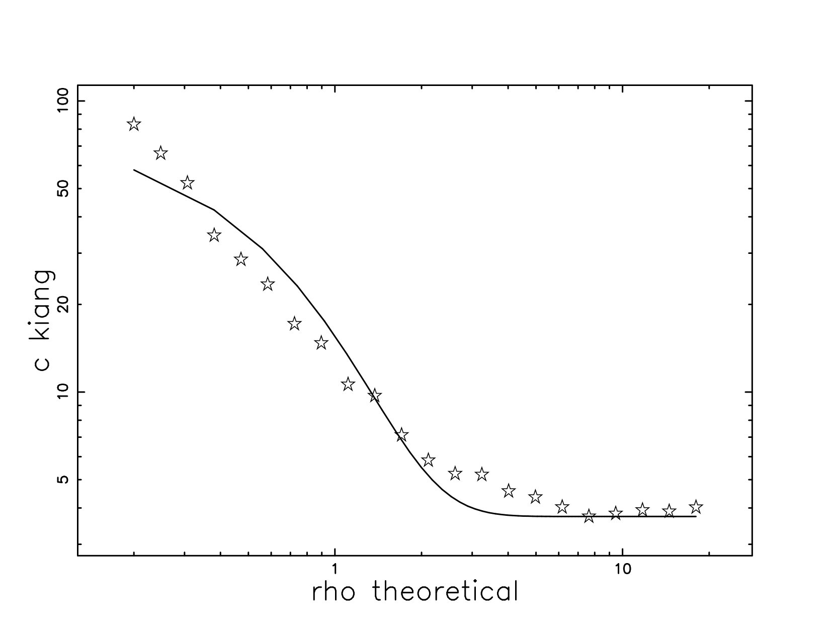 Figure 9
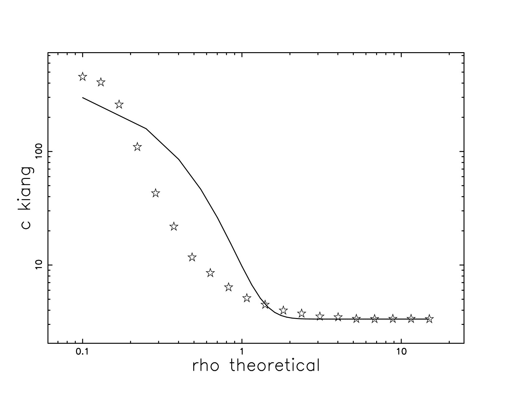 Figure 10
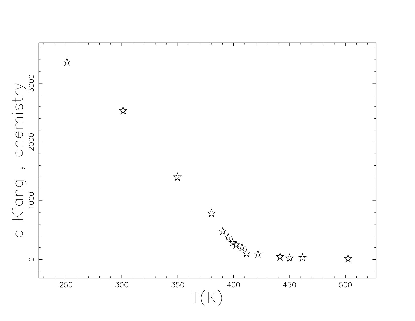 Figure 11
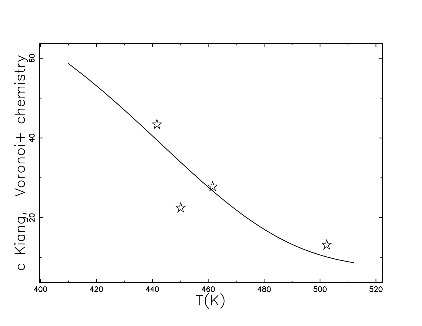 Figure 12
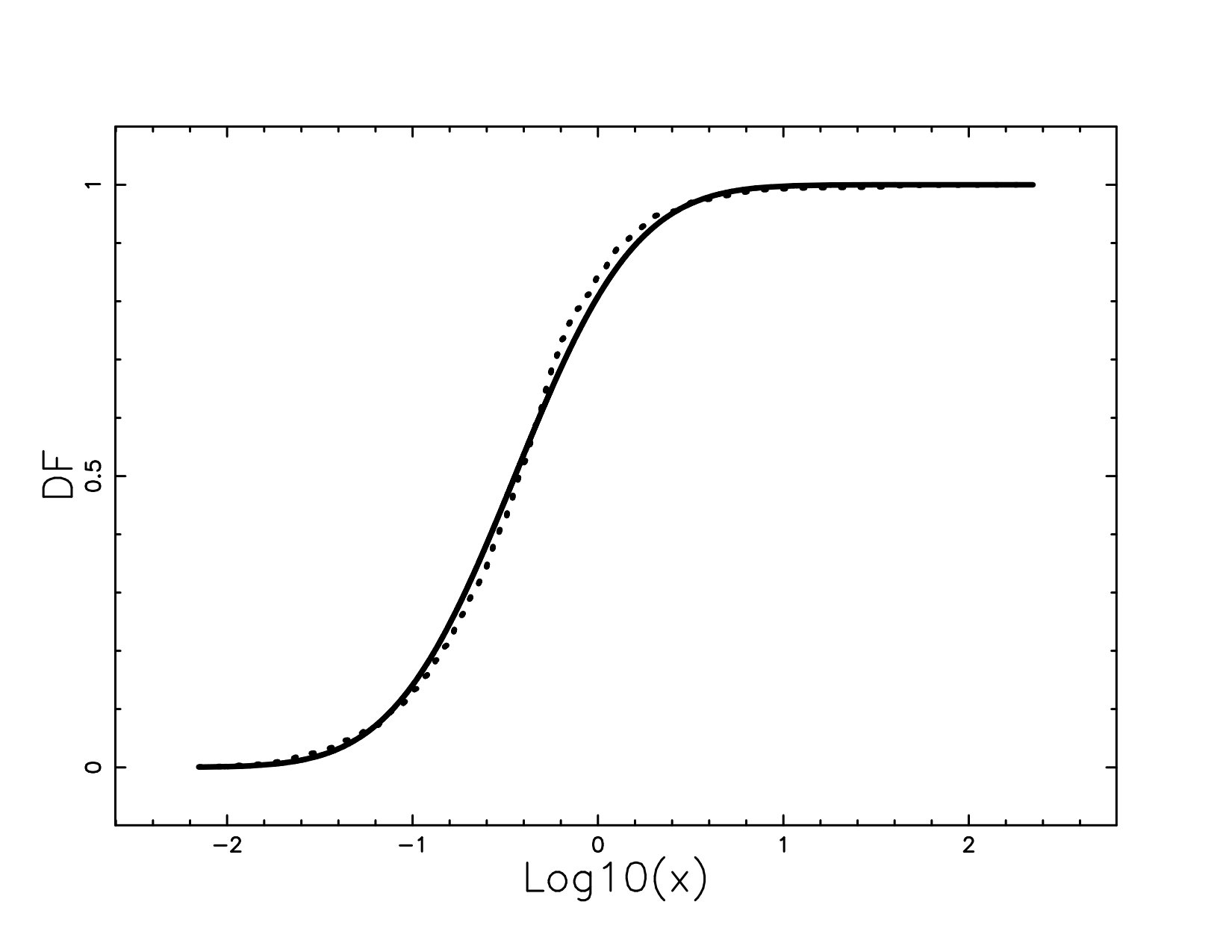 Figure 13
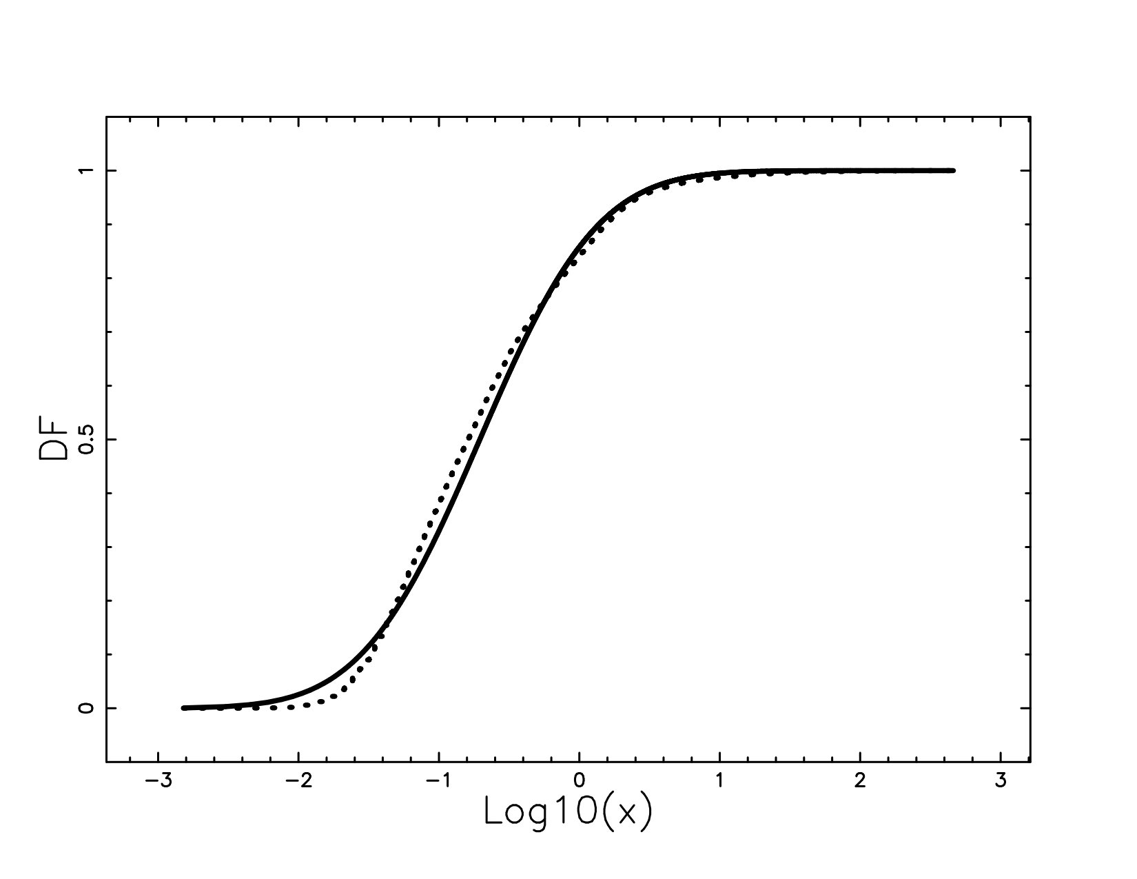 Figure 14
| case | parameters | D | |
|---|---|---|---|
| astronomical observations | ; = 1.182 | 0.049 | 0.005 |
| LNPVT simulation | ; =1.523 | 0.055 | 0.003 |
Peer Reviews
No public reviews on file for this paper yet. If you reviewed it on a platform where reviews are public (OpenReview, ICLR, NeurIPS, ICML), you can paste yours below so the community can read it here.
Videos
No videos yet. Explain this paper in a talk, walkthrough, or lecture? Add one.
The transition from order to disorder in Voronoi Diagrams
with applications
L. Zaninetti
Department of Physics, via P.Giuria 1,
I-10125 Turin,Italy
[email protected] Corresponding author: [email protected]
Abstract
The transition from ordered to disordered structures in Voronoi tessellation is obtained by perturbing the seeds that were originally identified with two types of lattice in 2D and one type in 3D. The area in 2D and the volume in 3D are modeled with the Kiang function. A new relationship that models the scaling of the Kiang function with a geometrical parameter is introduced. A first application models the local structure of sub- and supercritical ammonia as function of the temperature and a second application models the volumes of cosmic voids.
**Keywords: ** Voronoi diagrams; Monte Carlo methods; Cell-size distribution
1 Introduction
The seeds in 1D, 2D and 3D Voronoi Diagrams are usually taken to be randomly distributed, the so called Poisson-Voronoi tessellations (PVT) Okabe et al. (2000). A first generalization of the PVT are the quasi random seeds, such as the Sobol seeds Sobol (1967); Bratley, P. and Fox, B. L. (1988); Zaninetti (1992, 2009); Zaninetti and Ferraro (2015) and the eigenvalues of complex random matrices Le Caer and Ho (1990). A second major generalisation modifies regular structures to produce non-Poissonian seeds for the Voronoi tessellation (NPVT). We select some methods, including perturbation of cubic structures Lucarini (2009), generation of seeds with controlled regularity Zhu et al. (2014), an information geometric model to simulate graphene Dodson (2015), a 3D topological analysis Lazar et al. (2015) and two-dimensional perturbed systems Leipold et al. (2016).
The rest of this paper is organised as follows: In section 2, we first review the existing formulae which model the areas and volumes in 2D/3D PVT. Afterwards, we introduce two models for NPVT, see Section 3. Two applications are discussed in Section 4.
2 Useful formulae in PVT
The probability density function (PDF) for segments (1D) in PVT is modeled by a gamma variate
[TABLE]
where , and is the gamma function with argument c, see formula (5) in Kiang (1966). In the case of 1D, c=2 which is an analytical result. Conversely the PDF for areas in 2D and volumes in 3D was conjectured to follow the above gamma variate with c=4 and c=6. Later on, the ”Kiang conjecture” was refined by Ferenc and Néda (2007) with the following PDF
[TABLE]
where
[TABLE]
and represents the dimension of the considered space. This PDF allows us to fix the ”Kiang conjecture” in c=3.5 and c=5 for the 2D and 3D PVT case. A typical 2D result is reported in Figure 1 for the reduced area distribution when the Poissonian seeds are 20000, and .
The theoretical expected number of edges of a typical 2D cell is six, see Table 5.5.1 in Okabe et al. (2000) and our results are reported in Figure 2, in which the averaged edges are 6.125.
In the 3D case Figure 3 reports the histogram for the volume distribution when the Poissonian seeds are 4096, and . and Figure 4 the histogram of the number of faces with average value 14.897. A comparison should be done with the expected value 15.535, see Table 5.5.2 in Okabe et al. (2000).
2.1 The lognormal distribution
The lognormal PDF, , is
[TABLE]
where is the median and the shape parameter, see Evans et al. (2000). The distribution function (DF), , is
[TABLE]
where is the error function, defined as
[TABLE]
see Abramowitz and Stegun (1965).
3 Non-Poissonian case
Two regular geometrical models are perturbed to have NPVT and a function which models the transition from order to disorder is introduced.
3.1 The modified lattice case
To have more flexible seeds we introduce the adjustable non Poissonian seeds (LNPVT), which can be computed both in 2D and 3D following an algorithm introduced in Zaninetti and Ferraro (2015). The algorithm is now outlined:
The process starts by inserting the seeds on a 2D/3D regular Cartesian grid with equal distance between one point and the following one. 2. 2.
A random radius is generated according to the half Gaussian ,, which is defined in the interval
[TABLE]
A random direction is chosen in 2D/3D and the two/three Cartesian coordinates of the generated radius are evaluated. These two/three small Cartesian components are added to the regular 2D/3D grid which represent the seeds. To have small corrections, we express in units. 3. 3.
We now have seeds and we can eliminate a given number of seeds , , according to the rule . This elimination of seeds will allow a more disordered distribution of areas/volumes; otherwise specified .
Figure 5 reports an example of 2D tessellation from LNPVT in which and we have 400 seeds.
An example of the presence of holes in this network for the seeds is reported in Figure 6 where original seeds are 400 , and .
Another case uses the lattice points shifted of between one row and the following row as a first point of the suggested algorithm, we define it as triangular non Poissonian tessellation, TNPVT. This tessellation will be produced in 2D irregular hexagons, see Figure 7 where we have 400 seeds and .
3.2 Order-disorder transition
We can model the order disorder transition introducing the following function for of Kiang as in equation (1)
[TABLE]
where is the scale of the half Gaussian, see equation (7), and are the maximum and minimum value for of Kiang and is a scale to be found from the fitting procedure. A typical 2D example for as function of is reported in Figure 8 for the LNPVT case where (the minimum), (the maximum) and =2.11 and in Figure 9 for the LNPVT case when , and = 1.9.
A 3D example for as function of is reported in Figure 10 for the LNPVT case when , and =4.25.
4 Applications
Two applications are presented.
4.1 An application to chemistry
The local structure of sub- and supercritical ammonia with has been extensively analyzed by Idrissi et al. (2011) and Figure 11 reports the of Kiang as function of the temperature for Figure 5 in Idrissi et al. (2011).
These values for of Kiang are obtained from Figure 5 in Idrissi et al. (2011) and we report as an example the deduction of the first couple: = 4.33 ,, which means . Figure 12 reports both the chemical and theoretical data: data with stars as deduced from Figure 5 in Idrissi et al. (2011) and full line derived coupling equations (8) and (9).
To set up the theoretical data from equation (8) the following relationship has been used
[TABLE]
4.2 An application to cosmic voids
The catalog of the Baryon Oscillation Spectroscopic Survey (BOSS), see Mao et al. (2017), reports the volume in units of of 1228 cosmic voids where and the Hubble constant, , is expressed in . The numerical analysis gives for the distribution of the reduced volume of cosmic voids and Figure 13 reports the distribution function (DF) of the lognormal, see equation (5) with parameters as in Table 1.
These results for the cosmic voids can be simulated analyzing the distribution of the reduced volumes in 3D tessellation from LNPVT, see Figure 14, where we have 195112 original seeds, and . In this figure, the lognormal DF is the full line and the parameters are as in Table 1, where is the maximum distance between theoretical and observed , and , is the significance level, in the K-S test.
5 Conclusions
We perturbed the 2D seeds identified by a Cartesian and a triangular lattice, as well the 3D seeds of a Cartesian lattice. The probability to have some holes in the resulting 2D/3D seeds is introduced. The area and volume distribution are modeled by the one parameter Kiang’s PDF. The transition from order to disorder is parametrised by a geometrical variable, which regulates the strength of the perturbation of the ordered seeds. Two applications are presented: one to the local structure of sub- and supercritical ammonia and the second one to the volumes of cosmic voids.
The reference list from the paper itself. Each links out to its DOI / PubMed record.
- 1Abramowitz and Stegun (1965) Abramowitz, M. and Stegun, I. A. (1965). Handbook of Mathematical Functions with Formulas, Graphs, and Mathematical Tables . Dover, New York.
- 2Bratley, P. and Fox, B. L. (1988) Bratley, P. and Fox, B. L. (1988). Implementing Sobol’s quasirandom sequence generator. ACM Trans. Math. Softw. , 14(1):88–100.
- 3Dodson (2015) Dodson, C. T. J. (2015). A Model for Gaussian Perturbations of Graphene. Journal of Statistical Physics , 161:933–941.
- 4Evans et al. (2000) Evans, M., Hastings, N., and Peacock, B. (2000). Statistical Distributions - third edition . John Wiley & Sons Inc, New York.
- 5Ferenc and Néda (2007) Ferenc, J.-S. and Néda, Z. (2007). On the size distribution of Poisson Voronoi cells. Phys. A , 385:518–526.
- 6Idrissi et al. (2011) Idrissi, A., Vyalov, I., Kiselev, M., Fedorov, M. V., and Jedlovszky, P. (2011). Heterogeneity of the local structure in sub-and supercritical ammonia: A voronoi polyhedra analysis. The Journal of Physical Chemistry B , 115(31):9646–9652.
- 7Kiang (1966) Kiang, T. (1966). Random Fragmentation in Two and Three Dimensions. Z. Astrophys. , 64:433–439.
- 8Lazar et al. (2015) Lazar, E. A., Han, J., and Srolovitz, D. J. (2015). Topological framework for local structure analysis in condensed matter. Proceedings of the National Academy of Science , 112:E 5769–E 5776.