Dynamics in first-order mean motion resonances: analytical study of a simple model with stochastic behaviour
Sergey Efimov, Vladislav Sidorenko

TL;DR
This paper analyzes a Hamiltonian model of first-order mean motion resonance in a three-body system, revealing mechanisms of chaos and classifying long-term orbital evolution paths.
Contribution
It introduces an analytical approach to classify the evolution of slow variables and characterizes chaos in a simplified resonant Hamiltonian model.
Findings
Classification of slow variable evolution paths
Bifurcation diagram of phase portraits
Properties of chaos in the system
Abstract
We examine a 2DOF Hamiltonian system, which arises in study of first-order mean motion resonance in spatial circular restricted three-body problem "star-planet-asteroid", and point out some mechanisms of chaos generation. Phase variables of the considered system are subdivided into fast and slow ones: one of the fast variables can be interpreted as resonant angle, while the slow variables are parameters characterizing the shape and orientation of the asteroid's orbit. Averaging over the fast motion is applied to obtain evolution equations which describe the long-term behavior of the slow variables. These equations allowed us to provide a comprehensive classification of the slow variables' evolution paths. The bifurcation diagram showing changes in the topological structure of the phase portraits is constructed and bifurcation values of Hamiltonian are calculated. Finally, we study…
Click any figure to enlarge with its caption.
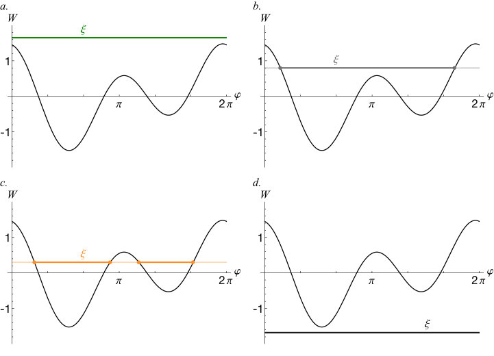 Figure 1
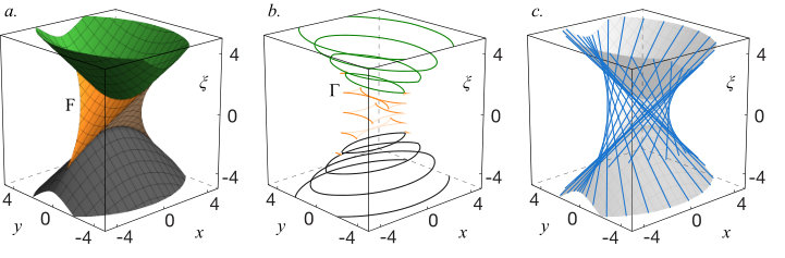 Figure 10
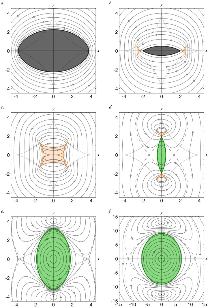 Figure 11
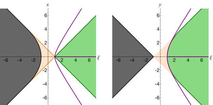 Figure 12
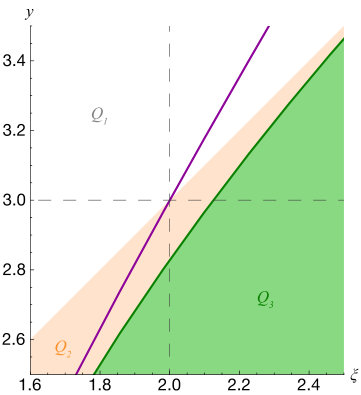 Figure 13
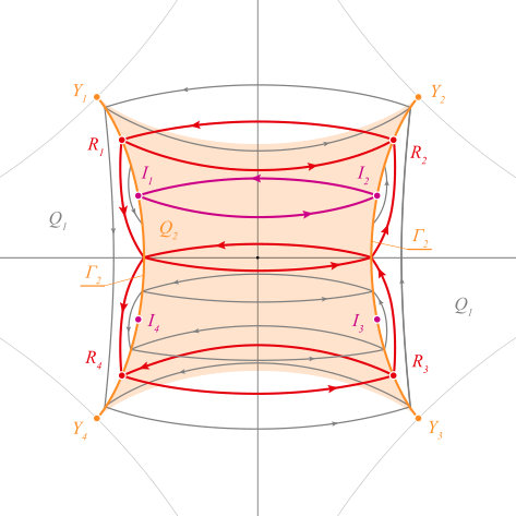 Figure 14
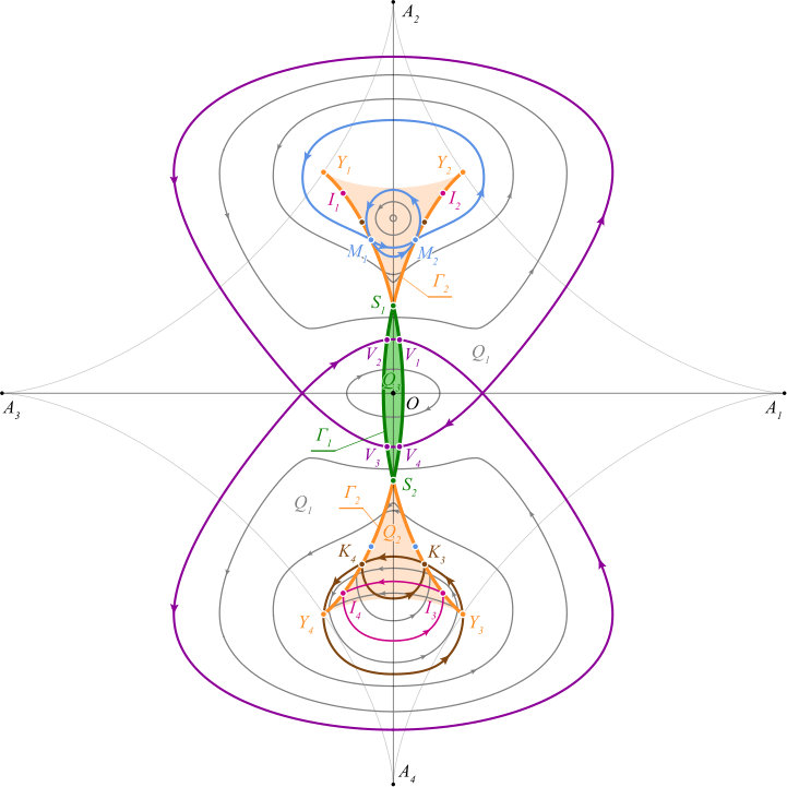 Figure 15
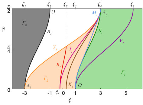 Figure 16
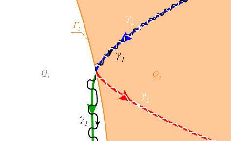 Figure 17
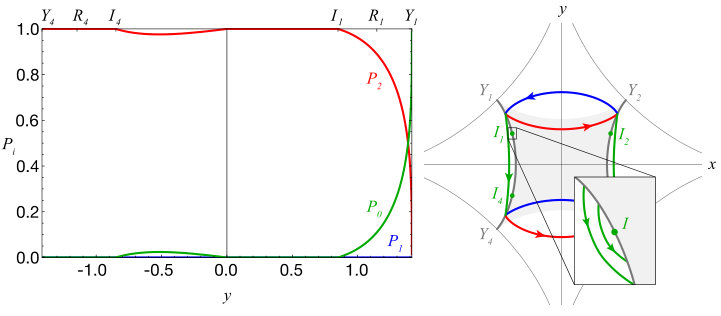 Figure 18
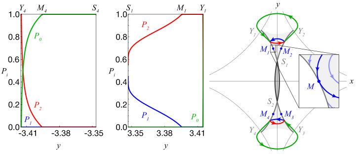 Figure 19
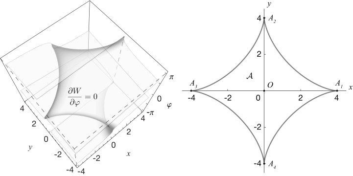 Figure 2
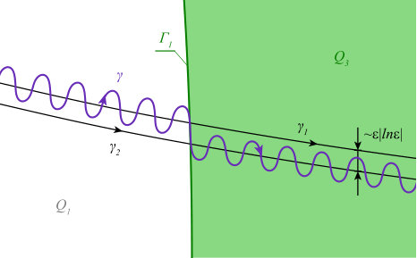 Figure 20
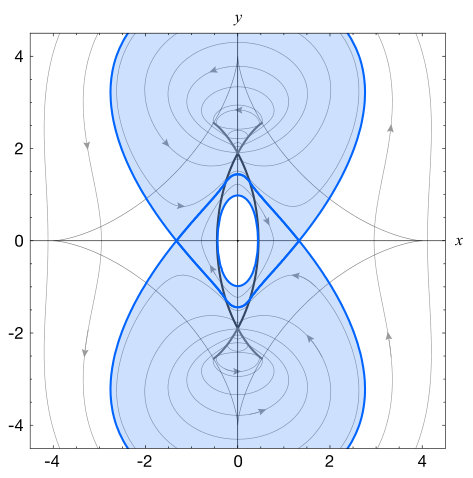 Figure 21
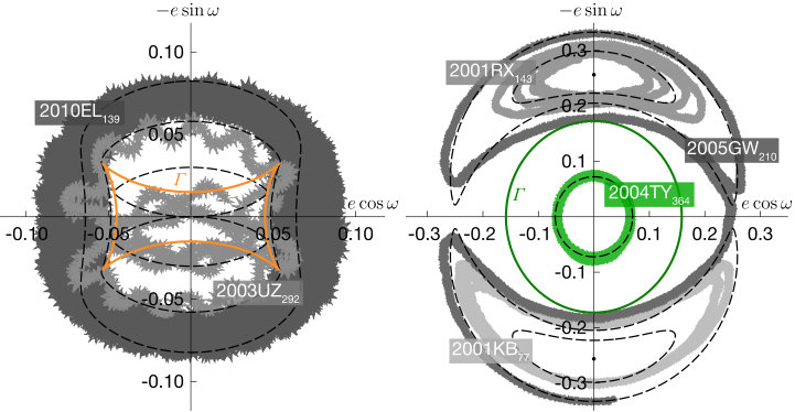 Figure 22
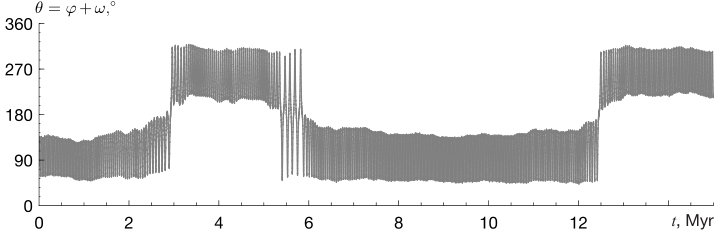 Figure 23
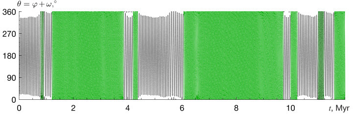 Figure 24
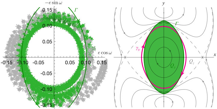 Figure 25
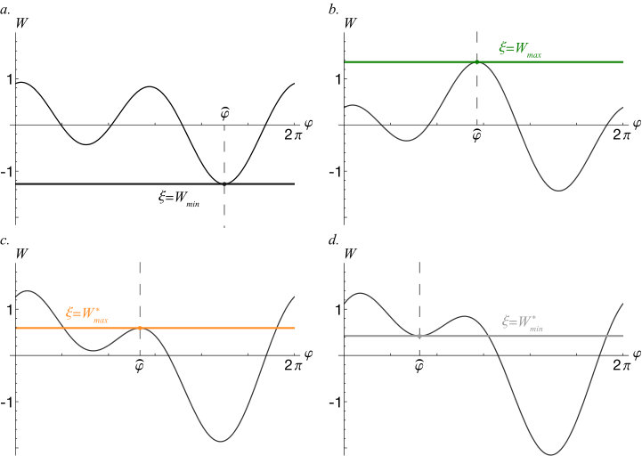 Figure 3
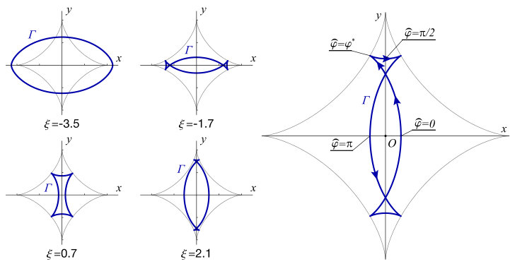 Figure 4
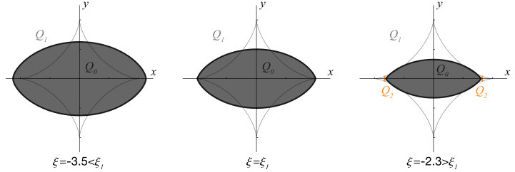 Figure 5
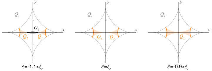 Figure 6
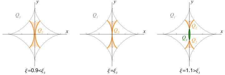 Figure 7
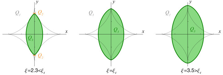 Figure 8
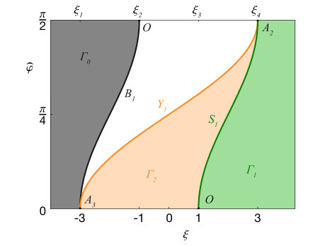 Figure 9
Peer Reviews
No public reviews on file for this paper yet. If you reviewed it on a platform where reviews are public (OpenReview, ICLR, NeurIPS, ICML), you can paste yours below so the community can read it here.
Videos
No videos yet. Explain this paper in a talk, walkthrough, or lecture? Add one.
Taxonomy
TopicsAstro and Planetary Science · Quantum chaos and dynamical systems · Stellar, planetary, and galactic studies
\journalname
Celestial Mechanics and Dynamical Astronomy
11institutetext: S. Efimov 22institutetext: Moscow Institute of Physics and Technology
9 Institutskiy per., Dolgoprudny, Moscow Region, 141701, Russian Federation
22email: [email protected] 33institutetext: V. Sidorenko 44institutetext: Keldysh Institute of Applied Mathematics
Russian Academy of Sciences,
Miusskaya Sq., 4, 125047 Moscow, Russian Federation
and
55institutetext: Moscow Institute of Physics and Technology
9 Institutskiy per., Dolgoprudny, Moscow Region, 141701, Russian Federation
Dynamics in first-order mean motion resonances: analytical study of a simple model with stochastic behaviour
S. Efimov
V. Sidorenko
Abstract
We examine a 2DOF Hamiltonian system, which arises in study of first-order mean motion resonance in spatial circular restricted three-body problem “star-planet-asteroid”, and point out some mechanisms of chaos generation. Phase variables of the considered system are subdivided into fast and slow ones: one of the fast variables can be interpreted as resonant angle, while the slow variables are parameters characterizing the shape and orientation of the asteroid’s orbit. Averaging over the fast motion is applied to obtain evolution equations which describe the long-term behavior of the slow variables. These equations allowed us to provide a comprehensive classification of the slow variables’ evolution paths. The bifurcation diagram showing changes in the topological structure of the phase portraits is constructed and bifurcation values of Hamiltonian are calculated. Finally, we study properties of the chaos emerging in the system.
keywords:
Hamiltonian system averaging method mean motion resonance chaotic dynamics
1 Introduction
The model system which will be considered below arises in studies of first-order mean motion resonances (MMR) in restricted three-body problem (R3BP) “star-planet-asteroid”. If asteroid makes revolutions around the star in the same amount of time in which the planet makes revolutions, there is an exterior resonance of the first-order denoted as . The term exterior refers to the fact that in this case the asteroid’s semi-major axis is larger than semi-major axis of the planet. The interior MMR takes place when asteroid makes revolutions during the time in which planet makes . The first-order MMRs are quite common and, therefore, intensively studied by many specialists. The related bibliography is given in Gallardo (2018) and Nesvorny et al. (2002). In particular, much effort has been spent to reveal why resonance with Jupiter corresponds to one of the largest gaps in the main asteroid belt (so-called Hecuba gaps), whereas MMR resonance is populated by numerous objects of Hilda group, and it is also very likely, that Thule group of objects in MMR is rather large (Broz and Vokrouhlicky, 2008; Henrard, 1996; Lemaitre and Henrard, 1990). The discoveries of trans-Neptunian objects made it urgent to study the exterior resonances with Neptune: twotino (MMR ) and plutino (MMR ) form big subpopulations in the Kuiper belt (Li et al., 2014a, b; Nesvorny and Roig, 2000, 2001).
It is possible to construct a model of dynamics in first-order MMR, taking into account only the leading terms in the Fourier series expansion of disturbing function (Sessin and Ferraz-Mello, 1984; Wisdom, 1986; Gerasimov and Mushailov, 1990). However, studies of planar R3BP (Beaugé, 1994; Jancart et al., 2002) revealed, that some important characteristics of first-order MMRs are reproduced only when the second-order Fourier terms are accounted for. In this paper we concentrate our attention on that part of a phase space, where eccentricities and inclinations are in relation (this, in some sense, is a case opposite to the planar problem, for which the relation is ). We intend to demonstrate, that in non-planar case second-order terms are no less important, as they make a model essentially stochastic. In contrast, the first-order models are proven to be integrable (Sessin and Ferraz-Mello, 1984), and thus cannot reproduce chaotic dynamics found in multiple numerical studies of first-order resonances (Wisdom and Sussman, 1988; Giffen, 1973; Winter and Murray, 1997a, b; Wisdom, 1987),
There are different mechanisms for generating chaos in the dynamics of celestial bodies (Holmes, 1990; Lissauer, 1999; Morbidelli, 2002). Presence of MMR may lead to the so-called adiabatic chaos (Wisdom, 1985), which is caused, roughly speaking, by small quasi-random jumps between regular phase trajectories in certain parts of the phase space, where adiabatic approximation is violated. Applying systematically Wisdom’s ideas to study of MMRs (Sidorenko, 2006; Sidorenko et al., 2014; Sidorenko, 2018), we found that adiabatic chaos often coexists with the quasi-probabilistic transitions between specific phase regions. Both phenomena occur in that part of the phase space, where the “pendulum” or first-order Second Fundamental Model for Resonance (Henrard and Lamaitre, 1983) approximations fail, because the first harmonic in the disturbing function Fourier series is not dominant. The goal of this paper is to carry out a comprehensive analysis of the introduced second-order model and investigate described mechanisms of chaotization, which, in our opinion, have not received proper attention in the past.
The paper is organized as follows. In Section 2 the model Hamiltonian system, which has a structure of slow-fast system, is introduced. In Section 3 the fast subsystem is studied. Equations of motion for slow subsystem are constructed in Section 4 and their solutions are analyzed in Section 5. Section 6 is devoted to different chaotic effects present in the discussed model. In Section 7 numerical evidence for existence of described phenomena is shown. The results are summarized in the last section. In Appendix A we reveal how the proposed model was derived. Details of the averaging procedure are elucidated in Appendix B.
2 Model Hamiltonian system
We are dealing with 2DOF Hamiltonian systems with specific symplectic structure:
[TABLE]
The Hamiltonian in (1) is expressed by
[TABLE]
Appendix A describes in detail how the system (1)-(2) arises in studies of first-order MMR in three-dimensional R3BP. Here we only note that
[TABLE]
where is the fraction of the planet’s mass in the total mass of the system, and denote the eccentricity and the argument of pericenter of asteroid’s osculating orbit respectively. Further is treated as a small parameter of the problem. Since in general variables vary with different rates (, while ), we can distinguish in (1) fast subsystem (described by the first line of equations) and slow subsystem (the second line).
In limiting case equations of fast subsystem coincide with equations of motion for particle with unit mass in a field with potential , where and are treated as parameters. Let
[TABLE]
be a solution of fast subsystem with fixed values of , , and value of Hamiltonian , which is the first integral of system (1). In general the resonant angle in (3) can librate between two constant values or change monotonously through the whole interval , i.e. circulate. In either case
[TABLE]
where is a period of the solution (3).
Because fast variables vary much faster then the slow ones, the right-hand sides in differential equations of slow subsystem in (1) can be replaced by their average values along the solution (3). This yields the evolution equations, which describe secular variations of and in closed form:
[TABLE]
Here
[TABLE]
The solution (3) has an action integral:
[TABLE]
For function becomes an adiabatic invariant of slow-fast system (1). For a fixed trajectories of averaged equations (4) on a phase plane go along the lines with constant values of . This allows to classify evolution equations (4) as adiabatic approximation (Neishtadt, 1987a; Wisdom, 1985).
In the next Sections we go through all the steps in construction of evolution equations via described approach and analyze in detail the behaviour of slow variables on different levels of Hamiltonian .
3 Properties of fast subsystem’s solutions for different values of slow variables (limiting case )
3.1 Partition of the plane based on the number of librating solutions
Because the variables and change very slowly (1), they can be treated as constant parameters, when considering the motion of the fast subsystem. Then the potential is just a “two-harmonic” function of defined on circle , and the motion in such potential can be described in terms of elliptic functions.
There are different types of motion depending on the Hamiltonian level at which it occurs (Fig. 1). For us it is important, that for some values of and two different librating solutions can exist on the same level (Fig. 1c). This situation can take place when has four extrema on .
A necessary condition for extremum after the replacement yields
[TABLE]
Let denote a region on the plane , in which has four extrema. The equation (7) has four real roots inside this region and only two outside. Thus on the border of the region the number of unique real roots is (with the exception of finite number of points in which there is only one unique real root) and the discriminant of (7) is equal to zero. Therefore the equation for the border of the region is
[TABLE]
By collecting the parts of this equation into perfect cube (8) is transformed to canonical algebraic equation of astroid (Fig. 2):
[TABLE]
Which can be further reduced to
[TABLE]
It is convenient to use this astroid for the reference on the phase plane .
3.2 Critical curve partitioning the plane into regions with different types of fast subsystem’ motion
Let us introduce the notations and for global minimum and maximum of function on for given values of slow variables. If , then has the second pair of minimum and maximum, which we shall denote and respectively. Using these auxiliary functions, we can partition the plane for a given into different regions based on the type of fast subsystem’s motion:
[TABLE]
The region will be called a forbidden region, because inside of it for any values of fast variables and fast subsystem has no solutions (Fig. 1d). Region is the region with the single librating solution (Fig. 1b), is the region with two librating solutions at given level (Fig. 1c), and finally the region is where fast subsystem’s solution circulates (Fig. 1a). Illustrations for regions will follow.
Before that let us consider a border between these regions. In every point of the border value of is equal to in one of its critical points (cf. Figures 1 and 3), which is why we shall call a critical curve. After replacement the equation transforms into algebraic equation:
[TABLE]
As Figure 3 demonstrates, the point lies on the critical curve when equation (11) have at least one multiple real root, which is equivalent to discriminant of (11) being equal to zero:
[TABLE]
Thus in the regions , , the discriminant , while in , and on the critical curve . Figure 4 depicts on the plane of slow variables for different values of . At critical curve have cusps, which lie on astroid (10). Additionally this curve may have points of self-intersection. If , the curve intersects itself on axis , with the coordinates of self-intersection points being defined by equation
[TABLE]
If , points of self-intersection lie on axis, and their coordinates are defined by equation
[TABLE]
The critical curve allows a parametrization
[TABLE]
which is illustrated by Figure 4. The parameter \mathord{\buildrel{\lower 3.0pt\hbox{\scriptscriptstyle\frown}}\over{\varphi}} in (13) coincide with the critical points of potential at given level , as depicted in Figure 3, in respective points of plane:
[TABLE]
The introduced parametric representation is convenient, in particular, for defining the location of cusps and self-intersection points. For cusps \mathord{\buildrel{\lower 3.0pt\hbox{\scriptscriptstyle\frown}}\over{\varphi}}={\varphi^{*}}, where is obtained from the equation , which have four roots on . We shall denote these cusps as ,…, with the lower index being the number of a quadrant, in which the respective value lies. Self-intersection points of on axis () we shall denote as and for right and left half-planes respectively. Self-intersection points on axis () we shall denote as and for upper and lower half-planes.
Note: It can be demonstrated, that curves are the involutes of astroid (10) constructed with tethers of length extended from astroid’s cusps. This makes also a family of equidistant curves with the distance between any two curves and .
3.3 Transformation of regions with change of
It should be noted first, that region with a single librating solution is present on plane for all values of . Other regions appear and disappear, as crosses several bifurcation values :
[TABLE]
We shall describe, how the regions are transformed, as increases.
If , there exists a forbidden region around the point , with the rest of plane being the region.
At on the right and on the left from region two parts of region (region with two librating solutions) appear (Fig. 5).
At the region disappears and becomes connected (Fig. 6).
At region is separated into two parts again by appearing region (region with circulating resonant angle) around the point as seen in Figure 7.
At region disappears (Fig. 8). For there exists only region surrounded by .
Let us now describe how borders of regions transforms with increase of . The border between and we shall call the existence curve and denote it as . It corresponds to the part of the critical curve in which . For curve . For curve consists of two intervals of , lying between points of self-intersection and .
We shall adopt the traditional terminology common in studies of slow-fast systems (Wisdom, 1985; Neishtadt, 1987a) with modifications made to better represent the specifics of the discussed problem. The border between regions and we shall call an uncertainty curve of the first kind and use a notation for it. Points of the uncertainty curve of the first kind are defined by condition . If , then . For , the curve consists of parts, which are contained between points of self-intersection and .
The part of the border between and , along which holds the equality , we shall call an uncertainty curve of the second kind and denote it . For the , where and are segments of , which lie between corresponding cusps. If then curve . For the rest part of the border between and holds . As no dynamical effects of interest are happening on this segment, we shall not refer to it further.
Figure 9 depicts a diagram, that shows values of \mathord{\buildrel{\lower 3.0pt\hbox{\scriptscriptstyle\frown}}\over{\varphi}} defining positions of cusps and self-intersection points on , as well as the segments which correspond to existence curve and two uncertainty curves. Due to the symmetry, it is sufficient to consider only \mathord{\buildrel{\lower 3.0pt\hbox{\scriptscriptstyle\frown}}\over{\varphi}}\in\left[0,\pi/2\right] (Fig. 4).
3.4 Three-dimensional representation of the set of curves
Curves can be interpreted as cross sections of some surface in the space by equi-Hamiltonian planes (Fig. 10a,b). In this space for fixed value of \mathord{\buildrel{\lower 3.0pt\hbox{\scriptscriptstyle\frown}}\over{\varphi}} the equations (13) define a straight line, which means that the surface is ruled (Fig. 10c).
The same surface defined by the equation analogous to (12) also appears in a completely different problem studied by Batkhin (2012), where it partitions the parametric space of some mechanical system into regions with different stability properties.
4 Evolution equations construction
4.1 Averaging along fast subsystem’s solutions
Considering that
[TABLE]
construction of the evolution equations (4) require calculating two averaged properties:
[TABLE]
The equality
[TABLE]
allows finding a period of fast subsystem’s solution at Hamiltonian level and calculating (after proper change of variables) values of integrals on the right-hand side of (14), e.g. for librating solutions:
[TABLE]
Here and denote minimum and maximum values of angle in librating solution, along which the averaging is being performed.
For the system (2) period and integrals (14) can be expressed in terms of complete elliptical integrals of the first and the third kind. Further the concise description of this transformation is given, using the case
[TABLE]
as an example. After standard substitution we obtain
[TABLE]
Here , . Function in (17) is a quartic polynomial
[TABLE]
with coefficients
[TABLE]
Integrals on the right-hand side in (17) can be rewritten as follows:
[TABLE]
where notation is used for integrals:
[TABLE]
– roots of polinomial , and the sign in the square root is determined by sign of coefficient . Integrals (19) can be presented as linear combinations of elliptic integrals of the first and the third kind:
[TABLE]
Analytical expressions for coefficients , , moduli , and parameters in (20) depend on integration interval and properties of roots. These expressions are gathered in the Appendix B.
Expressions of the kind
[TABLE]
can be further reduced to linear combinations of complete elliptic integrals of the first kind and the third kind with real parameter (Byrd and Friedman, 1954; Lang and Stevens, 1960). This, however, results in more complicated expressions, which is why we use representation (20).
When averaging along librating solutions of fast subsystem, which violate the condition (16), after substitution the integration in (17) is carried over two semi-infinite intervals. E.g., for the expression for the period is
[TABLE]
In these cases it is implied that all in (18) are the sum of two integrals as well.
After all described transformations evolution equations (4) take a simple form
[TABLE]
It should be noted, that there is an ambiguity in calculation of the right-hand side parts of evolution equations in the region : the result depends on the choice of the fast subsystem’s solution, and there are two different librating solutions in . Consequently, phase portraits of (4) shall contain two sets of trajectories in , which correspond to two possible variants of slow variables’ evolution.
When describing the crossing of uncertainty curves by the projection of the phase point on the plane , we shall confine ourselves to formal continuation of averaged system’s trajectories, lying on opposite sides of . The detailed analysis of these events is given in Neishtadt (1987a), Neishtadt and Sidorenko (2004), and Sidorenko et al. (2014).
4.2 Fast subsystem’s action variable – integral of evolution equations
As was mentioned in the Section 2, adiabatic invariant of slow-fast system is a first integral of evolution equations (4). Formula (6) for can be expressed as a linear combination of integrals defined by (19):
[TABLE]
Analytical expression for is presented in the Appendix B alongside the rest of the integrals previously shown in (20).
5 Study of slow variables’ behavior using evolution equations
5.1 Phase portraits of evolution equations. Stationary points
To analyze solutions of the slow subsystem (4), we build its phase portraits. For values the structure of phase portrait is simple – all phase trajectories are represented by closed loops encircling the forbidden region (Fig. 11a). Figure 11b depicts a typical phase portrait for – two symmetrical parts of region adjoining the central region contain two layers of phase trajectories. For there are only two regions on the phase plane, i.e. and (Fig. 11c). In addition to presented in Figure 11c,d change of phase portrait’s global structure, the behaviour of phase trajectories near the uncertainty curves at have some specific qualitative differences at different values. The detailed description of that is given in the end of this section.
Phase portraits at have five stationary points: the origin of -plane is the stable point of the center type, two more center points are symmetrically located on the -axis, and two unstable saddle points are symmetrically located on the -axis (Fig. 11d–f). Phase portraits depicted in Figures 11e and 11f are differ in relative positions of heteroclinic trajectories and uncertainty curve .
Ordinates of the center points above and below plane’s origin are defined by equation
[TABLE]
where
[TABLE]
Abscissae of the saddle points are defined by the same relation (23) with different parameters:
[TABLE]
Solutions of (23) are plotted in Figure 12 as functions of for both types of stationary points. Note, that top and bottom center points are located in at and in at (Fig. 13).
5.2 Limiting points on uncertainty curves
To conclude the description of how phase portraits’ topology changes with value, points of uncertainty curves’ intersections with limiting trajectories, that are limiting cases for different families of trajectories, should be considered. We shall refer to them as limiting points.
Several types of limiting points are depicted in Figure 14. Trajectories, which go in between two points on uncertainty curve , can be divided into two families: the trajectories that intersect axis, and those that do not. Thus there is limiting trajectory that separates these two families (in Figure 14 it is colored red). We shall denote the limiting points corresponding to this trajectory as (Fig. 14). The subset of trajectories, which do not cross -axis in as another limiting case contain trajectories, which come to uncertainty curve from the side of and then reflect back without exiting to . In Figure 14 these trajectories are colored purple, and the corresponding limiting points are denoted .
More limiting points are depicted in figure 15. Points are connected to cusps by limiting phase trajectories, which separate the family of trajectories lying to the one side of uncertainty curve from those which in connect symmetric points on left and right sides of uncertainty curves . Limiting points divides each of four segments (located in each of four quadrants of plane) into two sections: one section has both trajectories, which adjoin from side, going in the same direction, while trajectories adjoining the other section go in opposite directions (also see Figure 19). Points of curve’s intersections with mentioned earlier separatrices constitute the last type of limiting points.
All differences between the phase portraits (Fig. 11) emerge from changes in position of limiting points on the critical curve. By adding these points to diagram in Figure 9 we obtain a bifurcation diagram (Fig. 16), from which all changes in topological structure of phase portraits can be understood. Let us describe, what is happening to different limiting points by going successively from low to high values of . The first limiting points – and – appear at . At points merge with cusps , and at the same time points appear. Points and emerge simultaneously with region and self-intersections points of the critical curve at . All points on the part of the critical curve – , , and , as well as the ends , of itself – disappear at merging with the astroid’s cusps and . Finally, at points disappear by merging pairwise.
Bifurcation Hamiltonian values partition the whole range of into nine intervals, meaning that there is a total number of nine different types of phase portraits for slow subsystem. The bifurcation at (Fig. 13) is omitted from Figure 16 because it does not bear any significance for the dynamical effects considered further.
6 Quasi-random effects
6.1 Probabilistic change of fast subsystem’s motion regime on the uncertainty curve of the second kind
In each point of three guiding trajectories, i.e. trajectories of averaged system (4), meet: two on the side of region and one on the side. In the case, when two out of these three trajectories are outgoing, the transition of the phase point to either one of them can be considered as a probabilistic event. In the original system (1) initial values of fast variables corresponding to two different outcomes are strongly mixed in the phase space. Therefore even small variation of initial conditions can lead to qualitative change in system’s evolution. As an example, Figure 17 depicts projections on the plane of two trajectories , obtained as solutions of the system (1) with close initial conditions. Both trajectories approach uncertainty curve along the same guiding trajectory, but diverge after that – exits and follows the outgoing guiding trajectory in , while turns and goes back along the other guiding trajectory in .
In deterministic systems with strongly entangled trajectories the probability of a specific outcome is determined by the fraction of phase volume occupied by corresponding initial conditions (formal definition can be found in Arnold (1963) and Neishtadt (1987b)). In order to find the probabilities of transitions to different outgoing trajectories in some point on , two auxiliary parameters must be calculated first (Neishtadt, 1987b; Artemyev et al., 2013):
[TABLE]
These parameters have a meaning of rates with which areas bounded by separatrices and in fast variables’ phase space change. After substitution of specific potential function (2) into (24) and change of integration variable to we obtain:
[TABLE]
Here \mathord{\buildrel{\lower 3.0pt\hbox{\scriptscriptstyle\frown}}\over{\varphi}} is the coordinate of the saddle point in the fast subsystem’s phase portrait (it coincides with the value \mathord{\buildrel{\lower 3.0pt\hbox{\scriptscriptstyle\frown}}\over{\varphi}} corresponding to point in (13)); and are the minimal and the maximal values of in homoclinic trajectories to the left and to the right of the saddle point respectively. Applying the substitution \lambda=\cot[{{(\varphi-\mathord{\buildrel{\lower 3.0pt\hbox{\scriptscriptstyle\frown}}\over{\varphi}})}/2}] to (25) we obtain:
[TABLE]
where
[TABLE]
[TABLE]
It should be noted, that inequalities and hold for all points of . Integration in (26) is carried out over the intervals and for and respectively. The result can be obtained by using Cauchy’s residue theorem:
[TABLE]
Here
[TABLE]
and the branches of multifunctions are selected in such way, that , , and .
Now we can write down the expressions for probabilities of different evolution scenarios for a phase point on . Let us denote the probability of point going to region as , and probabilities corresponding to two trajectories going inside as and . The resulting formulae (Artemyev et al., 2013) take a form:
[TABLE]
where
[TABLE]
In Figure 18 and Figure 19 change of probabilities (27) along is shown alongside with phase portraits at corresponding values of Hamiltonian and limiting points, which mark the change of sign in or .
6.2 Adiabatic chaos
Adiabatic chaos emerges due to non-applicability of adiabatic approximation near the uncertainty curve. As a result the projection of phase point leaves the vicinity of uncertainty curve along the guiding trajectory, which slightly differs from the direct continuation of approach trajectory (Fig. 20). The resulting offset between incoming and outgoing guiding trajectories can be treated as a quasi-random jump with order of magnitude (Tennyson et al., 1986; Neishtadt, 1987b, a).
As a result of persistent jumps any trajectory that crosses the uncertainty curve after a long time will fill a whole region of phase plane, which we will call an adiabatic chaos region (Fig. 21). This region consists of points belonging to trajectories, which cross the uncertainty curve.
At the uncertainty curve is crossed by the separatrices, which connect two saddle points. A phase point projection moving along a guiding trajectory close to separatrix, when crossing the uncertainty curve, may jump over the separatrix and begin to move along the other guiding trajectory belonging to completely different family. Thus the properties of long-term evolution are suddenly changed on a qualitative level. E.g., in Figure 21 the motion of a phase point projection circling around the coordinate origin in the central part of adiabatic chaos region by crossing the separatrix may transform into circulation in opposite direction around one of two center points (23), which lie on -axis in upper or lower half-plane. This event can be interpreted as a capture into Kozai-Lidov resonance and it is accompanied by decrease of average inclination value, about which the long-term oscillations occur.
7 Numerical simulations
Construction of the discussed analytical model involved several assumptions that may seem loose. It is thus required to test whether the model can be applied to orbital dynamics of real life objects and these assumptions were not overly restrictive.
For this purpose we used Mercury integrator (Chambers, 1999) and carried out several numerical simulations of the Solar system composed of the Sun, the four giant planets, and about 700 known Kuiper belt objects (KBO) near , , and resonances with Neptune represented by test particles (masses of four inner planets were added to the Sun in order to facilitate the integration). Total time of integration is one order of magnitude larger then the characteristic time of slow variables evolution (given the orbital period of Neptune and Neptune/Sun mass ratio defining the small parameter ).
For interpretation of the simulation results we shall utilize a scaled version of previously used slow variables:
[TABLE]
For exact relations between and , as well as the expression for small parameter , see Appendix A.
Phase trajectories of several objects are plotted in Figure 22. Main sources of difference between analytical phase portraits and numerical ones are non-zero eccentricity of Neptune (), high eccentricity of KBOs (up to on the right side of Figure 22), and presence of other planets, which introduce additional disturbances distorting the phase plane. Nevertheless, it is clear that the overall topological structure of phase portraits is reproduced in analytical model. Note, that in restricted three-body problem all solutions of Sessin and Ferraz-Mello (1984) on the same phase plane would be represented by concentric circles with and changing linearly with time.
The principal difference between our model and the one introduced by Sessin and Ferraz-Mello (1984) is the expansion of disturbing function past the first term in the Fourier series. Thus we can assert, that the region of the complete phase space, where the second term influences the dynamics in a substantial way, is significantly large. Indeed about of objects in our simulations deviated from circular trajectories in projection on the plane of slow variables. The rest correspond to very high or very low values of , at which all trajectories in and , as well as the curve separating them, in our model are likewise very close to circles.
Some effects, that can be derived from the analytical model, are also observed in numerical simulations within the pool of selected KBOs. E.g. resonant angle of shows jumps between two different librating regimes characteristic to motion in region (Fig. 23), while demonstrates the intermittent behaviour (Fig. 24) with the resonance angle constantly switching between libration and circulation. Phase trajectory of on the plane of slow variables is presented in Figure 25, showing that changes in resonant angle behaviour are conditioned by secular trajectory crossing of the critical curve . Similarly, analytical trajectory goes between regions of libration and circulation of resonant angle (Fig. 25). To compensate for angle precession on this kind of trajectories the modified resonant angle was used in previous plots111The resonant angle is the “standard” one for studies of first-order MMR (Murray and Dermott, 2000). Our choice of the resonant angle was determined by the desire to write down the Hamiltonian of the system in the form (2), which seem to us most convenient for the analysis.. Same as , resonant angle circulates in and librates in and .
8 Conclusion
In this paper, using the averaging technique, we study Hamiltonian system that approximately describes the dynamics of a three-body system in first-order MMR (within the restricted circular problem). Our model incorporates harmonics of the Fourier series expansion of disturbing function up to the second order. Thus it can accurately describe the dynamics in that part of the phase space where first two harmonics have comparable magnitudes, and where the well known integrable model of first-order MMR is not applicable. This is the region, from which chaos emerges.
The nonintegrability of our model does not become an obstacle for a detailed analytical investigation of its properties. In particular, we have constructed bifurcation diagrams and phase portraits characterizing the long-term dynamics on different level sets defined by the system’s Hamiltonian and obtained expressions for probabilities of quasi-random transitions between different phase trajectories.
The important question is the scope of the correctness of proposed model. We will try to answer it in subsequent studies, using Wisdom’s approach to investigate several first-order MMRs without truncating the averaged disturbing function. Nevertheless, even now we can note that the secular evolution of some Kuiper belt objects qualitatively resembles what our simple model predicts.
We hope also that our investigation outlines an approach which can be applied for analysis of similar degeneracy of the averaged disturbing function in the case of other MMRs (e.g., Sidorenko (2006)).
Appendix A: Constructing a model system, that reveals the origin of chaos in first-order MMR
We shall confine ourselves to a case of exterior resonance in restricted three-body problem. The interior resonance can be reduced to the same model using similar approach. The distance between the two major bodies, i.e. a star and a planet, and the sum of their masses are taken here as units of length and mass. The unit of time is chosen such that the orbital period of major bodies’ rotation about barycenter is equal to . The mass of the planet is considered to be a small parameter of the problem.
Equations of motion for minor body (asteroid) in canonical form:
[TABLE]
where are the Delaunay variables (Murray and Dermott, 2000). They can be expressed in terms of Keplerian elements as
[TABLE]
The last variable is the asteroid’s mean anomaly.
Hamiltonian in (28) is
[TABLE]
Here is disturbing function in restricted circular three-body problem. Mean anomaly appearing in (29) depends linearly on time: . Therefore it is convenient to use variable instead of , as it enables writing down the equations of motion in autonomous form as canonical equations with Hamiltonian
[TABLE]
We introduce resonant angle using the canonical transformation defined by generating function
[TABLE]
where , while is the value of corresponding to exact MMR in unperturbed problem (). The new variables are related to the old ones as follows:
[TABLE]
The resonant angle can also be expressed in traditional form
[TABLE]
New Hamiltonian
[TABLE]
The resonant case we are interested in corresponds to region of phase space, selected by the condition
[TABLE]
Here and are mean motions of planet and asteroid respectively. It is also true in that
[TABLE]
In the resonant case, i.e. when the previous inequation holds, variables can be divided into fast, semi-fast and slow. Fast and semi-fast variables in are and respectively:
[TABLE]
Slow variables, which vary with a rate of order , are , , , and .
To study secular effects the averaging over the fast variable is performed, which results in equations of motion taking a canonical form with Hamiltonian
[TABLE]
where
[TABLE]
After such averaging the fast variable vanishes, and the term “fast” is exempted. Thus in the rest of the paper we adopt name fast for denoting variables, which vary with the rate , instead of referring to them as semi-fast, when the distinction of three different time scales was needed.
Moreover, because there is no longer in the Hamiltonian , the conjugate momentum is a constant in considered approximation and can be treated as a parameter of the problem. Thus is the Hamiltonian of a system with two degrees of freedom. Further instead of we shall use parameter
[TABLE]
Inequation defines region in phase space, to which the motion of the system is bound by the Kozai-Lidov integral (Sidorenko et al., 2014).
Next standard step in analysis of system’s dynamics in resonant region is the scaling transformation (Arnold et al., 2006):
[TABLE]
where is a new small parameter. Using variables (31), the equations of motion can be rewritten in a form of slow-fast system without loss of accuracy:
[TABLE]
Here
[TABLE]
For the approximate expression for can be obtained as a series expansion (Murray and Dermott, 2000):
[TABLE]
where
[TABLE]
Expressions (34) are obtained taking into account resonance condition (30), and that the values and are limited by , leading to .
Coefficients , , , , , in (33) are calculated as follows:
[TABLE]
Here , is the Kronecker delta, and , are Laplace coefficients. Numerical values of coefficients (35) for several resonances are gathered in Table 1.
Out of the whole region we are interested in the part with small eccentricities. Thus we further assume , which leads to . Taking into account (34) we can write down expression for averaged disturbing function up to the terms of order :
[TABLE]
By introducing the variables
[TABLE]
the equations of motion (32) can be reduced to a Hamiltonian form
[TABLE]
with the Hamiltonian
[TABLE]
The final rescaling of variables
[TABLE]
results in the model system (1)–(2).
Appendix B: Analytical expressions for integrals, emerging during the averaging over fast subsystem’s period
Right-hand side parts of evolution equations (4), as well as adiabatic invariant formula (22), can be expressed in terms of integrals
[TABLE]
where ; , and integration limits , can be either real numbers or . These integrals can be reduced to the linear combinations of elliptic integrals of the first, the second and the third kind:
[TABLE]
Further the formulae for coefficients , , moduli and parameters are gathered for all necessary cases.
The case
We will further assume, that are numbered in ascending order:
[TABLE]
Four different instances should be considered:
- A.
Integration over ; 2. B.
Integration over ; 3. C.
Integration over ; 4. D.
Integration over .
Instance A
Here and . We shall also use the following auxiliary parameters:
[TABLE]
The value of elliptic integrals’ modulus in (37):
[TABLE]
and parameter .
In order to find coefficients in (37), we considered such linear combinations of , that are reduced to integral (253.39) from (Byrd and Friedman, 1954):
[TABLE]
After some simple calculations, one can find:
[TABLE]
Using (253.00) from Byrd and Friedman (1954) we also obtain:
[TABLE]
Instance B
For integrals over the interval the only difference is the parameters , and modulus . Thus in (39) the values
[TABLE]
should be used.
Instance C
For integrals over the interval in (39):
[TABLE]
The modulus and parameter are the same as for interval .
Note: The equality of and in instances and means, that when the potential (2) has two minima, the periods of librations about them on the same energy level are equal. This also holds true for local minima corresponding to instances and , as the substitution always allows to get rid of semi-infinite intervals of integration. Moreover, the averaged values of in (18) are also the same for librations around two local minima. The averaged values of in (18) for librations about two local minima differ by , and values of adiabatic invariant (22) differ by .
Instance D
For integrals over two semi-infinite intervals the values of parameters in (39) are
[TABLE]
The modulus is the same as for integration over , and is the same as for .
The case (), ()
Here there are only two instances:
- A.
Integration over ; 2. B.
Integration over .
Instance A
Here the following auxiliary parameters in expressions for and will be used:
[TABLE]
[TABLE]
where
[TABLE]
Using (38) and formulae (259.04), (341.01)–(341.04)222It should be noted, that (259.04) in (Byrd and Friedman, 1954) contain a typo – the multiplier (in authors’ notation) is missing. from (Byrd and Friedman, 1954), we obtain
[TABLE]
Modulus and parameter of elliptic integrals are calculated as follows:
[TABLE]
Instance B
Expressions (41) stay the same. Auxiliary parameters are
[TABLE]
[TABLE]
The modulus of elliptic integrals is also different:
[TABLE]
The case
Let us denote real parts of roots as , and imaginary parts as :
[TABLE]
Without loss of generality let us assume, that , , and (if , then also ). In expressions for and the following auxiliary parameters will be used
[TABLE]
[TABLE]
Similar to previous case we find:
[TABLE]
Modulus and parameter of elliptic integrals:
[TABLE]
Acknowledgements.
The work was supported by the Presidium of the Russian Academy of Sciences (Program 28 “Space: investigations of the fundamental processes and their interrelationships”). We are grateful to A.I.Neishtadt, A.Correia, A.Morbidelli and J.Wisdom for useful discussions. We would also like to thank D.A.Pritykin for proofreading the manuscript.
The reference list from the paper itself. Each links out to its DOI / PubMed record.
- 1Arnold et al. (2006) Arnold V, Kozlov V, Neishtadt A (2006) Mathematical Aspects of Classical and Celestial Mechanics, 3rd edn. Springer, New York
- 2Arnold (1963) Arnold VI (1963) Small denominators and problems of stability of motion in classical and celestial mechanics. Russian Mathematical Surveys 18(6(114)):91–192
- 3Artemyev et al. (2013) Artemyev AV, Neishtadt AI, Zeleny LM (2013) Ion motion in the current sheet with sheared magnetic field – Part 1: Quasi-adiabatic theory. Nonlin Processes Geophys 20:163–178
- 4Batkhin (2012) Batkhin AB (2012) Application of the method of asymptotic solution to one multi-parameter problem. in: Gerdt V.P., Koepf W., Mayr E.W., Vorozhtsov E.V. (eds) Computer Algebra in Scientific Computing. CASC 2012. Springer, Berlin, Heidelberg, Lecture Notes in Computer Science, vol 7442, pp 22–33
- 5Beaugé (1994) Beaugé C (1994) Asymmetric liberations in exterior resonances. Celestial Mechanics and Dynamical Astronomy 60(2):225–248
- 6Broz and Vokrouhlicky (2008) Broz M, Vokrouhlicky D (2008) Asteroid families in the first-order resonance with Jupiter. MNRAS 390:715–732
- 7Byrd and Friedman (1954) Byrd PF, Friedman MD (1954) Handbook of elliptic integrals for engineers and physicists. Springer-Verlag, Berlin-Göttingen-Heidelberg
- 8Chambers (1999) Chambers JE (1999) A hybrid symplectic integrator that permits close encounters between massive bodies. Monthly Notices of the Royal Astronomical Society 304(4):793–799