Stability Within $T^2$-Symmetric Expanding Spacetimes
Beverly K. Berger, James Isenberg, Adam Layne

TL;DR
This paper extends the understanding of the stability and asymptotic behavior of $T^2$-symmetric Einstein solutions by proving a nonpolarised analogue with broader applicability, supported by numerical simulations.
Contribution
It introduces a nonpolarised analysis of $T^2$-symmetric Einstein flows, generalizing previous polarised results and revealing the instability of polarised asymptotics.
Findings
Similar decay rates for normalized energy in the broader class
Existence of a locally attractive set outside the main theorem's scope
Polarised asymptotics are shown to be unstable
Abstract
We prove a nonpolarised analogue of the asymptotic characterization of -symmetric Einstein Flow solutions completed recently by LeFloch and Smulevici. In this work, we impose a condition weaker than polarisation and so our result applies to a larger class. We obtain similar rates of decay for the normalized energy and associated quantities for this class. We describe numerical simulations which indicate that there is a locally attractive set for -symmetric solutions not covered by our main theorem. This local attractor is distinct from the local attractor in our main theorem, thereby indicating that the polarised asymptotics are unstable.
Click any figure to enlarge with its caption.
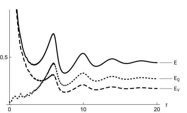 Figure 1
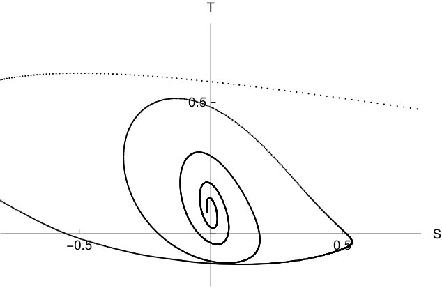 Figure 2
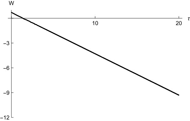 Figure 3
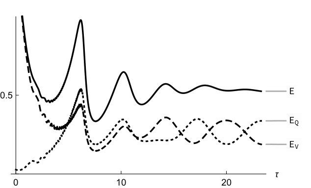 Figure 4
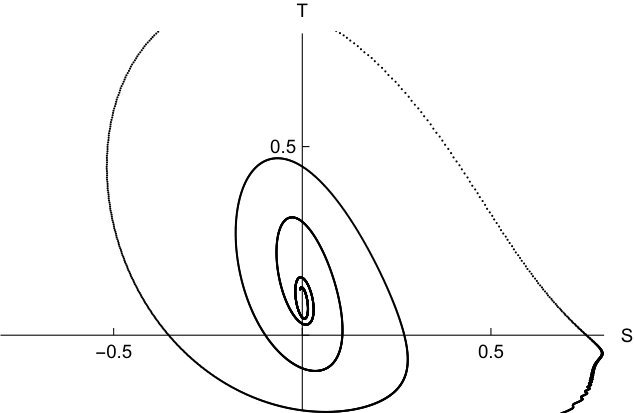 Figure 5
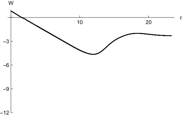 Figure 6
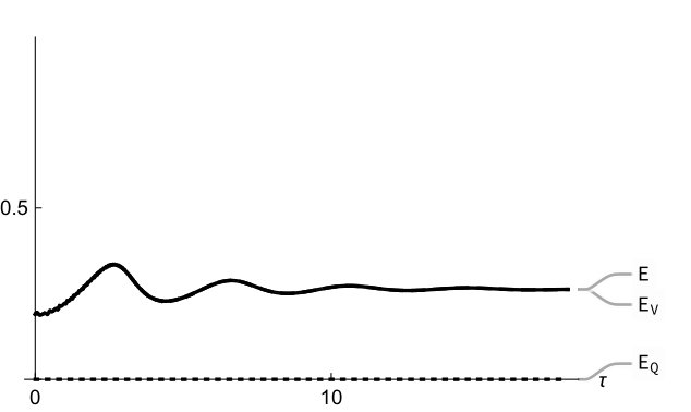 Figure 7
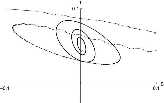 Figure 8
 Figure 9
Peer Reviews
No public reviews on file for this paper yet. If you reviewed it on a platform where reviews are public (OpenReview, ICLR, NeurIPS, ICML), you can paste yours below so the community can read it here.
Videos
No videos yet. Explain this paper in a talk, walkthrough, or lecture? Add one.
Stability Within -Symmetric Expanding Spacetimes
Beverly K. Berger
Edward L. Ginzton Laboratory
Stanford University
Stanford, CA 94305-4088
USA
,
James Isenberg
Department of Mathematics
University of Oregon
Eugene, OR 97403-1222
USA
and
Adam Layne
Department of Mathematics
KTH Royal Institute of Technology
100 44 Stockholm
Sweden
Abstract.
We prove a nonpolarised analogue of the asymptotic characterization of -symmetric Einstein Flow solutions completed recently by LeFloch and Smulevici. In this work, we impose a condition weaker than polarisation and so our result applies to a larger class. We obtain similar rates of decay for the normalized energy and associated quantities for this class. We describe numerical simulations which indicate that there is a locally attractive set for -symmetric solutions not covered by our main theorem. This local attractor is distinct from the local attractor in our main theorem, thereby indicating that the polarised asymptotics are unstable.
1. introduction
There exist broad conjectures about the expanding direction behavior of vacuum spacetimes with closed Cauchy surfaces [2, 9], but currently little is known about some of the most elementary examples. Recent results [13, 18] have demonstrated that certain vacuum cosmological models demonstrate locally stable behavior in the expanding direction, but that well-known subclasses are unstable. These results should be compared to models with matter [16, 23, 22, 21] where spatially homogeneous solutions are known to be stable. It is also important to note that the behavior of these models in the direction of the singularity is not sensitive to the presence of most types of matter [3].
In the special case that the spacetime has spatial topology , admits two spacelike Killing vector fields (such spacetimes are called -symmetric), and satisfies a further technical condition (that the spacetime is polarised) results of [13] show that there is a local attractor of the Einstein Flow in the expanding direction. It is natural to ask whether the condition that the spacetime be polarised is necessary. Do spacetimes on with two spacelike Killing vector fields necessarily become effectively polarised? Do they then flow to the polarised attractor?
We partially resolve these questions by analytic and numerical means. Our main theorem states that solutions which are not polarised have the expanding direction asymptotics of polarised solutions if they satisfy a certain weaker condition: that one of the two conserved quantities of the flow vanishes. We call such solutions or solutions. The conserved quantity vanishes for all polarised solutions; the set of solutions is of codimension one in the space of all solutions in these coordinates while the set of polarised solutions is of infinite codimension.
It was shown in [6] that -symmetric vacuum spacetimes posess a global foliation; all such Einstein Flows have a metric of the form
[TABLE]
where and are the Killing vector fields. The area of the orbit is , so the singularity occurs as and the spacetime expands as . Relative to the coordinates used in [18], our quantities are given by
[TABLE]
See the Appendix for a complete concordance of notations between the cited papers and the present work. In the coordinates (1.1), the Einstein Flow is
[TABLE]
The last equation is the momentum constraint, and it is preserved by the evolution equations. Equation (1.8) is a consequence of the constraints; satisfies a wave equation similar to (1.5) which can be derived as a consequence of (1.7) and (1.8), so we take equations (1.5) through (1.8) to be the evolution equations instead. There are, in addition, evolution equations for , but these may be integrated once have been found, so these latter four functions are the ones of interest. As a consequence of (1.5) and (1.6), there are two conserved quantities along the flow:
[TABLE]
The condition is often imposed when studying these solutions in the collapsing direction. Such solutions are called polarised. (Note that all polarised solutions have , but not all solutions are polarised.) The constant is, without loss of generality, that “twist constant” which cannot in general be made to vanish by a coordinate transformation. The Gowdy models [10] are those for which . -symmetric spacetimes which are polarised, half polarised [11, 8], or Gowdy have been studied extensively in the contracting direction (e.g. [1]). We are here concerned only with the expanding direction.
The Kasner models are those which are spatially homogeneous ( are independent of ) and satisfy . Let us note that, in our coordinates, polarised Kasner solutions [12] take the form
[TABLE]
for some constants . The Gowdy models contain all Kasners, and in the expanding direction the dynamics of Gowdy solutions are known [17], [19] and appear to be very different from those of non-Gowdy solutions. Non-Gowdy solutions such that are independent of are called pseudo-homogeneous or PH. This definition appears in [18], where it is shown that the future asymptotics are of the form
[TABLE]
That is, PH solutions have asymptotics of the same form as a Kasner solution, but the value of at is restricted.
In contrast to these examples, in [13] the authors find a set of non-Gowdy, polarised solutions such that
[TABLE]
The results in [18] and [13] are much more detailed than the above statements; we give this simple description only to demonstrate that an instability arises; no polarised Kasner or PH solutions can have future behavior of the form (1.14). The relationships between these sets of solutions are given in Figure 1.
Previous to this work, numerical simulations conducted by Berger [4, 5] indicated that all -symmetric solutions, without regard to the polarisation or smallness conditions imposed in [13], flowed toward the polarised attractor (1.14). In addition, in [18] it is shown that within the neighborhood of each polarised PH solution is a polarised non-PH solution with future asymptotics of the form (1.14).
Before giving a description of our main theorem, let us note the sense in which we use the word “attractor.” Our technique of proof follows [13]. Let us denote the right side of (1.7) by . The idea of the proof is to treat the asymptotic regime of the solution as a wave equation for coupled to an ordinary differential equation (up to some error terms) for the means in the -direction of . The smallness assumptions are then used to guarantee that the errors decay, and so the behavior of the means of approaches the behavior of the solution of the ODE. When we use the word “attractor” here, we refer to the dynamics of the system; a solution is not generally a proper attractor of the flow in the sense that
[TABLE]
in norm.
Our main theorem states roughly that the condition suffices to ensure that a solution has polarised asymptotics if it begins sufficiently close to the asymptotic regime. In the latter portion of the paper, we present numerical evidence that the condition is necessary for the solution to have polarised asymptotics and flow toward the polarised attractor. There appears to be an attractor for solutions satisfying , which shares some formal properties with the attractor. However, such solutions flow away from the attractor, and so the asymptotics appear to be unstable.
Since the future behavior of Gowdy and PH solutions is understood, we are only concerned with non-Gowdy, non-PH solutions; that is, solutions with and unbounded as . In this case, we shift by a constant
[TABLE]
so that
[TABLE]
In the rest of the paper, we assume solutions are non-Gowdy and so change variables to to avoid writing factors of .
Before proceeding with the proof, it is important to note that there is some very interesting work on the rescaling limits of certain expanding spacetimes [14, 15]. The earlier of these works uses techniques from the study of Ricci Flow to analyze the rescaling limits of CMC-foliated expanding spacetimes. The latter work is concerned with the extent to which rescaling limits of the spacetimes considered in [13] have a nonzero Einstein tensor. It is likely that this result can be generalized to the class of solutions considered in this paper.
Acknowledgements. We are grateful to David Maxwell, Peng Lu, Paul T Allen, Florian Beyer, Piotr Chruściel, Anna Sakovich, and Hans Ringström for providing useful comments on various parts of this project.
The second and third authors were supported by NSF grants DMS-1263431 and PHY-1306441. This article was in part written during a stay of the third author at the Erwin Schrödinger Institute in Vienna during the thematic program ‘Geometry and Relativity’. This paper incorporates material that previously appeared in the third author’s dissertation which was submitted to the Department of Mathematics in partial fulfillment of the requirements for the degree of Doctor of Philosophy at the University of Oregon.
2. Preliminary Computations
Before proceeding with the proof of the main theorem, we define the energy under consideration and calculate its evolution. It is useful to have notation for the mean of a function in the -direction.
Definition 2.1** (-mean).**
For , let
[TABLE]
Note that in [13], the authors choose to use the volume form for their mean. Our choice is almost identical to that used in [18], but we normalize so that . Either choice would suffice.
Define the following energy
[TABLE]
and the -volume
[TABLE]
Note that equation (1.7) now reads . We use the terms -energy and -energy loosely to refer to and , respectively. One may compute using the evolution equations for and that
[TABLE]
so the energy evolves by
[TABLE]
The terms appearing here are undesirable for proving energy inequalities. This necessitates the modification of by a term which trades for . This is the main topic of Section 3.
3. corrections and their bounds
Define the correction
[TABLE]
Corrections to the energy of essentially this form were used previously in the Gowdy case [17] and in the existing results on -symmetric spacetimes [18, 13]. Our definition differs only slightly from those previously used. Differentiating (3.1) and using integration by parts yields the two components of the -energy, but with opposite sign. This allows us to replace time derivatives by space derivatives, which may be bounded. At the same time, the correction has better decay properties than the energy, and so we are able to draw conclusions about the energy in the expanding direction.
To trade for and for , it would be more natural to consider the corrections
[TABLE]
separately as other authors have done. Then, by differentiating the -correction one would hope to obtain terms of the form , perhaps with a leading factor. Our definition exploits the fact that (1.5) contains exactly the expression that we would like to obtain from the -correction.
Lemma 3.1**.**
Consider a non-Gowdy -symmetric Einstein Flow. The correction defined in (3.1) evolves by
[TABLE]
Proof.
We compute straightforwardly using equations (1.5), (1.6) and integration by parts. From the definition of we have
[TABLE]
which completes the proof. ∎
We modify the energy by . It is then desirable to know that has better decay than . To that end, note that
[TABLE]
As is standard (cf. [20]), we use the notation to mean that there is a universal constant such that .
One finds the following bound using Hölder’s Inequality.
Lemma 3.2** ([18], Lemma 72).**
Consider a non-Gowdy -symmetric Einstein Flow. Then
[TABLE]
For the following bound on the correction, cf. [18] Lemma 73, where the author assumes a uniform bound on which we don’t assume here. The proof is essentially the same.
Lemma 3.3**.**
For any a non-Gowdy -symmetric Einstein Flow,
[TABLE]
Proof.
Note that we have already bounded in equation (3.12), and so we may commute out factors of to obtain
[TABLE]
via Hölder’s inequality. So we may compute, using the bound on , Hölder’s inequality, and the definition of
[TABLE]
We only need the correction for the following identity, which follows directly from the definitions of the conserved quantities :
[TABLE]
For solutions, however, we use the bound on the correction to obtain the following bound
[TABLE]
which together with (3.13) yields the desired estimate on the correction.
Proposition 3.4**.**
For any a non-Gowdy, -symmetric Einstein Flow,
[TABLE]
The correction introduces significant new error terms after differentiation. However, these terms have good bounds, and the modified energy has significantly better properties upon comparison to alone. The evolution of this modified energy is the focus of the next chapter.
4. The corrected energy
One would like to show that, up to error terms, and satisfy an ODE. While this is true asymptotically, it is more useful to compute with an energy which has been modified by the correction.
One computes that
[TABLE]
The leading term on the right leads us to the ansatz that (and so ) should decay like . Accordingly, define the corrected, normalized energy . One computes that
[TABLE]
The ansatz in the local stability proof is that is of constant order. The proof is via a bootstrap argument, where we bound all of the terms of in terms of and . The following Proposition deals with each of these error terms.
Proposition 4.1**.**
Consider the evolution of a solution with initial data given at time . Let . The following estimates hold.
[TABLE]
and
[TABLE]
Proof.
For (4.11), using Young’s inequality, we note that
[TABLE]
Thus we may use the Poincaré inequality to compute that
[TABLE]
Inequality (4.12) follows directly from inequality (3.25). To prove (4.14), we first commute out the -mean.
[TABLE]
Lastly, for (4.13) recall that is increasing and compute that
[TABLE]
and use (3.24). This completes the proof. ∎
Now that we have an energy satisfying a good differential equation with good bounds on the error, we proceed to the linearization.
5. Linearization
In [13], the authors present an argument that certain asymptotic rates of should be preferred, based on the assumption that should be of constant order. In this section we briefly summarize that argument as it appears in our context.
Definition 5.1**.**
Let .
This quantity has been previously considered; see [7] where (modulo factors of ) it is called the “twist potential.”
Note that we have defined so that . We want to form a system of ordinary differential equations from the means, however. So we distribute the integral over the product, introducing the error term . One computes
[TABLE]
where
[TABLE]
is an error term satisfying
[TABLE]
Note that our quantity contains the terms and , and so is not identical to the energy in [13]. Nonetheless, the quantities satisfy similar relations to the relations that LeFloch and Smulevici’s quantities do. Normalizing, we compute that
[TABLE]
We insert our ansätze that , , and , to obtain the ODE
[TABLE]
which has a fixed point at
[TABLE]
So we conjecture that the quantities
[TABLE]
decay and compute the evolution of these quantities using (5.1) and (5.2). We find that
[TABLE]
where has vanishing linear part. Let
[TABLE]
denote the error term of this approximation. In the end, the following estimate is obtained (cf. [13], Proposition 5.1).
Proposition 5.1**.**
Consider the evolution of a -symmetric solution. Provided the corrected energy is positive, one has for
[TABLE]
where
[TABLE]
Quickly note a bound on one of the terms appearing in .
Lemma 5.2**.**
Consider the evolution of a -symmetric solution. The following estimate holds.
[TABLE]
The proof of this lemma proceeds in the same manner as the proof of inequality (4.11). The remaining three terms in are estimated directly. In the next section, we perform a bootstrap argument to bound these errors, provided the initial data is sufficiently close to the asymptotic behavior.
6. The Bootstrap
The technique of proof follows [13]. The idea is to impose some smallness assumptions on the means of the energy, the volume, and their derivatives. We then use a bootstrap argument to show that these assumptions are improved. The reason for obtaining the estimates of Lemma 4.1 is to bound the evolution of the corrected energy . Let us discuss how that proof goes. We have computed in equation (4.9). Note that we may bound the right side of that equation by an expression of the form
[TABLE]
where, using the results of Lemma 4.1 we can write
[TABLE]
and
[TABLE]
Note that and are nonnegative. We are then concerned with the quantities
[TABLE]
which bound the evolution of in the bootstrap proof.
First, however, we need the following version of Grönwall’s Lemma, the proof of which is straightforward.
Lemma 6.1** (Grönwall’s Inequality).**
Let be nonnegative smooth functions on the interval . Suppose satisfies the differential inequality
[TABLE]
Then
[TABLE]
Lemma 6.2**.**
There exist constants , , a time depending on , and an open set of Einstein Flows satisfying the following conditions at time :
[TABLE]
Furthermore, for all , the following weaker estimates hold:
[TABLE]
Remark 1*.*
Assumptions (6.7) and (6.8) are not strictly needed. One could omit these assumptions and instead gain terms involving in inequalities (6.13), (6.14), and (6.18). We have added these assumptions just to simplify the notation.
The technique of proof is a straightforward “open closed” argument:
- (1)
Suppose estimates (6.15) to (6.18) are satisfied for . 2. (2)
We improve each of the five estimates (6.15) to (6.18) at by choosing small.
Proof.
**Initial Estimates: **
From assumptions (6.15) to (6.18), we have that
[TABLE]
and
[TABLE]
so
[TABLE]
Note that (6.17) implies that on this interval, which implies that
[TABLE]
for sufficiently small . The bound on and the fact that together imply that, for ,
[TABLE]
and similarly
[TABLE]
**Bound on : **
To improve inequality (6.17), first note that . Then we may use the estimate of the correction in inequality (3.25) to obtain
[TABLE]
since . Thus we may ensure
[TABLE]
for small.
**An Upper and Lower Bound on : **
For the energy we have the following estimate:
[TABLE]
That is, there is a constant such that
[TABLE]
The quantities and are the nonnegative quantities defined in equations (6.2) and (6.3). We then apply Lemma 6.1 to obtain the upper bound
[TABLE]
and the lower bound
[TABLE]
What we want, then, is for to be bounded and for as .
Recall that we have assumed and . We compute
[TABLE]
so
[TABLE]
Let be the product of and the constant associated to the in inequality (6.44).
Inequality (6.39) becomes
[TABLE]
and the lower bound (6.40) becomes
[TABLE]
Now we turn to the bound on .
[TABLE]
We have previously bounded the integral of the latter terms in time by , so it remains to compute
[TABLE]
So
[TABLE]
Thus, in total for , we have
[TABLE]
when we choose small enough that .
Turning to the lower bound, it is useful to define and . Note assumption (6.14) implies that
[TABLE]
so we take small enough that
[TABLE]
The lower bound from Grönwall’s inequality takes the form
[TABLE]
which improves the lower bound on .
**Bounds on : **
Let us determine what the smallness assumptions of Lemma 6.2 imply for the error term of the ODE system of Section 5. Recall the conclusion of Proposition 5.1: if , then
[TABLE]
where
[TABLE]
and
[TABLE]
To begin with, note that has both upper and lower bounds, and so both terms of the form can be bounded above by a constant:
[TABLE]
To finish the bootstrap, we must bound the right side of this inequality strictly below . We deal with each of the 4 summands in in the remainder of the proof.
The contribution to the right side of (6.60) from the error term is
[TABLE]
where we have used the fact that and the bootstrap assumptions.
The contribution from is
[TABLE]
Turning to , we recall that has vanishing linear part, so
[TABLE]
To bound , note that has a lower bound, and use the estimates on and obtained above to compute
[TABLE]
So the contribution to (6.60) is
[TABLE]
Combining these estimates, we have from inequality (6.71) that
[TABLE]
This improves the bootstrap inequality on .
Thus we have improved all of the bootstrap inequalities, and the proof is complete. ∎
7. Asymptotic Behavior
We are now in a position to present the version of the main result of [13]. In particular, for -symmetric vacuum spacetimes satisfying , we find rates of growth/decay in the expanding direction for the -direction volume, the normalized energy, and their derivatives. In going from the polarised to case, we appear to lose some of the fine grained asymptotics of and its mean. Forthcoming work will describe the behavior of and , and the dependence of that behavior on the conserved quantity . Given our estimates above, the proof of the theorem is nearly identical to the polarised case.
Theorem 7.1**.**
There exists an such that if , for any initial data set satisfying the smallness conditions of Lemma 6.2, the associated solution satisfies for .
[TABLE]
for some and .
Proof.
The proof proceeds as in [13]. First, observe that inequalities (6.21) and (6.22) imply that
[TABLE]
Furthermore, and is bounded above and below by positive constants. On the other hand
[TABLE]
The right side is integrable in , so let . Then
[TABLE]
giving (7.4).
Note that (6.60) now reads
[TABLE]
and that all of the terms of are now bounded by with the exception of
[TABLE]
since . So
[TABLE]
Applying the integral version of Grönwall’s inequality gives
[TABLE]
for any . Inserting this improved estimate into (7.22) and applying Grönwall’s inequality again gives (7.3). Combining this with (7.4) yields (7.5) and (7.6).
Recall that and
[TABLE]
Then combine (7.4) and (7.5) to obtain (7.7). The estimate (7.8) follows from (4.18) and (7.7). Estimate (7.10) follows directly from the Poincaré inequality and the bound on .
To estimate let us note that
[TABLE]
One can then combine (7.36), (7.5), and (7.6) to find that is bounded by a constant. Then, we estimate again
[TABLE]
and combine (7.37), (7.5), and (7.6) to obtain (7.9). The proof of (7.11) is identical to the one in [13], since we have the same bounds on . ∎
8. Numerical Evidence
The full Einstein Flow is a large, quasilinear system of partial differential equations about which it is difficult even to make conjectures. This remains true even in the simplified -symmetric case considered in this work. It has been crucial to this work to base our conjectures on evidence garnered from numerical simulations of -symmetric Einstein Flows. We summarize this numerical work in this section. A more detailed discussion of the numerical methods and results is the subject of a forthcoming paper.
Our code is a reimplementation of one previously developed by Berger to simulate -symmetric spacetimes in the contracting direction [7], and then later in the expanding direction. We reimplemented this code in OCaml111OCaml is a general purpose programming language developed primarily at INRIA. See https://ocaml.org/., and made a number of modifications to improve the accuracy and speed. Most importantly, we developed code to produce solutions of the -symmetric constraint equation via a random process, which allowed us to probe the behavior of generic -symmetric Einstein Flows.
We have developed code which samples the constraint submanifold for the -symmetric Einstein Field Equations in a fairly generic manner. We have then evolved these initial data using a finite difference method. This generic sampling has been a crucial element allowing us to determine that the assumption was necessary for our main theorem, and otherwise develop our intuition about the solutions. The simulations have the expected convergence properties upon refining the spatial resolution so we are confident that they are accurate approximations of solutions. To obtain confidence that our simulations depict behavior which is generic for the class under consideration, we simulated on the order of 20 randomly chosen initial constraints solutions in each of the following classes: polarised, , and -symmetric. The qualitative behavior depicted in Figures 2 through 4 is observed to be the same for all simulations in that class.
It has been useful to plot the evolution of the following quantities along each of the numerical solutions.
[TABLE]
These are not the quantities that were used in the proof of our main theorem, but they capture the dynamics of the system. The volume form is used to smooth out the graphs (the integrals generally oscillate without this normalization).
In [13], the authors are able to determine the first order behavior of the energy and , but also the first order behavior of and the rate of its decay to the mean value. We have generalized their results on the asymptotic values of the energy, as well as the decay of and to their means to the case, but so far have been unable to derive other estimates for and . However, the numerical solutions that we have found have the property that there are constants such that
[TABLE]
and that
[TABLE]
More detailed descriptions of the numerical results will be given in future work.
Appendix A Concordance of notations between [6], [7], [18], and [13]
The Einstein Flows under consideration in the this work have been studied extensively, including many important special subsets of solutions. Unfortunately, authors have used many different coordinates for exactly the same set of spacetimes, and this document adds yet another set of coordinates. As an aid to the reader who wishes to read the cited works together, we provide in this appendix a concordance of notations used in the most frequently cited of these works.
To the best of our knowledge, all of the works in the table rely on the foliation and equations derived in [6]. This paper, [6], [7] and [18] use coordinates for -symmetric Einstein Flows which are completely general. The analysis in [13] applies only to polarised -symmetric Einstein Flows, and so relies on the assumption that some metric components vanish identically. In [17], future asymptotics of Gowdy solutions are derived. The notation used there is exactly the notation of [18] if one imposes the conditions so we omit it from the table.
In the table below, each column uses the notation internal to the document named in the first row. All of the expressions in a given row are equal. For example, the function called in [18] has the expression in [13]. Since [13] only deals with polarised flows, the expressions in this column are only equal to those in other documents if the polarization condition is imposed.
A
[6]
[7]
[18]
[13]
this document
\hdashline[0.5pt/5pt]
\hdashline[0.5pt/5pt]
\hdashline[0.5pt/5pt]
\hdashline[0.5pt/5pt]
\hdashline[0.5pt/5pt]
[math]
\hdashline[0.5pt/5pt]
A
The reference list from the paper itself. Each links out to its DOI / PubMed record.
- 1[1] Ellery Ames, Florian Beyer, James Isenberg, and Philippe G. Le Floch. Quasilinear hyperbolic Fuchsian systems and AVTD behavior in T 2 superscript 𝑇 2 T^{2} -symmetric vacuum spacetimes. Ann. Henri Poincaré , 14(6):1445–1523, 2013.
- 2[2] Michael T. Anderson. On long-time evolution in general relativity and geometrization of 3-manifolds. Comm. Math. Phys. , 222(3):533–567, 2001.
- 3[3] V. A. Belinskiĭ and I. M. Khalatnikov. Effect of scalar and vector fields on the nature of the cosmological singularity. Ž. Èksper. Teoret. Fiz. , 63:1121–1134, 1972.
- 4[4] Beverly K. Berger. Comments on expanding T 2 superscript 𝑇 2 T^{2} symmetric cosmological spacetimes. 31st Pacific Coast Gravity Meeting, 2015.
- 5[5] Beverly K. Berger. Transitions in expanding cosmological spacetimes. APS April Meeting 2015, 2015.
- 6[6] Beverly K. Berger, Piotr T. Chruściel, James Isenberg, and Vincent Moncrief. Global foliations of vacuum spacetimes with T 2 superscript 𝑇 2 T^{2} isometry. Ann. Physics , 260(1):117–148, 1997.
- 7[7] Beverly K. Berger, James Isenberg, and Marsha Weaver. Oscillatory approach to the singularity in vacuum spacetimes with T 2 superscript 𝑇 2 T^{2} isometry. Phys. Rev. D (3) , 64(8):084006, 20, 2001.
- 8[8] A. Clausen. Singular behavior in T 2 superscript 𝑇 2 T^{2} symmetric spacetimes with cosmological constant . Ph D thesis, University of Oregon, 2007.