Optimized Feedforward Neural Network Training for Efficient Brillouin Frequency Shift Retrieval in Fiber
Yongxin Liang, Jialin Jiang, Yongxiang Chen, Richeng Zhu, Chongyu Lu, and Zinan Wang

TL;DR
This paper presents an optimized training method for feedforward neural networks to efficiently and accurately retrieve Brillouin frequency shifts in fiber optic sensing, reducing re-training needs and enhancing adaptability.
Contribution
The authors propose a novel training approach that allows FNNs to be trained once and used across varying experimental conditions, improving efficiency and generalization in BOTDA applications.
Findings
High computational efficiency demonstrated in simulations and experiments
Single training session suffices for multiple scenarios
Effective in long-distance fiber sensing (150 km)
Abstract
Artificial neural networks (ANNs) can be used to replace traditional methods in various fields, making signal processing more efficient and meeting the real-time processing requirements of the Internet of Things (IoT). As a special type of ANN, recently the feedforward neural network (FNN) has been used to replace the time-consuming Lorentzian curve fitting (LCF) method in Brillouin optical time-domain analysis (BOTDA) to retrieve the Brillouin frequency shift (BFS), which could be used as the indicator in temperature/strain sensing, etc. However, FNN needs to be re-trained if the generalization ability is not satisfactory, or the frequency scanning step is changing in the experiment. This is a cumbersome and inefficient process. In this paper, FNN only needs to be trained once with the proposed method. 150.62 km BOTDA is built to verify the performance of the trained FNN. Simulation…
Click any figure to enlarge with its caption.
 Figure 1
 Figure 10
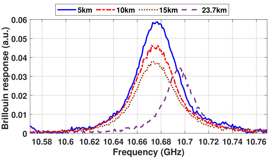 Figure 11
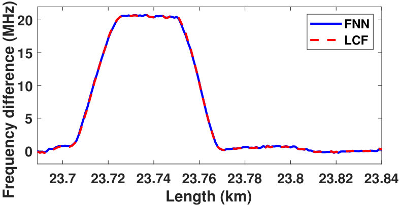 Figure 12
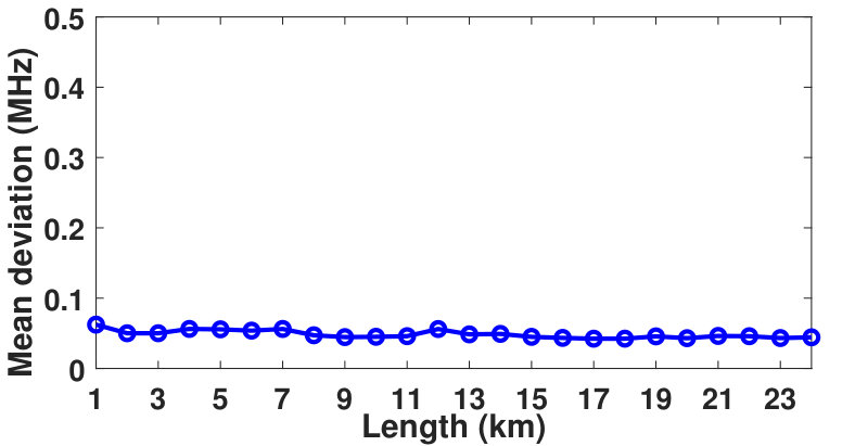 Figure 13
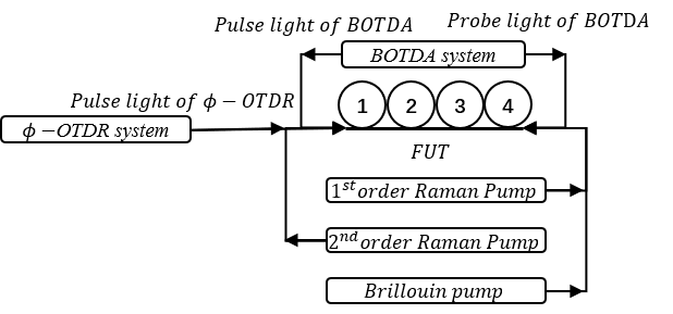 Figure 14
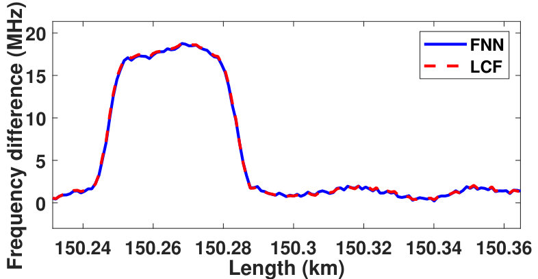 Figure 15
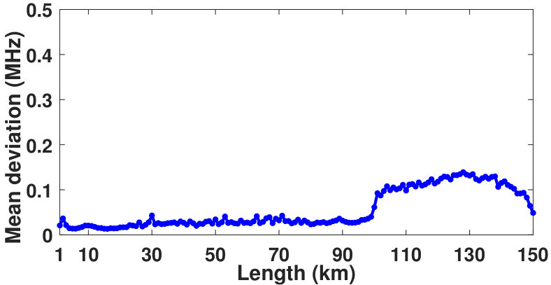 Figure 16
 Figure 2
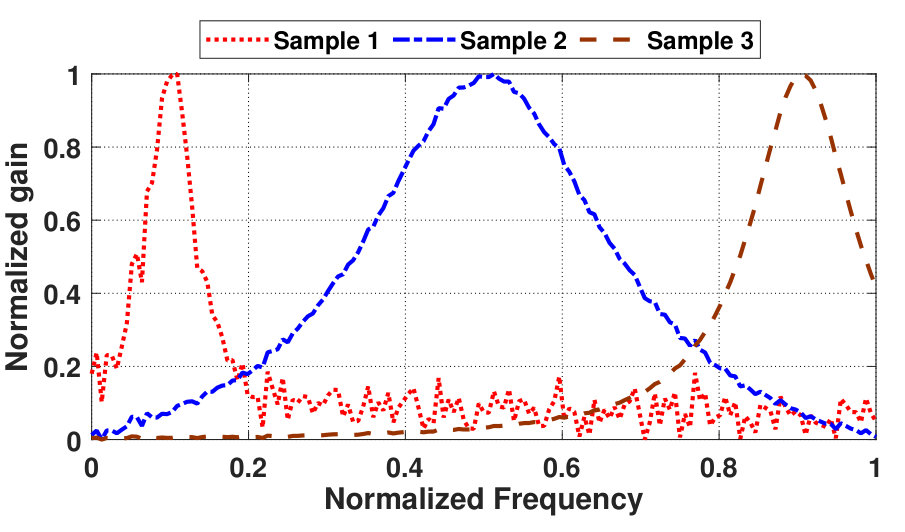 Figure 3
 Figure 4
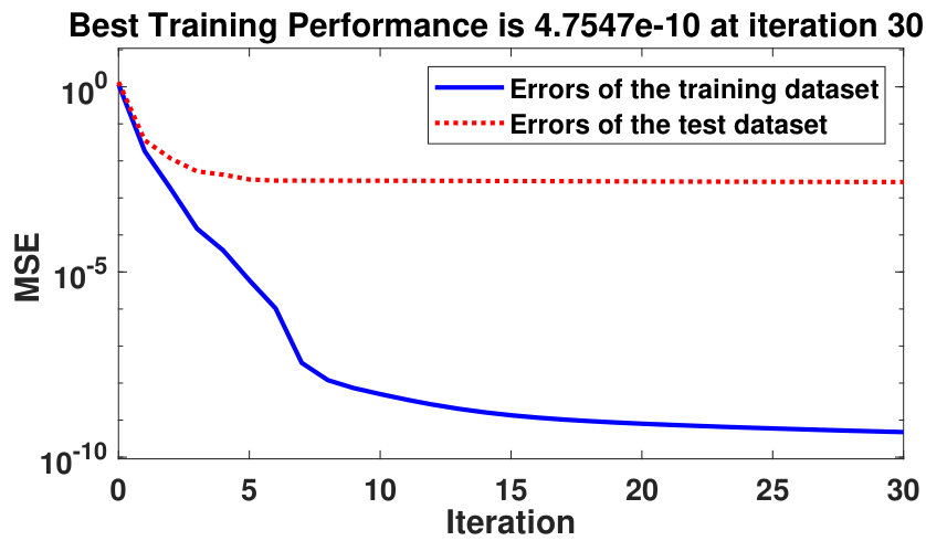 Figure 5
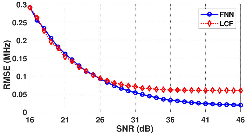 Figure 6
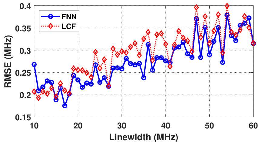 Figure 7
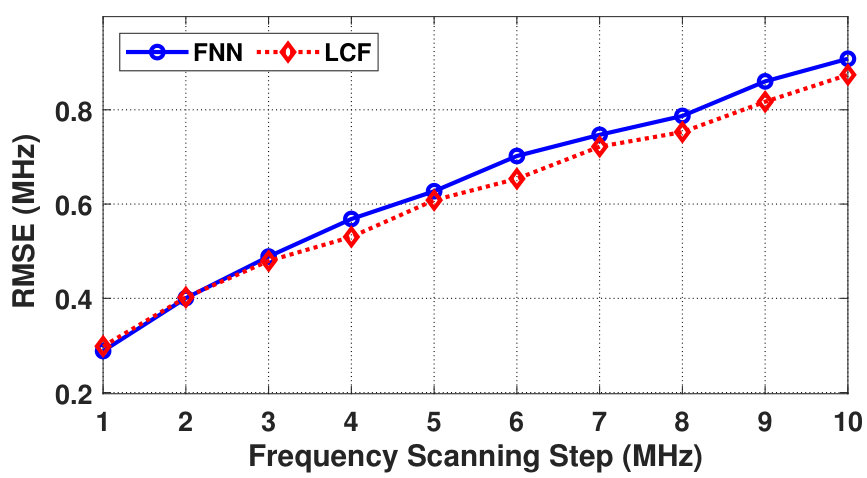 Figure 8
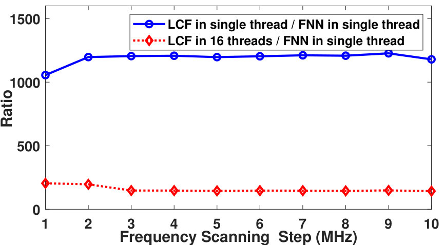 Figure 9
Peer Reviews
No public reviews on file for this paper yet. If you reviewed it on a platform where reviews are public (OpenReview, ICLR, NeurIPS, ICML), you can paste yours below so the community can read it here.
Videos
No videos yet. Explain this paper in a talk, walkthrough, or lecture? Add one.
Taxonomy
TopicsAdvanced Fiber Optic Sensors · Advanced Optical Sensing Technologies · Non-Invasive Vital Sign Monitoring
Optimized Feedforward Neural Network Training for Efficient Brillouin Frequency Shift Retrieval in Fiber
Yongxin Liang1, Jialin Jiang1, Yongxiang Chen1, Richeng Zhu1, Chongyu Lu1, and Zinan Wang1, 2 1Key Lab of Optical Fiber Sensing and Communications, University of Electronic Science and Technology of China, Chengdu, Sichuan, China 611731. 2Center for Information Geoscience, University of Electronic Science and Technology of China, Chengdu, Sichuan, China 611731 This work is supported by Natural Science Foundation of China (41527805, 61731006), Sichuan Youth Science and Technology Foundation (2016JQ0034), Guofang Keji Chuangxin Tequ, and the 111 project (B14039). Corresponding author: Zinan Wang (e-mail: [email protected]).
Abstract
Artificial neural networks (ANNs) can be used to replace traditional methods in various fields, making signal processing more efficient and meeting the real-time processing requirements of the Internet of Things (IoT). As a special type of ANN, recently the feedforward neural network (FNN) has been used to replace the time-consuming Lorentzian curve fitting (LCF) method in Brillouin optical time-domain analysis (BOTDA) to retrieve the Brillouin frequency shift (BFS), which could be used as the indicator in temperature/strain sensing, etc. However, FNN needs to be re-trained if the generalization ability is not satisfactory, or the frequency scanning step is changing in the experiment. This is a cumbersome and inefficient process. In this paper, FNN only needs to be trained once with the proposed method. 150.62 km BOTDA is built to verify the performance of the trained FNN. Simulation and experimental results show that the proposed method is promising in BOTDA because of its high computational efficiency and wide adaptability.
Index Terms:
Feedforward neural networks, Brillouin optical time-domain analysis, Lorentzian curve fitting, Sensor fusion, Optical fiber sensors.
I Introduction
The Internet of Things (IoT) is constantly progressing as multiple technologies are evolving, especially the sensing technologies[1, 2, 3, 4, 5]. As an important branch of sensors, optical fiber sensors, have been studied by many researchers due to their unique advantages[6]. Particularly, distributed optical fiber sensing (DOFS) systems are of great interests since they can turn fiber cables into massive sensor arrays[7, 8, 9, 10]. Brillouin optical time-domain analysis (BOTDA) system is an important type of DOFS, which could achieve high precision, long distance and fast scan-rate sensing [11, 12, 13, 14].
The stimulated Brillouin scattering (SBS) effect is the basis of BOTDA[15, 16]. In BOTDA, usually pump pulse and continuous-wave (CW) probe light are counter-propagating inside the fiber to sample the Brillouin gain spectrum (BGS), then the Brillouin frequency shift (BFS) is retrieved for the purpose of temperature/strain sensing. Before the traditional Lorentzian curve fitting (LCF) method is used to find the BFS[17], the non-local means (NLM), wavelet denoising (WD) or block-matching and 3D filtering (BM3D) can be used to reduce the noise of the BGS in general[18]. All of those processes are time-consuming operations, especially for longer sensing distance and finer spatial resolution. Recently, denoise convolutional neural network (DnCNN) is used for BOTDA filtering [19], which can achieve real-time filtering as long as the DnCNN is trained properly. However, the training process of DnCNN is complicated.
On the other hand, artificial neural networks(ANNs) have been applied in BOTDA[20, 21, 22]. As a special type of ANN, the feedforward neural network (FNN) can be used to replace the traditional LCF method and improve the processing speed. Ideal BGSs are used for FNN training[20]. During FNN testing process, the noise in the measured BGS needs to be reduced as much as possible, which means that the filtering operation cannot be omitted. However, using traditional filtering methods will not meet the requirements of real-time analysis. Although using DnCNN can achieve fast filtering, the training process is complicated. Without filtering, it means that FNN trained by ideal BGSs may not have generalization ability for the noisy BGS in the experiment. Regularization method is needed in order to enhance the generalization ability of FNN[23, 24, 25]. This is a time-consuming task.
Also, the frequency scanning step is one of the key parameters in BOTDA operation. It usually varies between 1 MHz and 10 MHz depending on the required accuracy and speed of the measurement. Previous work required training different FNNs to meet the needs of different frequency scanning steps, which is a tedious task.
In this paper, optimized FNN training method is proposed for BOTDA. As a result, BFS retrieval from the BGSs can be efficiently carried out with a wide range of BGS linewidths, signal-to-noise ratios (SNRs) and frequency scanning steps. The results show that the accuracy of FNN is similar to LCF, while FNN is much faster than LCF. The 23.95 km and 150.62 km BOTDA at the frequency step of 1 MHz and 4 MHz are established respectively to experimentally verify the performance of FNN.
This paper is organized as follows. Section II describes the principles of LCF and FNN to get BFS from BGSs. Section III describes FNN training process and the results. Section IV explains how to enhance the adaptability of the trained FNN. Section V presents the experiment and analyses the results. Section VI gives the conclusion.
II The principles of LCF and FNN
The principles for BFS retrieval from the BGSs using LCF and FNN are explained respectively in this section.
II-A The principle of LCF
In BOTDA, the obtained local BGS conforms to the shape of Lorenz curve. Equation (1) is the core of BGSs simulation.
[TABLE]
where is the linewidth. is the position of the fiber. is the gain coefficient. is the scanning frequency. is the measured BGS. is BFS which reflects information about temperature or strain. The fiber is placed in a stable environment so that the change of BFS is only caused by temperature theoretically:
[TABLE]
where is the temperature coefficient. Temperature difference can be obtained by measuring the difference of BFS. In order to obtain BFS, the least squares estimation (LSE) method is used in LCF.
[TABLE]
The purpose of (3) is to minimize the by modifying parameters during iterations. At the end of the iteration, y is the result of LCF.
II-B The principle of FNN
The hidden layer of FNN is set according to the size of training data and the number of input and output nodes. A typical FNN is showed in Fig 1.
The number of the input layer, the hidden layer, and the output layer are , and , respectively. The input and output of the FNN are and , respectively. The input and output of the hidden layer are and , respectively. The weight from to and to are and , respectively. The FNN accepts a vector of length as the input data, and finally generates a vector of length as the output data. The input of the hidden layer in the iteration is:
[TABLE]
The output of the hidden layer is:
[TABLE]
where · is the sigmoid function. The output of the network is:
[TABLE]
[TABLE]
The expected output of the network is:
[TABLE]
The error signal in the iteration is defined as:
[TABLE]
And the cost function can be defined as:
[TABLE]
In order to minimize the error, the basic method is to use the steepest descent algorithm for backpropagation (BP) calculations, which modifies the weight according to (11) and (12). Besides, there are other algorithms, such as conjugate gradient algorithm, Levenberg-Marquardt(LM) algorithm and so on.
[TABLE]
[TABLE]
The input vector is the local BGS, and the output vector is BFS of the local BGS. It should be noted that both the input local BGS and the output BFS need to be normalized. The reason for the input local BGS needed to be normalized is that as the sensing distance increases, the gain of the local BGS decreases, and the normalization operation eliminates the effects of different gains. Besides, it is convenient to calculate the actual BFS in different parameters among experiments when the output BFS is normalized. The training process of FNN is showed in Fig. 2.
This section provides the principles for BFS retrieval by these two methods. As a traditional method, LCF has a guaranteed accuracy but a time-consuming process, while FNN has the ability to calculate quickly but requires verification of accuracy.
III OPTIMIZED FNN TRAINING: SIMULATION RESULTS
Training a FNN with good generalization ability is not an easy task. Using the optimized training process of adding noise to ideal BGSs method can improve the generalization ability of FNN[26]. It will be described in this section.
Generally, in BOTDA, the measured BGS needs to be scanned in a wide frequency range to find the location of BFS. Here, 156 MHz frequency scanning range at the frequency scanning step of 1 MHz is selected so that the input data of the neural network is a vector of length 157. The layout of hidden layers is set to 40-15 after several attempts. Therefore, the layout of FNN is 157-40-15-1. The size of simulated BGSs is 157×385560, which satisfies the linewidths range from 10 MHz to 60 MHz at a step of 1 MHz, and the BFS varies from 10% to 90% in the 156 MHz frequency range at a step of 1 MHz. In addition, it also contains BGSs under different power noises.
The addition of random noise to training data can enhance the generalization ability of FNN. Therefore, the simulated BGSs with several SNRs are generated to train FNN. The range of SNRs is 16 dB to 36 dB at a step of 10 dB. 20 sets of random noise are added to the ideal BGS in each SNR. Three samples are selected from all simulated BGSs for observation and showed in Fig. 3.
The simulated 16 dB BGSs with different linewidths are used as the test dataset in FNN training process. Using the LM training algorithm, the training process takes about 9 hours in 30 iterations. As shown in Fig. 4, the error of the training and test dataset has the same order of magnitude at the iteration, which means that the trained FNN has generalization ability for the 16 dB BGSs.
For comparison, the simulated BGSs without noise are used as the training dataset. Other simulation and training parameters are consistent, and the error results are showed in Fig. 5. The error of the training and test dataset has different orders of magnitude at the iteration, which means that the trained FNN cannot retrieve the BFS from the 16 dB BGSs accurately. The error of the training dataset is driven to a small value while the error of the test dataset still in a high level, which means the overfitting occurs.
Through this optimized training process of noise addition, the trained FNN has good generalization ability and greatly improves the training efficiency without additional regularization methods. The trained FNN can be used to calculate BFS directly.
Next, the simulated BGSs with different SNRs from 16 dB to 46 dB at a step of 1 dB are used for test. The root-mean-square error (RMSE) of BFS is calculated by FNN and LCF, respectively. The result is showed in Fig. 6.
Fig. 6 shows that the RMSE of BFS calculated by FNN and LCF from the BGS with lower SNR is similar. With the increase of SNR, the RMSE calculated by FNN can be reduced to below 0.05 MHz, while the error of LCF is always above 0.05 MHz. Besides, the simulated 16 dB BGSs with different linewidths at a frequency scanning step of 1 MHz are used for test, as shown in Fig. 7.
Through the optimized training method, a FNN that can calculate BFS accurately from the BGSs with different linewidths and SNRs is trained.
IV THE FNN ADAPTABILITY: SIMULATION RESULTS
The FNN trained in the previous section will not be available if the frequency scanning step is not 1 MHz in the experiment, which means that the BGSs at the corresponding frequency scanning step are needed to be simulated again and used as the training dataset to train another FNN. In long distance BOTDA, it is more desirable to use a higher frequency scanning step, such as 4 MHz. This will increase the measured speed of the BGS at the expense of the accuracy of the temperature measurement. Correspondingly, a lower frequency scanning step, such as 1 MHz, is selected under high precision requirements. Training different FNNs using the BGSs at different frequency scanning steps can be used to solve this issues.
However, the FNN training is a cumbersome process that involves generating simulated data, adjusting hidden layers and other parameters until the FNN has generalization ability and satisfactory error results. Therefore, it will be convenient if only one FNN needs to be trained, which can retrieve BFS from BGS at different frequency scanning steps. In order to solve this issue, the linear interpolation method can be used to reshape the other frequency scanning step of the BGS to 1 MHz.
Consistency is required to obtain accurate results. The frequency scanning range should not be lower than 156 MHz because the previous FNN is trained using simulated BGSs with the frequency scanning range of 156 MHz. In order to ensure the frequency scanning range is an integer multiple of the frequency scanning step, the minimum frequency scanning ranges at different frequency scanning steps are different. They are at least 156 MHz, 156 MHz, 156 MHz, 156 MHz, 160 MHz, 156 MHz, 161 MHz, 160 MHz, 162 MHz, 160 MHz, corresponding to different frequency scanning steps from 1 MHz to 10 MHz at a step of 1 MHz. The linear interpolation is used to reshape the BGS to the frequency scanning step of 1 MHz. At last, the interpolated BGS in appropriate frequency scanning range of 156 MHz is selected and input into the FNN to retrieve the BFS.
The BFS is retrieved by FNN and LCF from the 16 dB BGSs with different linewidths at the different frequency scanning steps, and the result of the RMSE is showed in Fig. 8. The error of FNN and LCF is basically same. Both of them are small compared with the measurement uncertainty in the experiment.
In order to compare efficiency, the BFS is retrieved by FNN and LCF from 10,000 sets of the local BGS at each frequency scanning step. The consumption time ratios of LCF (single thread and 16 threads) to FNN (single thread) is showed in Fig. 9.
The interpolation method enables BGSs at different frequency scanning steps to be input into a trained FNN and then obtain the accurate BFS calculation. The high efficiency and wide adaptability of FNN will promote the development of BOTDA.
V EXPERIMENTAL DEMONSTRATION
In order to analyze the ability of the FNN for calculating the BFS from the BGS in the experiment, the 23.95 km BOTDA with 200 MHz frequency range at a frequency scanning step of 1 MHz and 150.62 km BOTDA with 156 MHz frequency range at a frequency scanning step of 4 MHz are established, respectively.
V-A Experimental setup of the 23.95 km BOTDA
The experimental setup of the 23.95 km BOTDA is showed in Fig. 10. This is a typical BOTDA experimental system. Pump pulse and CW probe light are counter-propagating inside the fiber under test (FUT) to sample the BGS. The BGS is measured by direct detection in the frequency scanning range of 200 MHz, with the frequency scanning step of 1 MHz.
The heating location is at 23.7 km. The SNR is 23.5 dB, approximately. As can be seen from Fig. 11, the position of the BFS is changed due to heating.
The input of the FNN is the local BGS in the frequency scanning range of 156 MHz at a frequency scanning step of 1 MHz. However, the frequency scanning range of the measured BGS is 200 MHz at a frequency scanning step of 1 MHz. Therefore, the BGS with appropriate 156 MHz frequency range is selected according to the position of the power peak and input to the neural network to retrieve the BFS. Also, the BFS is calculated by LCF for comparison. Subtracting BFS before and after heating to obtain the frequency difference, which reflects the change of temperature, as shown in Fig. 12. The temperature coefficient is 1.3 MHz/∘C and the applied temperature difference is 15.7∘C. The temperature difference measured by LCF and FNN are both 15.6∘C. The measurement uncertainty calculated by LCF and FNN are 0.22∘C and 0.23∘C, respectively.
Themean deviation of the frequency difference of BFS calculated by FNN and LCF is analyzed every 1 km, as shown in Fig. 13. Compared to LCF, it indicates that FNN can accurately calculate BFS from the BGS.
V-B Experimental setup of the 150.62 km BOTDA
To further analyze the performance of the FNN, an advanced BOTDA of 150.62 km is built. The spatial resolution is 9 m, which means sixteen thousand sensing units are fused along the fiber to sense the change of temperature. A variety of technologies, such as hybrid distributed amplification, frequency division multiplexing (FDM), wavelength division multiplexing (WDM), time division multiplexing (TDM), are combined and used in the experiment[11]. The experimental setup is showed in Fig. 14. The frequency scanning step of the BGS is 4 MHz and the frequency scanning range is 156 MHz.
The SNR of the BGS of the four-segment fiber is analyzed. The first three segments have the same SNR, about 27 dB, and the last segment is about 18 dB.
Since the frequency scanning step is 4 MHz, linear interpolation is required to reshape the BGS before it is input to the FNN. The frequency difference of BFS calculated by FNN is compared with LCF, as shown in Fig. 15. The temperature coefficient is 1.0 MHz/℃ and the applied temperature difference is 18.2 ℃. The temperature difference measured by LCF and FNN are both 18.7 ℃. The measurement uncertainty calculated by LCF and FNN are ±0.82 ℃ and ±0.83 ℃, respectively. T he measurement uncertainty is higher than the 23.95 km BOTDA at a frequency scanning step of 1 MHz.
Similarly, the mean deviation of the frequency difference of BFS calculated by FNN and LCF is analyzed every 1 km, as shown in Fig. 16. It is acceptable that the mean deviation is less than 0.2 MHz compared with the measurement uncertainty.
By constructing and analyzing BOTDA experiments, it confirms that FNN can retrieve BFS accurately under different experimental parameters.
VI Conclusion
Using the proposed FNN training method, BFS can be retrieved from the BGSs under various experimental parameters. Compared with LCF, FNN trained with the proposed method is much more efficient, without sacrificing the measurement uncertainty. This work proves the value of FNN in DOFS system and promotes the development of DOFS for real-world applications.
The reference list from the paper itself. Each links out to its DOI / PubMed record.
- 1[1] A. Zanella, N. Bui, A. Castellani, L. Vangelista, and M. Zorzi, “Internet of Things for Smart Cities,” IEEE Internet of Things Journal , vol. 1, no. 1, pp. 22–32, Feb. 2014.
- 2[2] E. Hodo, X. Bellekens, A. Hamilton, P. Dubouilh, E. Iorkyase, C. Tachtatzis, and R. Atkinson, “Threat analysis of Io T networks using artificial neural network intrusion detection system,” in 2016 International Symposium on Networks, Computers and Communications (ISNCC), Hammamet,Tunisia , May. 2016, pp. 1–6.
- 3[3] H. Cai, B. Xu, L. Jiang, and A. V. Vasilakos, “Io T-Based Big Data Storage Systems in Cloud Computing: Perspectives and Challenges,” IEEE Internet of Things Journal , vol. 4, no. 1, pp. 75–87, Feb. 2017.
- 4[4] T. Yashiro, S. Kobayashi, N. Koshizuka, and K. Sakamura, “An Internet of Things (Io T) architecture for embedded appliances,” in 2013 IEEE Region 10 Humanitarian Technology Conference, Sendai, Japan , Aug. 2013, pp. 314–319.
- 5[5] J. Gubbi, R. Buyya, S. Marusic, and M. Palaniswami, “Internet of Things (Io T): A vision, architectural elements, and future directions,” Future Generation Computer Systems , vol. 29, no. 7, pp. 1645–1660, Sept. 2013.
- 6[6] D. A. Krohn, T. Mac Dougall, and A. Mendez, Fiber optic sensors: fundamentals and applications . in SPIE Press, 4th ed. Bellingham, WA, USA: SPIE, 2014.
- 7[7] P. Ferdinand, “The evolution of optical fiber sensors technologies during the 35 last years and their applications in structure health monitoring,” in EWSHM-7th European Workshop on Structural Health Monitoring , Jul. 2014. [Online]. Available: https://hal.inria.fr/hal-01021251
- 8[8] Z. Wang, B. Zhang, J. Xiong, Y. Fu, S. Lin, J. Jiang, Y. Chen, Y. Wu, Q. Meng, and Y. Rao, “Distributed acoustic sensing based on pulse-coding phase-sensitive OTDR,” IEEE Internet of Things Journal , Sept. 2018. [Online]. Available: https://dx.doi.org/10.1109/JIOT.2018.2869474