Optimality Clue for Graph Coloring Problem
Alexandre Gondran (ENAC), Laurent Moalic (Universit\'e de Haute-Alsace, (UHA))

TL;DR
This paper introduces a novel method called optimality clue that uses randomized heuristics to estimate the likelihood of a solution being optimal in the Graph Coloring Problem, validated on benchmark instances.
Contribution
It presents a new approach to verify solution optimality in GCP by estimating the number of colorings using randomized heuristics, enabling practical optimality proofs.
Findings
Effective in confirming optimality on benchmark instances
Provides a probabilistic upper bound for the number of colorings
Works with standard heuristics like HEAD for large graphs
Abstract
In this paper, we present a new approach which qualifies or not a solution found by a heuristic as a potential optimal solution. Our approach is based on the following observation: for a minimization problem, the number of admissible solutions decreases with the value of the objective function. For the Graph Coloring Problem (GCP), we confirm this observation and present a new way to prove optimality. This proof is based on the counting of the number of different k-colorings and the number of independent sets of a given graph G. Exact solutions counting problems are difficult problems (\#P-complete). However, we show that, using only randomized heuristics, it is possible to define an estimation of the upper bound of the number of k-colorings. This estimate has been calibrated on a large benchmark of graph instances for which the exact number of optimal k-colorings is known. Our…
Click any figure to enlarge with its caption.
 Figure 1
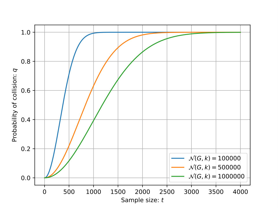 Figure 2
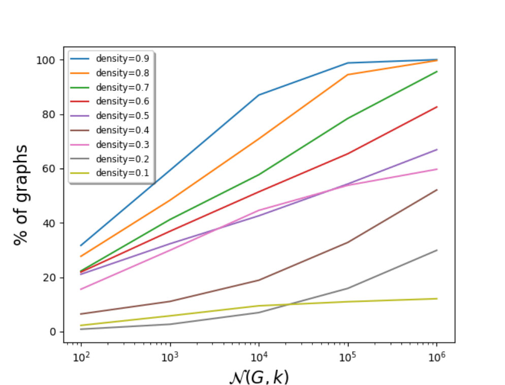 Figure 3
 Figure 4
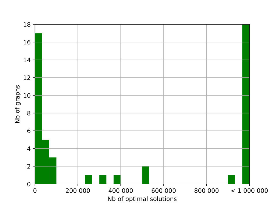 Figure 5
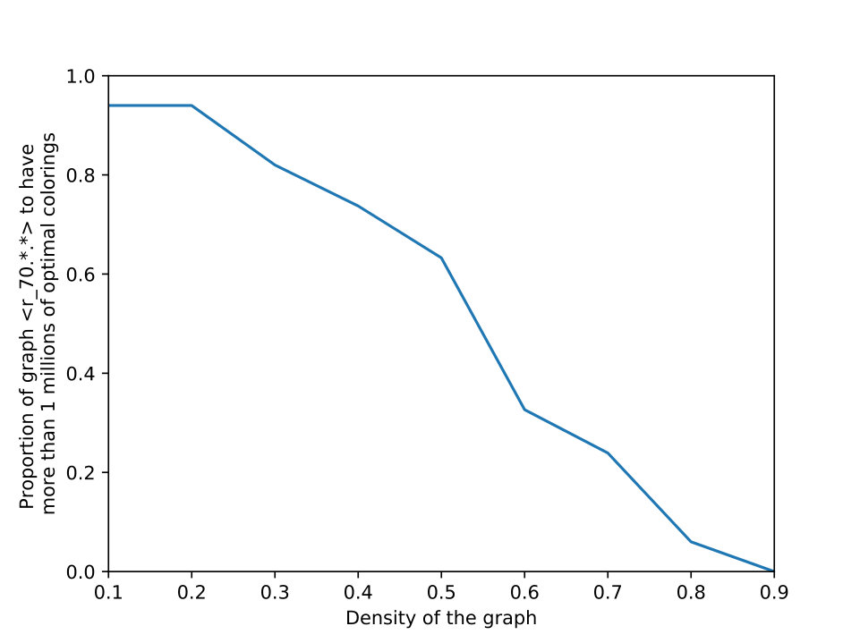 Figure 6
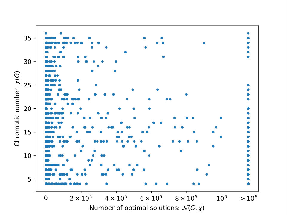 Figure 7
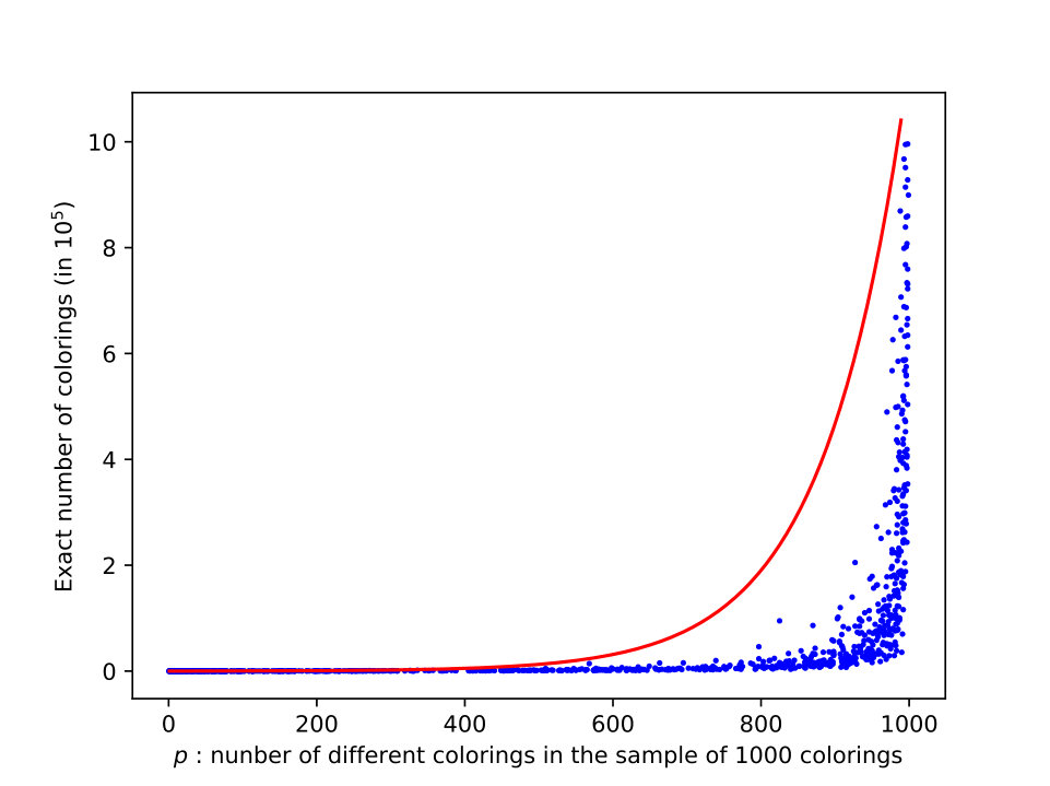 Figure 8
 Figure 9
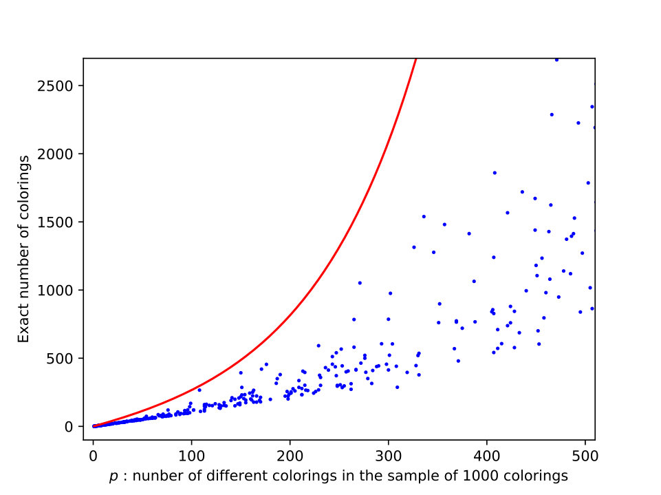 Figure 10
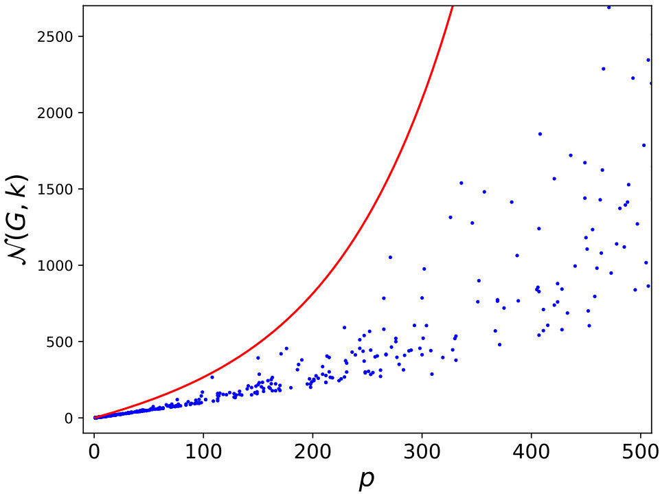 Figure 11
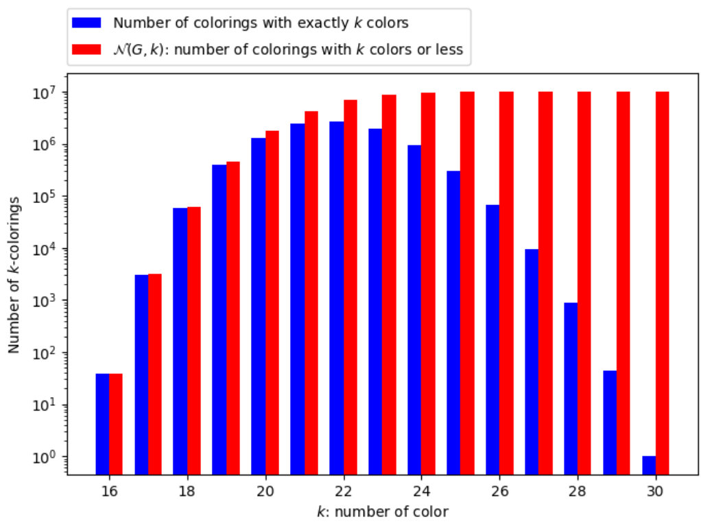 Figure 12
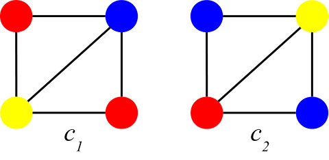 Figure 13
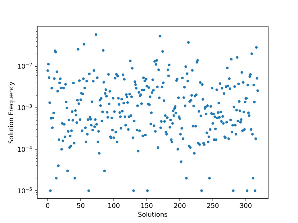 Figure 14
| known | Total | |||||||
| ? | #instances | |||||||
| 862 (control dataset) | 959 (reference dataset) | 210 (test dataset) | 2031 | |||||
| 393 | 566 | |||||||
| opt. clue | not opt. clue | opt. clue | not opt. clue | opt. clue | not opt. clue | opt. clue | not opt. clue | |
| 0 | 862 | 0 | 393 | 449 | 117 | 39 | 171 | |
| Instances | Opt. clue | time (s) | time(s)[15] | ||||||||||
| DSJC125.5 | 125 | 0.5 | 17 | 17 | 537,508 | ? | 1,000 | 767 | 141,503 | True | 161 | 17 | 274 |
| DSJC125.9 | 125 | 0.9 | 44 | 44 | 1,249 | ? | 1,000 | 998 | False | 28 | 44 | 7 | |
| DSJC250.9 | 250 | 0.9 | 72 | 72 | 6,555 | ? | 1,000 | 889 | 423,733 | False | 1,963 | 72 | 11,094 |
| flat1000_50_0 | 1,000 | 0.49 | 50 | 50 | ? | 1,000 | 1 | 2 | True | 25,694 | 50 | 3,331 | |
| flat1000_60_0 | 1,000 | 0.49 | 60 | 60 | ? | 1,000 | 1 | 2 | True | 44,315 | 60 | 29,996 | |
| le450_5a | 450 | 0.06 | 5 | 5 | 32 | 1,000 | 32 | 69 | True | 60 | 5 | <0.1[21] | |
| le450_5b | 450 | 0.06 | 5 | 5 | 1 | 1,000 | 1 | 2 | True | 138 | 5 | <0.1[21] | |
| le450_5c | 450 | 0.1 | 5 | 5 | 1 | 1,000 | 1 | 2 | True | 28 | 5 | <0.1[21] | |
| le450_5d | 450 | 0.1 | 5 | 5 | 8 | 1,000 | 8 | 16 | True | 20 | 5 | <0.1[21] | |
| le450_15c | 450 | 0.17 | 15 | 15 | ? | 1,000 | 919 | 554,866 | True | 15 | <0.1[21] | ||
| le450_15d | 450 | 0.17 | 15 | 15 | ? | 1,000 | 579 | 26,041 | True | 15 | <0.1[21] | ||
| myciel3 | 11 | 0.36 | 4 | 4 | 102 | 520 | 1,000 | 435 | 7,105 | False | 10 | 4 | <0.1 |
| queen5_5 | 25 | 0.53 | 5 | 5 | 461 | 2 | 1,000 | 2 | 4 | True | 9 | 5 | <0.1[21] |
| queen6_6 | 36 | 0.46 | 7 | 7 | 2,634 | 20 | 1,000 | 20 | 42 | True | 10 | 7 | <0.1 |
| queen7_7 | 49 | 0.4 | 7 | 7 | 16,869 | 4 | 1,000 | 4 | 8 | True | 10 | 7 | <0.1[21] |
| queen8_8 | 64 | 0.36 | 9 | 9 | 118,968 | 154,068 | 1,000 | 993 | False | 11 | 9 | <1 | |
| r125.1c | 125 | 0.97 | 46 | 46 | 787 | ? | 1,000 | 977 | 934,514 | False | 5,962 | 46 | <0.1[21] |
| DSJC250.5 | 250 | 0.5 | ? | 28 | 24,791,612 | ? | 1,000 | 999 | False | 1,696 | 26 | 18 | |
| DSJC500.5 | 500 | 0.5 | ? | 47 | ? | 341 | 281 | 32,731 | True | out of time | 43 | 439 | |
| 48 | ? | 100,000 | 100,000 | False | |||||||||
| DSJC500.9 | 500 | 0.9 | ? | 126 | 35,165 | ? | 1,000 | 927 | 59,623 | False | 234,496 | 123 | 100 |
| DSJC+300.1_8 | 300 | 0.1 | ? | 8 | ? | 1,000 | 3 | 6 | True | 22,896 | 5 | <0.1[21] | |
| DSJC+300.5_31 | 300 | 0.5 | ? | 31 | ? | 1,000 | 2 | 4 | True | 69,363 | 29 | 20 | |
| DSJC+400.5_39 | 400 | 0.5 | ? | 39 | ? | 1,000 | 96 | 252 | True | 386,037 | 36 | 135 |
Peer Reviews
No public reviews on file for this paper yet. If you reviewed it on a platform where reviews are public (OpenReview, ICLR, NeurIPS, ICML), you can paste yours below so the community can read it here.
Videos
No videos yet. Explain this paper in a talk, walkthrough, or lecture? Add one.
Taxonomy
TopicsVehicle Routing Optimization Methods · Scheduling and Timetabling Solutions
Optimality Clue for Graph Coloring Problem
Alexandre Gondran
ENAC
French Civil Aviation University
Toulouse
France
Laurent Moalic
UHA
University of Upper Alsace
Mulhouse
France
Abstract
In this paper, we present a new approach which qualifies or not a solution found by a heuristic as a potential optimal solution. Our approach is based on the following observation: for a minimization problem, the number of admissible solutions decreases with the value of the objective function. For the Graph Coloring Problem (GCP), we confirm this observation and present a new way to prove optimality. This proof is based on the counting of the number of different -colorings and the number of independent sets of a given graph .
Exact solutions counting problems are difficult problems (#P-complete). However, we show that, using only randomized heuristics, it is possible to define an estimation of the upper bound of the number of -colorings. This estimate has been calibrated on a large benchmark of graph instances for which the exact number of optimal -colorings is known.
Our approach, called optimality clue, build a sample of -colorings of a given graph by running many times one randomized heuristic on the same graph instance. We use the evolutionary algorithm HEAD [26], which is one of the most efficient heuristic for GCP.
Optimality clue matches with the standard definition of optimality on a wide number of instances of DIMACS and RBCII benchmarks where the optimality is known. Then, we show the clue of optimality for another set of graph instances.
keywords:
Optimality Metaheuristics Near-optimal.
1 Introduction
For a given integer , a -coloring of a given graph is an assignment of one of distinct colors to each vertex in the graph, so that no two adjacent vertices (linked by an edge ) are given the same color. The Graph Coloring Problem (GCP) is to find, for a given graph , its chromatic number corresponding to the smallest such that there exists a -coloring of . GCP is NP-hard [19] for . The -coloring problem (-CP) is the associated decision problem. For an optimization problem which is NP-hard, there is no efficient polynomial-time exact algorithm to solve it, unless PNP. Therefore for large size instances of a minimization NP-hard problem, the exact algorithms must be stopped before their end. In this case, exact algorithms such as branch and bound methods find a lower bound of the optimal value of the objective function. Heuristic approaches are then the only ways to find, in reasonably fast running-time, a “good” solution in terms of objective function value, i.e. an upper bound of the optimal value. However, even if an admissible solution is found, its distance to the optimal solution remains unknown, except for approximation algorithms111Notice that it is still NP-hard to approximate within for any [35].. The optimality gap is the different between the upper bound (found by a heuristic) and the lower bound (found by a partial exact method). Optimality is proven only when this gap is equal to zero. Unfortunately for large size instances of an NP-hard problem, this gap is often important. It is particularly true for challenging instances [15, 26] of the GCP of the DIMACS benchmark [18]. This paper addresses the following question: What to do in this situation? Is it possible to prove optimality of a graph coloring problem instance using only heuristic algorithms?
The response is Yes, for specific class of graphs: for example, it exists efficient polynomial-time exact algorithms to find for interval graphs, chordal graphs, cographs [27, 31]. For some graphs like 1-perfect graphs222A perfect graph is a graph in which the chromatic number of every induced subgraph equals the size of the largest clique of that subgraph. 1-perfect graphs are more general than perfect graphs. There exists polynomial-time exact algorithms to find for perfect graphs [13], but slow in practice. Line graphs, chordal graphs, interval graphs or cographs are subclasses of perfect graphs., for which the chromatic number is equal to the size of the maximum cliques , it is possible to solve the dual problem, the Maximum Clique Problem (MCP), with another heuristic and conclude to optimality if the size of the maximum clique found is equal to the smallest number of colors used for coloring found also by a heuristic. In this specific case, the optimality gap (or duality gap between GCP and MCP) is zero.
However, the response to the question is No, in general case; a heuristic finds approximate solutions (upper bound); although the coloring found may be optimal, it is not possible to prove this possible optimality. Therefore, the question become: what can be done better using only a heuristic than finding an approximate solution? Is it possible to define a kind of optimality index for a graph coloring problem instance?
One shows in this article that a heuristic does not only find an upper bound of but that it is also able to count the number of different -colorings (i.e. the number of admissible solutions having the same objective function value). Our approach is based on the fact that the number of different -colorings decreases dramatically when the number of colors, , decreases too. Indeed figure 2 gives a typical example of a random graph with 30 vertices, a density of and . The number of colorings with exactly colors (blue bars) and the total colorings with colors or less (red bars), noted , are exactly computed for all values from to . decreases exponentially when decreases to . One proves a theorem showing that when the number of -colorings is lower than a given value (the number of independent sets of 333An independent set is a subset of vertices of , such that every two distinct vertices in the independent set are no adjacent.), then we achieve the optimum: .
In this article, we try to apply the proposed theorem in order to prove optimality.
Brief solutions counting review
Our work tackles the problem of counting solutions of NP-complete problems which has been widely studied for boolean SATisfiability problem, called #SAT, or Constraint Satisfaction Problem (CSP), called #CSP; -coloring problem is a special case of CSP. These problems are known as #P-complete [33]. A recent survey on #CSPs is done in [17]. Even if a problem is not NP-hard, the problem of solutions counting is often hard. Specific studies on counting solutions of -CP are done in [16, 7, 25]. Because the exact counting is in many cases a complex problem, statistical or approximate counting are often considered. Then, uniform sampling of the set of solutions problem is related to the problem of counting solutions. Many works are done on uniform or near uniform sampling like [11, 12, 34]. The objective is to count by sampling. Frieze and Vigoda [8] give a survey on the use of Markov Chain Monte Carlo algorithms for approximately counting the number of -colorings. The features of ergodicity or quasi-ergodicity of the heuristics that guarantee an uniform sampling are deeply discussed in [6]. However, theoretical results are obtained with a high value of where is the maximum degree of the graph which is very far from for challenging graphs. On the other hand, when tests are performed with like in [7], the considered graph instances are often with more than -colorings. If the number of -colorings is too high (higher than the number of independent sets), then it is not possible to apply our theorem. Therefore, in practice, our approach can be applied to graphs that do not have too many optimal colorings; we considered graphs with at most 1 million different optimal colorings.
To our knowledge, it is the first time that solutions counting are used to prove optimality. We define a procedure, called optimality clue, in order to apply the proposed theorem. First, we build a sample of -colorings of a given graph by running many times (about 1,000 times) the same randomized heuristic algorithm. In this study, we use HEAD444Open-source code available at: github.com/graphcoloring/HEAD, our open-source memetic algorithm (i.e. hybridization of tabu search and evolutionary algorithm), which is very efficient heuristic solving GCP [26].
In this sample some colorings may appear several times and others only ones. The number of different -colorings inside the sample is used to build an estimation of the total number of colorings with colors. This estimator has been calibrated on a large benchmark of graph instances for which the number of optimal -colorings is exactly known. Because we have no guarantee that the sampling is uniform, in the general case, therefore we have no guarantee that our estimator is always exact.
Moreover, building a sample of -colorings is time-consuming, then the size of the sample should be “reasonable”. Therefore, graphs for which our optimality clue can be calculated are graphs having not too many optimal -colorings (i.e. about less than one million). Of course it is not possible to known a priori if a given graph has more or less than 1 million optimal colorings. Then, our approach provides a clue that a coloring found by the heuristic is perhaps optimal (positive conclusion) but never denies it (no negative conclusion): in many cases we can not have any conclusion.
This article is organized as follows. In Section 2, we present the new optimality proof for GCP based on solutions counting. Our general approach, called optimality clue, is define in Section 3. In Section 4, we detail how we calculate the estimate of the number of -colorings using benchmark graph instances. Numerical tests and experiments are presented in Section 5. Finally, we conclude in Section 6.
2 Proof of Optimality by solutions counting
Notice that there are different ways to count the -colorings of a given graph . When counting the number of different -colorings, we have to take into account the permutations of the color classes. We consider one -coloring not as an assignment of one color among to each vertex but as a partition of the vertices of the graph into independent sets. An Independent Set (IS) or stable set is a set of vertices of , no two of which are adjacent. Two -colorings and are considered identical if they correspond to the same partition of . The distance between two -colorings that is taken into account is the set-theoretic partition distance used in [10, 14, 26], which is independent of the permutation of the color classes. In previous works about solutions counting of -CP [7], authors counted the total number of -colorings including all the permutations like in the example of Figure 2; such a calculation of the number of different -colorings is times higher than the way we count. This makes their methods inapplicable to our study. We write the set of all -colorings of the graph . A -coloring can use exactly colors or less, then . The cardinal of is noted .
Our approach is based on the following fact :
Lemma 1
Let a graph and an integer . If there exists at least one -coloring of , then there exists at least different -colorings of :
[TABLE]
where is the number of independent sets of .
Proof 2.1**.**
Notice that a -coloring of a graph is a partition of vertices into IS. Indeed vertices colored with the same color inside a -coloring are necessarily an IS. In other words, it is always possible to color all vertices of any IS with the same color. We note the set of all the IS of , then .
Starting with one coloring of with exactly colors, for each independent set of except for the IS of the -coloring, it is possible to recolor all vertices of this independent set with a new color (the th color). We obtain by this way one different -coloring for each different independent set, then we count at least a total of different colorings with exactly colors. Then, because we have to count also the starting -coloring.
Then, we obtain the following theorem:
Theorem 1
Let a graph and an integer . Let the number of -colorings of and the number of independent sets of .
If , then .
Proof 2.2**.**
* because . If , it means that there exists at least one -coloring (i.e. ). If we add a new color, it is possible to consider this -coloring and to recolor any independent set of with the new color, we obtain by this way different -colorings (by Lemma 1). Therefore which refute initial assumption.*
For example, the studied graph in Figure 2 (30 vertices and density 0.9) has 38 different colorings with 16 colors: ; moreover this graph has 78 IS: , then the theorem is applicable with because: . Then, thanks to the theorem we can conclude that . Moreover, for , , so the theorem is not applicable.
Corollary 1
Let a graph and an integer . Let an upper bound of the number of and a lower bound of .
If and , then .
3 Optimality Clue
We propose in this paper to apply the corollary 1, so to find an appropriate upper bound of the number of -colorings of , , and a lower bound of the number of independent sets of , .
3.1 IS counting
There exists many algorithms [4, 5, 28, 30] for counting all the maximal independent sets of a graph (or similarly counting all the maximal cliques555A maximal clique is a clique that cannot be extended by including one more adjacent vertex. A maximum clique is a clique that has the largest size in a given graph; a maximum clique is therefore always maximal, but the converse does not hold. Analogue definition for IS. in , the complementary graph of ). By definition, the number of maximal IS, noted , is a lower bound of . Those algorithms are based on enumeration. Because we focus this study on graphs having less than 1 million optimal solutions, we can stop the enumerating after finding 1 million IS. Generally, is very high except for graphs with very high density. Real-life graphs have often a low density, then is very high. Moreover, a simple lower bound is given by [29] : , where is the size of the largest independent set of and the number of vertices. Bollobás’ book [2] (p.283) gives also a statistical number of maximal cliques of size for a random graph. Then, we conclude that:
[TABLE]
with the number of vertices and the density of a random graph .
In this study, we use Cliquer 666Code available at: users.aalto.fi/ pat/cliquer.html. To count all IS of a graph, you just execute: ./cl ¡complement graph¿ -a -m 1 -M ¡k¿, an exact branch-and-bound algorithm developed by Patric Östergård [28] that enumerates all cliques (an IS is a clique in the complementary graph).
It is more complex to evaluate and section 4 presents a way to build an experimental upper bound of . We characterize this upper bound as experimental because it is based on experimental tests on benchmark graph instances, then there is no total guaranty that it is an upper bound.
3.2 Procedure
We define here the procedure of what we call Optimality Clue for graph coloring: let a graph and a positive integer, that we suspect to be the chromatic number of . The proposed approach is based on the five following steps:
Build a sample of -colorings of : we run the memetic algorithm HEAD on as many times as needed to obtain legal -colorings. Those solutions are the solutions sample. The size of the sample is equal to . We take in general case when it is possible. 2. 2.
Count the number of different -colorings inside the sample. This number is equal to . Of course . 3. 3.
Estimate an upper bound of as (cf. Section 4); this upper bound is function of and . 4. 4.
Compute , the number of IS, or at least a lower bound if , with an exact algorithm (Cliquer). 5. 5.
If , then we conclude that solutions of the sample have a clue to be optimal:
Chances are that is equal to
3.2.1 Uniform sample
If the sample is uniform777All -colorings in the sample are uniformly drawn at random in ., then there exists statistical methods to count solutions and to build an upper bound with statistical guarantee, for example the capture-recapture methods: Peterson method [20], Jolly-Seber method [1] wich is commonly used in ecology to estimate an animal population’s size. However, it is not our case: we have no guarantee that our solutions sample is uniform or near uniform. HEAD is a memetic algorithm that explores the space of non-legal -colorings: a non-legal -coloring is a coloring with at most colors and where two adjacent vertices (linked by an edge) may have the same color (called conflicting edge). The objective of HEAD is to minimize the number of conflicting edges to zero, that is to get a legal -coloring. HEAD is an evolutionary algorithm with a population size equals to two. The two non-legal -colorings perform at each generation a tabu search and after a crossover. The sample distribution depends on the fitness landscape properties [24, 23]888The fitness landscape itself depends on the neighborhood used for tabu search and the crossover used. and there is no reason for this distribution to be uniform. A smooth landscape (respectively a rugged landscape) around a legal -coloring will increase (resp. decrease) the probability of finding this -coloring. Figure 4 represents the frequency of the 319 optimal -colorings of <r140_90.4> graph of RCBII benchmark (140 vertices and density 0.9) in a sample of size 100,000 found by HEAD heuristic. In this typical graph instance, the ratio between the least frequent and the most frequently found coloring is around a factor of which corresponds to the same scale as similar studies [34].
Another approach is to take into account the ergodicity of an algorithm, which is its capability to explore all the search space. More precisely, an algorithm is ergodic if it is possible (probability not null) to reach any -coloring from any other -coloring in a finite number of iterations. Random walks or Metropolis algorithms (with a positive temperature sufficiently high) are ergodic algorithms since there is always a finite probability of escaping from local minimum. However, those algorithms are very inefficient in practice to find an optimal -coloring in the general case.
3.2.2 Sample size
The choice of , the size of the sample, is very important for two reasons. First, in practice, to build a sample of -colorings can be very time-consuming, then the size of the sample should have a reasonable size. We take for most of the graph instances. However, the more challenging the graph instance, the longer HEAD takes to find one -coloring. Therefore, it is not possible to build a sample of size 1,000 for all graphs, such as for the <DSJC500.5> graph of DIMACS (cf. Table 5.1).
The second reason is more theoretical. We have limited the maximum number of different optimal solutions to 1 million, for a graph to be considered by our approach. In fact, we choose 1 million because it equals to with . Indeed, if the sample is uniformly drawn at random in , the probability that at least two colorings of the sample are identical is equal to999This problem is linked to the birthday problem that shows that in a room of just 23 people there’s a 50-50 chance that two people have the same birthday. In our case, the number of days in a year is and the number of people is the size of the sample.: then . We call also the collision probability. So, if then , if then . Figure 4 represents the collision frequency, , in function of the sample size, , for different values of the size. When and , it is almost impossible to miss a collision in the sample, but for , there is around 60% to miss a collision. However, it is not tragic to miss a collision for our approach. Indeed, the consequence is that the clue of optimality may be not applicable but the risk of false positive is avoided. A false positive occurs if our procedure 3.2 improperly indicates the optimality clue, when in reality the -colorings are not optimal. Moreover, the collision frequency is higher for a non-uniform sample than for a uniform one.
4 Estimate of the number of -colorings:
4.1 Data sets
In order to define an estimator or at least an upper bound of the number of -colorings, we need to have a large number of graph instances for which we know the exact number of -colorings. Fabio Furini et al. [9] have published an open-source and very efficient version of the backtracking DSATUR algorithm [3] which returns the chromatic number of a given graph 101010Code available at: lamsade.dauphine.fr/coloring/doku.php. DSATUR is one of the best exact algorithms for GCP, particularly for graphs with high density. We suggest readers interrested in an overview of exact methods for GCP to read [22, 15].
We modified their DSATUR algorithm in order to count the total number of -colorings. The pseudo code of the algorithm, called CDSATUR, is presented in algorithm 1. CDSATUR returns, for all values , the exact value of taking into account the permutation of colors and especially .
Fabio Furini et al. published also 2031 random GCP instances called RCBII 111111Instances available in the same address with vertices from 60 to 140 and density between 0.1 and 0.9. This wide variety of graphs is our reference dataset. We complete this dataset with easy DIMACS graphs [18] for which and is computable with CDSATUR.
The 2031 graphs of RCBII benchmark have characteristics described in Table 1. We can notice that is known for all these graphs [9]. First we calculated with CDSATUR, with a time limit equals to s. This time is enough for most of the graphs. There are only 210 graph instances of RBCII (on the 2031) for which CDSATUR does not have enough time to find . These 210 graphs are used to test our approach (test dataset).
Among the graphs for which can be determined, we consider only those with less than 1 million optimal solutions: they form the reference dataset (959 graph instances). Finally, we can distinct inside the reference dataset, graph instances verifying (566/959) or not (393/959).
It remains 862 graphs on the 2031 of RBCII benchmark with more than 1 million of optimal solutions. We decided to test our approach on those graphs (called control dataset) to check if the proposed algorithm can produce false positives or not.
4.2 Analysis of graph instances
Before determining an upper bound of , we investigate the possible links between standard features of a graph as its size (number of vertices), its density, or its chromatic number and the number of optimal colorings:
4.2.1 Links between , graph size and density
Graphs with same size (number of vertices) and same density can have a number of optimal colorings very different from one another. A typical example is given in Figure 6 where is represented the distribution of 49 graph instances with 80 vertices and density 0.3 (<r80_30.*> of RBCII benchmark) in function of the number of solutions . Half of the graphs (25/49) have less than 100 000 optimal solutions while a third (18/49) have more than 1 million optimal solutions. There are no simple law that characterize this distribution.
However, we can notice that the lower the density, the higher the optimal solution number. Indeed, Figure 6 presents the proportion of graphs with 70 vertices of RBCII benchmark having more than 1 million colorings depending on graph density. For a low density such as 0.1, nearly all graphs have more than 1 million optimal solutions, while no graph with high density (equals to 0.9).
In order to have a more fine view of the link between the number of optimal colorings and the graph density, we generated 1,000 random graphs with 50 vertices and density (, or ). Each line in Figure 8 represents (for each density) the proportion of graphs having less than optimal colorings with between and . Pink line of Figure 8 shows for example that 50% of graphs (with 50 vertices and density = 0.3) have less than optimal colorings. The plots are quite similar for graphs with 60 or 70 vertices. The graph size seams to have a slight influence on the number of optimal solutions.
4.2.2 Links between and
As shown in Figure 8, there is no obvious link between the chromatic number of a graph, (-axis) and the number of optimal colorings (-axis). Each dot of Figure 8 corresponds to one graph of RCBII for which it is possible to calculate exactly with CDSATUR.
4.3 Upper bound function
We define in this Section an upper bound of based on the 953 graphs of the reference dataset. Suppose we have, for a given graph , a set of different -colorings: , i.e. is unknown. We also have a sequence of independent samples: , where . This sample is composed of independent success runs of HEAD algorithm. We note \forall j=1...n,\ #(x_{j}) the count of in . For these colorings, we count different colorings in : p=|\{x_{j}\in W,\ #(x_{j})>0\}|. So then, and . Figures 9 represent for each graph of the reference dataset, the number of different colorings found by HEAD on the total of success runs (in abscissa) and the exact number of colorings, , calculated with CDSATUR (in ordinate). Each dot corresponds to one graph of the reference dataset. The objective now is to determine an upper bound of , , as small as possible. Indeed, in order to apply the Theorem 1, we must have .
Figure 9-right which is a zoom of the left figure for shows that for , is near linear to : . Then, is a good candidate to be an estimator of . When is near to , the range of values is very large, near to , and is a very bad estimation of , but notice that . We add on those figures a red line that represents a possible upper bound of which is equal to:
[TABLE]
with . Indeed, when , and when is near to , . Between these extreme values, the cloud of blue dots follows approximately an exponential curve. was also built to be above all blue dots; i.e. it is a valid upper bound for all graphs of the reference dataset. Of course, there is no guarantee that this upper bound is still valid for all other graphs. So, our approach is never able to prove optimality in a strict sense. It gives only a clue.
5 Experiments and analysis
5.1 Tests
The upper bound was built based on the graphs of the reference dataset. Now, in order to test the optimality clue (procedure Section 3.2), we use this upper bound on graphs of the test dataset and the control dataset and for some graphs coming from the DIMACS benchmark.
Results on RCBII benchmark are presented in Table 1 in the two last lines. The first column concerns the 862 graphs with more than 1 million optimal solutions, corresponding to the control dataset. There is no false positive: the procedure 3.2 concludes for all the graphs that there is no optimality clue. The two following columns concern the reference dataset. More precisely, the second column concerns graphs having less than 1 million optimal solutions but that do not verify Theorem 1: the number of IS is lower than the number of optimal solutions. Of course, there are no false positives for this case, because was built to validate those graphs (reference dataset). The third column concerns the 566 graphs verifying the Theorem 1. The optimality clue is proven for 449 of them because . The optimality clue is not shown on the 117 () other graphs because . is an upper bound too high in this case. To prove the optimality clue on those graphs, we would have to increase the size of the solutions sample, . The fourth column concerns the test dataset i.e. graphs for which the number of optimal solutions is unknown. We prove the optimality clue for nearly 20% of these graphs (39/210). There are three reasons why we did not prove the optimality clue for the other 171 (=210-39) graphs:
- graph instances have more than 1 million solutions;
- graph instances do not verify the Theorem 1; Nothing can be done for these two first reasons.
- is too close from , then the upper bound is too high. In order to have an upper bound more accurate, i.e. still valid but not too high, we have to increase the size of the sample or to choose another formula than equation (1). Our approach therefore applies to about 20% of the random graphs in the RCBII benchmark. For control and reference datasets, we get more or less the same proportion: 25% (449/1821).
The reference list from the paper itself. Each links out to its DOI / PubMed record.
- 1[1] Baillargeon, S., Rivest, L.P.: Rcapture: Loglinear Models for Capture-Recapture in R. Journal of Statistical Software, Articles 19 (5), 1–31 (2007)
- 2[2] Bollobás, B.: Random Graphs. Cambridge Studies in Advanced Mathematics, Cambridge University Press, 2 edn. (2001). 10.1017/CBO 9780511814068 · doi ↗
- 3[3] Brélaz, D.: New Methods to Color the Vertices of a Graph. Communications of the ACM 22 (4), 251–256 (1979)
- 4[4] Bron, C., Kerbosch, J.: Algorithm 457: Finding All Cliques of an Undirected Graph. Commun. ACM 16 (9), 575–577 (Sep 1973). 10.1145/362342.362367 · doi ↗
- 5[5] Carraghan, R., Pardalos, P.M.: An exact algorithm for the maximum clique problem. Operations Research Letters 9 (6), 375–382 (1990). 10.1016/0167-6377(90)90057-C · doi ↗
- 6[6] Ermon, S., Gomes, C.P., Selman, B.: Uniform Solution Sampling Using a Constraint Solver As an Oracle. In: de Freitas, N., Murphy, K.P. (eds.) Proceedings of the Twenty-Eighth Conference on Uncertainty in Artificial Intelligence, Catalina Island, CA, USA, August 14-18, 2012. pp. 255–264. AUAI Press (2012)
- 7[7] Favier, A., de Givry, S., Jégou, P.: Solution counting for CSP and SAT with large tree-width. Control Systems and Computers 2 , 4–13 (mar 2011)
- 8[8] Frieze, A., Vigoda, E.: A Survey on the use of Markov Chains to Randomly Sample Colourings, chap. 4. Oxford University Press, Oxford (2007). 10.1093/acprof:oso/9780198571278.003.0004 · doi ↗