Parameter Recovery and Sensitivity Analysis for the 2D Navier-Stokes Equations Via Continuous Data Assimilation
Elizabeth Carlson, Joshua Hudson, Adam Larios

TL;DR
This paper analyzes a continuous data assimilation method for the 2D Navier-Stokes equations, focusing on parameter recovery, sensitivity analysis, and error bounds related to the Reynolds number, with rigorous proofs of solution uniqueness.
Contribution
It introduces an algorithm to recover the true solution and Reynolds number using discrete velocity data, and provides the first rigorous proof of sensitivity equations' existence and uniqueness.
Findings
Error bounds between true and assimilated solutions due to Reynolds number discrepancy
Algorithm successfully recovers true solution and Reynolds number from discrete data
Proved existence and uniqueness of solutions to sensitivity equations for 2D Navier-Stokes
Abstract
We study a continuous data assimilation algorithm proposed by Azouani, Olson, and Titi (AOT) in the context of an unknown Reynolds number. We determine the large-time error between the true solution of the 2D Navier-Stokes equations and the assimilated solution due to discrepancy between an approximate Reynolds number and the physical Reynolds number. Additionally, we develop an algorithm that can be run in tandem with the AOT algorithm to recover both the true solution and the Reynolds number (or equivalently the true viscosity) using only spatially discrete velocity measurements. The algorithm we propose involves changing the viscosity mid-simulation. Therefore, we also examine the sensitivity of the equations with respect to the Reynolds number. We prove that a sequence of difference quotients with respect to the Reynolds number converges to the unique solution of the sensitivity…
Click any figure to enlarge with its caption.
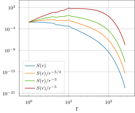 Figure 0
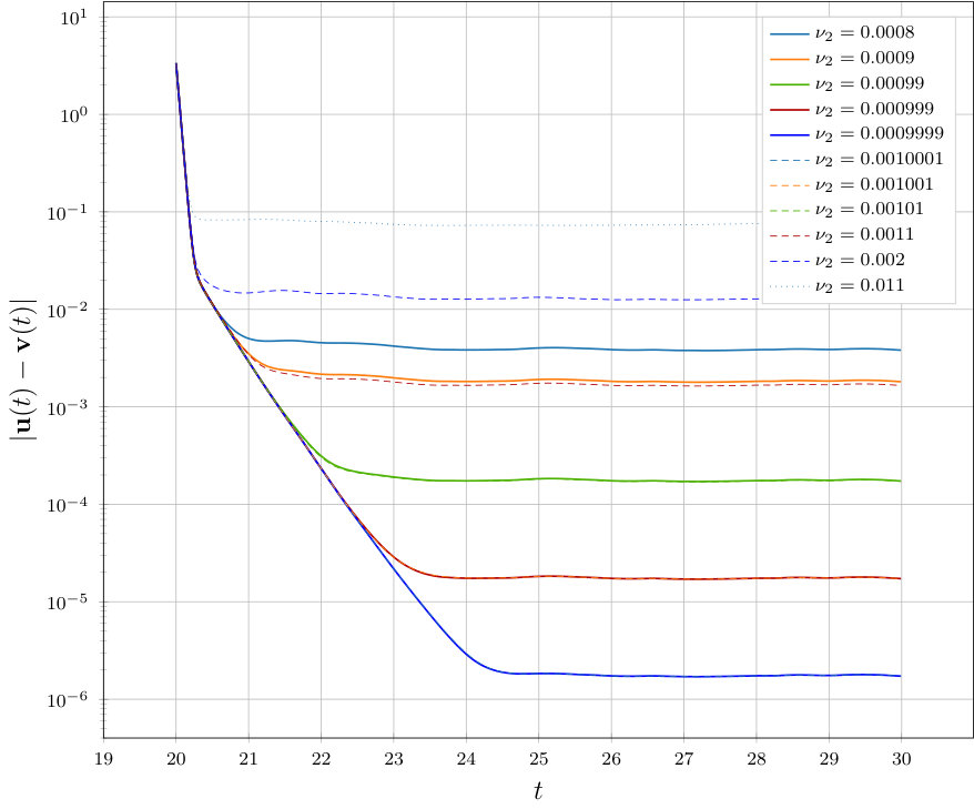 Figure 1
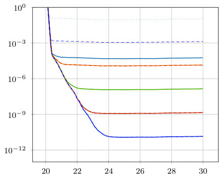 Figure 2
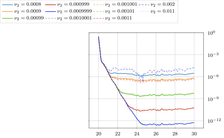 Figure 3
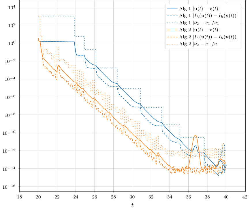 Figure 4
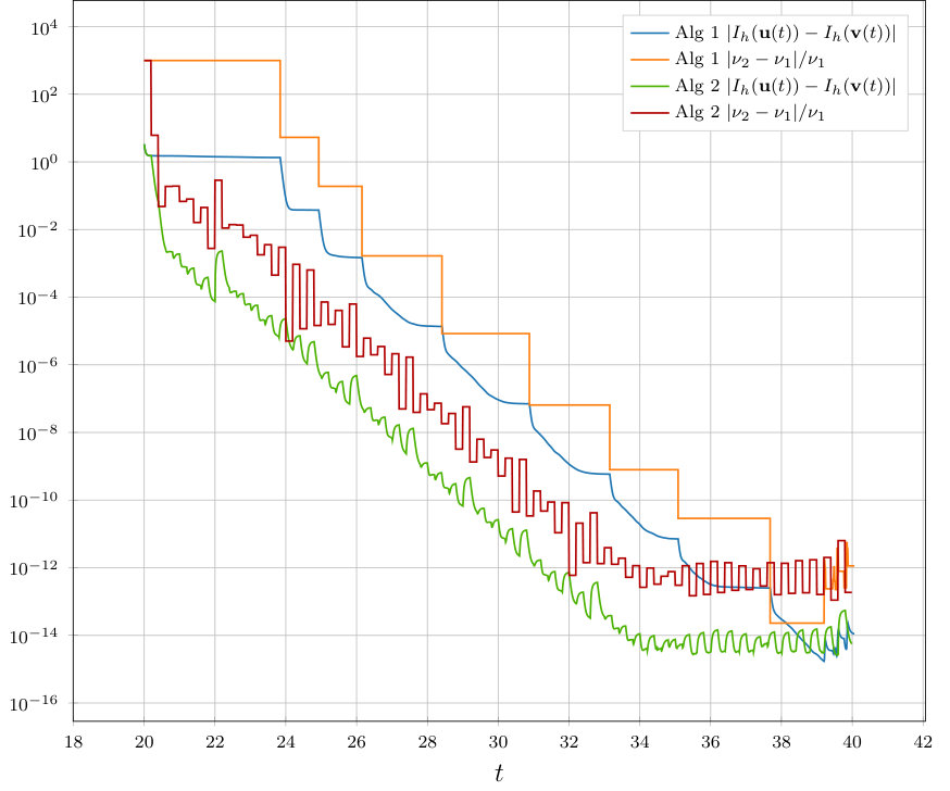 Figure 5
| 0.00080000 | 1.564e-03 | -2.462e-01 | 9.986e-04 | 1.381e-06 | 0.69% |
|---|---|---|---|---|---|
| 0.00090000 | 7.786e-04 | -1.226e-01 | 9.988e-04 | 1.155e-06 | 1.15% |
| 0.00099000 | 7.760e-05 | -1.223e-02 | 9.999e-04 | 1.495e-07 | 1.49% |
| 0.00099900 | 7.762e-06 | -1.222e-03 | 1.000e-03 | 1.423e-08 | 1.42% |
| 0.00099990 | 8.309e-07 | -1.223e-04 | 1.000e-03 | 1.288e-08 | 12.88% |
| 0.00100010 | 8.339e-07 | 1.221e-04 | 1.000e-03 | 1.391e-08 | 13.91% |
| 0.00100100 | 7.765e-06 | 1.222e-03 | 1.000e-03 | 1.328e-08 | 1.33% |
| 0.00101000 | 7.755e-05 | 1.222e-02 | 1.000e-03 | 1.551e-07 | 1.55% |
| 0.00110000 | 7.732e-04 | 1.218e-01 | 1.002e-03 | 1.826e-06 | 1.83% |
| 0.00200000 | 7.570e-03 | 1.183e+00 | 1.031e-03 | 3.121e-05 | 3.12% |
| 0.01100000 | 6.750e-02 | 9.430e+00 | 1.336e-03 | 3.356e-04 | 3.36% |
Peer Reviews
No public reviews on file for this paper yet. If you reviewed it on a platform where reviews are public (OpenReview, ICLR, NeurIPS, ICML), you can paste yours below so the community can read it here.
Videos
No videos yet. Explain this paper in a talk, walkthrough, or lecture? Add one.
Taxonomy
TopicsMeteorological Phenomena and Simulations · Fluid Dynamics and Turbulent Flows · Model Reduction and Neural Networks
Parameter Recovery and Sensitivity Analysis for the 2D Navier-Stokes Equations Via Continuous Data Assimilation
Elizabeth Carlson
Department of Mathematics, University of Nebraska–Lincoln, Lincoln, NE 68588-0130, USA
,
Joshua Hudson
Johns Hopkins University Applied Physics Laboratory, 11100 Johns Hopkins Road, Laurel, MD 20723-6099, USA
and
Adam Larios
Department of Mathematics, University of Nebraska–Lincoln, Lincoln, NE 68588-0130, USA
Abstract.
We study a continuous data assimilation algorithm proposed by Azouani, Olson, and Titi (AOT) in the context of an unknown Reynolds number. We determine the large-time error between the true solution of the 2D Navier-Stokes equations and the assimilated solution due to discrepancy between an approximate Reynolds number and the physical Reynolds number. Additionally, we develop an algorithm that can be run in tandem with the AOT algorithm to recover both the true solution and the Reynolds number (or equivalently the true viscosity) using only spatially discrete velocity measurements. The algorithm we propose involves changing the viscosity mid-simulation. Therefore, we also examine the sensitivity of the equations with respect to the Reynolds number. We prove that a sequence of difference quotients with respect to the Reynolds number converges to the unique solution of the sensitivity equations for both the 2D Navier-Stokes equations and the assimilated equations. We also note that this appears to be the first such rigorous proof of existence and uniqueness to strong or weak solutions to the sensitivity equations for the 2D Navier-Stokes equations (in the natural case of zero initial data), and that they can be obtained as a limit of difference quotients with respect to the Reynolds number.
Key words and phrases:
Parameter Recovery, Sensitivity Analysis, Continuous Data Assimilation, Navier-Stokes Equations, Reynolds Number
MSC 2010 Classification: 34D06, 35A01, 35Q30, 35Q35, 37C50, 76D03
1. Introduction
A major difficulty in performing accurate, practical simulations of dynamical systems is that one typically does not have complete information about the initial state of the system, nor the exact physical parameters of the system, which may be inaccurately measured, or simply unknown. In this paper, we present an algorithm based on data assimilation that addresses both of these difficulties. The term data assimilation refers to a wide class of techniques for incorporating observational data into simulations to increase their accuracy. It is especially relevant for situations in which information about the initial data is sparse. Recently, in a paper by Azouani, Olson, and Titi [4], a new approach to data assimilation, which we refer to as the AOT algorithm, was proposed. This algorithm uses a feedback control term at the PDE level to penalize deviations from the observed data. In the present work, we apply the AOT algorithm in the setting of an unknown diffusion coefficient (e.g., viscosity or ). Moreover, we propose a new algorithm which changes the diffusion coefficient dynamically as the simulation evolves in time, driving the parameter to its true value.
We demonstrate this parameter recovery method for estimating viscosity using the feedback control method of data assimilation proposed in [4], which states that given a dissipative dynamical system (of possibly infinite dimension) of the form
[TABLE]
with missing initial data, we can instead solve the system
[TABLE]
where is a sufficiently large positive relaxation parameter, represents the observational measurements, and is arbitrarily chosen. The function is a straightforward interpolant satisfying particular bounds (stated in the Preliminaries), and is often taken to be modal projection.
Following the analysis of [4] on the 2D incompressible Navier-Stokes equations, analytical bounds on the large time error of with respect to the true solution are shown to be directly dependent upon the difference between our chosen Reynolds number and the true Reynolds number. Computationally, it is observed that the term involving the error of the Reynolds numbers closely matches the error between the solutions and . Due to this fact, we develop a heuristic algorithm for computationally recovering the true viscosity and use this algorithm to simultaneously converge to the true solution .
Since this algorithm introduces a discontinuous change in viscosity during the simulation, we want to ensure that this abrupt change does not lead to the development of shocks in the solution. Thus, we also study the sensitivity of the systems under consideration with respect to perturbation of the diffusion parameter. In particular, we prove that the derivative of solutions with respect to the viscosity is a well-defined object which is bounded in appropriate function spaces; additionally we prove that the corresponding sensitivity equations are globally well-posed in time in an appropriate weak sense and that weak solutions are unique. Sensitivity for partial differential equations has been studied formally in many contexts (see, e.g., [2, 11, 43, 26, 44, 67, 34, 17, 58, 10]). In [64], it was shown formally that the sensitivity equations for the steady-state 2D Navier-Stokes equations are globally well-posed. Additionally, rigorous results on the existence of derivatives of solutions to generic linear and nonlinear differential equations with respect to parameters were proven in [12, 32] via semigroup theory. After the preparation of this manuscript, it also came to our attention that some analysis for the sensitivity equations has been carried out in the slightly more general context of a large eddy simulation (LES) model of the 2D Navier-Stokes equations in an unpublished PhD thesis [57]. In particular, a formal proof of the global existence and uniqueness of the equations was given, based on formal energy estimates. Here, for the convenience of the reader, we provide a fully rigorous proof (although not in the more general LES setting) of the global well-posedness of the sensitivity equations for the 2D Navier-Stokes equations. Moreover, we prove that difference quotients of solutions corresponding to different viscosities converge, in an appropriate sense, to solutions of the sensitivity equations. In this paper, we instead rigorously prove the existence of unique weak solutions with zero initial data to the associated sensitivity equations specifically for the 2D Navier-Stokes equations using the limit of difference quotients corresponding to different viscosities.
Our error estimates in this work are also relevant to the setting of subgrid scale data. In real-world settings, simulations are often underresolved; in particular, it is not always possible to run simulations with the physical Reynolds number (see, e.g., [51, 63, 5], and the references therein). The error estimates we prove in this paper indicate that one may simulate flows using the AOT algorithm with a Reynolds number which is, e.g., smaller than the true Reynolds number, and be assured that deviations from the true solution are controlled (in the and norms) by the difference in the (inverse) Reynolds numbers.
We note that classical data assimilation is largely focused on statistical optimization approaches utilizing the Kalman filter [41] or 3D/4D-Var methods, and variations of these techniques (see, e.g., [16, 42, 49, 52], and the references therein). The AOT algorithm (which is also called continuous data assimilation or CDA in the literature), differs markedly from the Kalman filter approach. Instead of employing statistical tools at the numerical level, AOT data assimilation arises at the PDE level via a feedback-control term which penalizes deviations from interpolations of observable data. This interpolation is a key difference between the AOT method and the so-called nudging or Newtonian relaxation methods introduced in [3, 35], as it allows for significantly more sparse initial data. For an overview of nudging methods, see, e.g., [45] . We mention that a method that shares some features with the AOT algorithm was introduced in [9] in the context of stochastic differential equations. The AOT algorithm and its extensions have been the subject of much recent theoretical work; see, e.g., [1, 6, 7, 8, 14, 21, 22, 23, 24, 25, 28, 29, 30, 33, 36, 37, 38, 39, 46, 54, 55, 59, 61]. Computational trials of the AOT algorithm and its variants were carried out on a wide variety of equations in several recent works, including [18, 31, 48, 50, 19, 53, 47]. We also mention an upcoming work [20], currently a preprint, which explores some similar ideas contained in this paper in the context of continuous data assimilation for the Rayleigh-Bénard convection equations with unknown Prandtl number, although parameter recovery is not explored in that work.
The paper is organized as follows: in Section 2, we describe the mathematical framework for the problems we consider. In Section 3 we consider the AOT data assimilation algorithm and show that with only an approximation of the true viscosity, the reference solution can still be recovered using data assimilation. We analyze the Navier-Stokes equations with periodic boundary conditions, but our techniques can be extended to other boundary conditions and other dissipative systems. In Section 4 we prove rigorous bounds on the sensitivity of the data assimilation approximation on the approximate viscosity used. In Section 5, we provide numerical evidence that illustrates the effectiveness of the algorithm, as well as the practical performance we might expect in a typical flow. In addition, in Section 5.3, motivated by our rigorous results we consider the inverse problem of parameter recovery, and derive an algorithm to recover the true viscosity using data assimilation.
2. Preliminaries
In this section, we state the theorems and other preliminaries needed to solve the incompressible Navier-Stokes equations and the associated modified equations utilizing the AOT algorithm [4]. The statements given in the section without proof are standard, and proofs can be found, e.g., in, e.g., [15, 27, 62, 66, 65]. We consider the incompressible Navier-Stokes equations in dimensionless form on a spatial domain ,
[TABLE]
where is the dimensionless Reynolds number based on the kinematic viscosity , a typical length scale , and typical velocity .
We take the spatial domain, , to be the torus, i.e. , which is an open, bounded, and connected domain with boundary. As is customary, we define the space
[TABLE]
and subsequently the spaces in and in . and are subspaces of and , respectively, and hence are Hilbert spaces with the inner products defined as
[TABLE]
with corresponding norms and . Due to the mean-zero condition, the following Poincaré inequalities hold.
[TABLE]
[TABLE]
Thus, and are equivalent norms on . In 2D, the following Brezis-Gallouet inequality, proven in [13], also holds for all
[TABLE]
We can equivalently consider the Leray projection of the (2.1), where is the orthogonal projection from onto . As in [4], we define the Stokes operator and the bilinear term as the continuous extensions of the operators and defined on as
[TABLE]
and we define the domain of to be . Also note that is a linear self-adjoint and positive definite operator with a compact inverse, so there exists a complete orthonormal set of eigenfunctions in such that , with the eigenvalues strictly positive and monotonically increasing.
We note that the bilinear operator, , has the property
[TABLE]
for all . This implies also satisfies
[TABLE]
for all . Moreover, the following inequalities hold:
[TABLE]
Due to the periodic boundary conditions, it also holds (in 2D) that
[TABLE]
Therefore, for ,
[TABLE]
Additionally, we have the following properties of the bilinear term Lemma 2.1 and 2.3, which we prove using similar strategies as in [62].
Lemma 2.1**.**
Suppose and are uniformly bounded sequences in . Then is uniformly bounded in . Moreover, if and are uniformly bounded in , then is uniformly bounded in .
Proof.
By the definition of the dual norm and (2.3),
[TABLE]
and applying (2.6) we obtain
[TABLE]
Using Hölder’s inequality,
[TABLE]
Hence, since and are uniformly bounded in , it follows that is uniformly bounded in .
Next, suppose and are uniformly bounded sequences in . Then by definition,
[TABLE]
which implies is uniformly bounded in . ∎
Lemma 2.2**.**
Let , and suppose that and strongly in . Suppose also that the sequences and are bounded above uniformly in in . Then in .
Proof.
Take ; then, with
[TABLE]
This implies that
[TABLE]
Since in , in , and the sequences are bounded above uniformly in , we follow the argument in [62] to obtain
[TABLE]
as , and therefore by the density of in , . ∎
Lemma 2.3**.**
If , and strongly in , and and are bounded above uniformly in in , then in .
Proof.
Take ; then
[TABLE]
Applying (2.5), (2.7), and Poincaré’s inequality we obtain
[TABLE]
Applying Agmon’s inequality,
[TABLE]
Since in , in , the sequences are bounded above uniformly in , and is continuous in time, then
[TABLE]
as , and therefore by the density of in , in . ∎
Without loss of generality, we will assume so that . Thus, we may rewrite (2.1) as
[TABLE]
The pressure term can be recovered using de Rham’s theorem [66, 27], a corollary of which is that
[TABLE]
For a given force and some initial data , it is classical that a unique global solution of will exist. However, we don’t expect to know exactly, and so cannot compute from ; rather, we consider the case that measurement data is collected on over the time interval , sufficient for the interpolation operator to construct the interpolation on . From here, we can define a new system, dubbed the data assimilation system, by introducing a feedback control (nudging term) via into (2.11) (or (2.1)), as is done in [4].
We will construct our data assimilation system under the more general case of having only an approximate Reynolds number, :
[TABLE]
Here, is a relaxation parameter, with a kinematic viscosity approximating , and is a linear interpolant satisfying
[TABLE]
From [4], (2.13) has a unique solution given either no-slip Dirichlet or periodic boundary conditions as stated in the following theorem.
Theorem 2.4**.**
Suppose satisfies (2.14) and , where is the constant from (2.14). Then the continuous data assimilation equations (2.13) possess unique strong solutions that satisfy
[TABLE]
for any . Furthermore, this solution is in and depends continuously on the initial data in the norm.
For equations (2.11) and (2.13), we denote the dimensionless Grashof numbers as
[TABLE]
where is the first eigenvalue of the Stokes operator. In 2D, it is classical that (2.1) possesses a unique global strong solution. Furthermore, we have explicit upper bounds on the norms of the solution in and in terms of .
Theorem 2.5**.**
Fix . Suppose that is a solution of , corresponding to the initial value . Then there exists a time which depends on such that for all , it holds that
[TABLE]
In the case of periodic boundary conditions it also holds for all that
[TABLE]
furthermore, if is time-independent then
[TABLE]
To prove our main theoretical results, we will need the following corollary of the statement of the uniform Grönwall lemma proved in [40].
Lemma 2.6** (Generalized Uniform Grönwall Inequality).**
Let be a locally integrable real-valued function defined on , satisfying the following conditions for some :
[TABLE]
[TABLE]
where . Furthermore, let be a real-valued locally integrable function defined on , and let . Suppose that is an absolutely continuous non-negative function on such that
[TABLE]
Then
[TABLE]
where and is chosen sufficiently large so that, for all ,
[TABLE]
and
[TABLE]
We will also make use the following lemma proved in [4].
Lemma 2.7**.**
Let where . Then
[TABLE]
3. Error of Continuous Data Assimilation to Viscosity
We now present our first result. In [4], it was shown for the case , that given a strong solution of (2.1) and an interpolant satisfying (2.14), for sufficiently large and sufficiently small , the corresponding solution of (2.13) will converge in the sense to exponentially fast in time for any , (and convergence in the sense under stronger smoothness assumptions). We extend this result to include the case . In particular, we show that the error decays exponentially in time, down to a level which is controlled by the difference in the (inverse) Reynolds numbers. Moreover, this level goes to zero as . This means that the AOT algorithm for 2D Navier-Stokes can recover the solution approximately even when the true Reynolds number (equivalently, the true viscosity) is unknown, and that the accuracy improves as the approximation of the Reynolds number improves, and with the same order.
Theorem 3.1**.**
Let and be solutions to the systems (2.11) and (2.13), respectively, with initial data , . Suppose , . Let and h\leq\Big{(}\frac{1}{32\pi^{2}c^{2}c_{0}G_{1}^{2}}\frac{\text{Re}_{1}^{2}}{\text{Re}_{2}^{2}}\Big{)}^{1/2}. Then for any such that , and for a.e. , it holds that
[TABLE]
where
[TABLE]
and
[TABLE]
In particular,
[TABLE]
The idea of the proof is similar to the proof of the corresponding result in [4], except that we have an additional term to handle since we allow for the case .
Proof.
We subtract (2.11a) from (2.13a) to obtain
[TABLE]
which can be simplified to
[TABLE]
with initial data given by
[TABLE]
We take the action of (3.1) on , and utilize the Cauchy-Schwarz and Young’s inequalities to obtain
[TABLE]
Using (2.6), (2.14), and Young’s inequality, we obtain
[TABLE]
This implies
[TABLE]
Since, by assumption,
[TABLE]
and
[TABLE]
it follows that
[TABLE]
Hence, we have an inequality of the form (2.21).
Fix such that . Then
[TABLE]
thanks to the assumption . Define
[TABLE]
Choose sufficiently large so that Theorem 2.5 holds and the inequalities (2.22) and (2.23) hold. Then
[TABLE]
and we can apply Lemma 2.6 to conclude that, for a.e. ,
[TABLE]
where . Taking the limit supremum as establishes the result. ∎
We now prove a similar result for the norm of the difference of the solutions, the proof of which closely follows that of [4], although again with an additional term to allow for .
Theorem 3.2**.**
Given the systems (2.11) and (2.13) with periodic boundary conditions, and given , with
[TABLE]
and , then with the following constants:
- •
**
- •
,
- •
,
- •
,
and for any , we obtain
[TABLE]
In particular,
[TABLE]
Proof.
We subtract (2.13a) from (2.11a) to get
[TABLE]
with which, using the identity , can be simplified to
[TABLE]
[TABLE]
Hence,
[TABLE]
By the Brezis-Gallouet inequality,
[TABLE]
Moreover, since by assumption, we obtain
[TABLE]
Using the Cauchy-Schwarz and Young’s inequalities, we find
[TABLE]
Together, the above three inequalities imply that
[TABLE]
Hence,
[TABLE]
Let
[TABLE]
Applying Lemma 2.7 (which is applicable since by Poincaré’s inequality), we obtain
[TABLE]
which can be simplified to
[TABLE]
This implies that
[TABLE]
By (2.20),
[TABLE]
Let . Then
[TABLE]
Young’s inequality implies
[TABLE]
hence,
[TABLE]
Next, we denote and let . Thanks to Theorem 2.5 and the assumption , it follows that
[TABLE]
Clearly, it follows that
[TABLE]
where is defined as in Lemma 2.6.
Choose sufficiently large so that Theorem 2.5 holds and the inequalities (2.22) and (2.23) hold. Then, we can apply Lemma 2.6 to obtain, for a.e. ,
[TABLE]
where as defined in Lemma 2.6. Taking the limit supremum as establishes the result. ∎
Sensitivity for partial differential equations has been studied formally in many contexts (see, e.g., [2, 10, 12, 17, 26, 32, 34, 43, 44, 56, 57, 58, 60, 64, 67].
4. Sensitivity
In this section, we analyze the sensitivity of to the Reynolds number by considering individually the sensitivity of and to the Reynolds number. We wish to consider taking a derivative of equations (2.11a) and (2.13a) with respect to the Reynolds number. This has been done formally in many works on sensitivity (see, e.g., [2, 10, 11, 17, 26, 34, 43, 44, 57, 58, 67]), yielding what are known as the sensitivity equations. However, to the best of our knowledge, a rigorous treatment has yet to appear in the literature. Therefore, we provide a rigorous justification here of the existence and uniqueness of weak and strong solutions to the sensitivity equations in the case of zero initial data, which is the natural data for the sensitivity equation, as discussed below. Moreover, we prove that these solutions can be realized as limits of difference quotients of Navier-Stokes solutions with respect to different Reynolds numbers. Indeed, this is the method of our existence proofs, rather than using, e.g., Galerkin methods, fixed-point methods, etc. Proofs using limits of difference quotients have appeared in the literature before, such as in standard proofs of elliptic regularity, the corresponding result for the Stokes equations, etc. However, in the present context (i.e., the time-dependent sensitivity equations for 2D Navier-Stokes), we believe such a proof strategy is novel.
Working formally for a moment, we take the derivative of (2.11a) with respect to Re, and denote (again, formally) and , to obtain
[TABLE]
These are known as the sensitivity equations for the Navier-Stokes equations. Similarly, denoting and , we formally obtain
[TABLE]
Below, we prove some well-posedness results for these systems in the case of zero initial data. We begin by defining what we mean by solutions.
Remark 4.1*.*
We note that the sensitivity equations are a model for the evolution of the instantaneous change in a solution with respect to changes in the (inverse) Reynolds number. Therefore, the natural initial condition to consider is the case of identically-zero initial data. Indeed, if the initial data for the sensitivity equations is not identically zero, this would correspond to the case where the initial data for the Navier-Stokes equations depends on the viscosity, which is not typical of most mathematical treatments of the Navier-Stokes equations. Thus, although we define weak solutions for general initial data, we only prove their existence for initial data which is identically zero. Existence for general initial data can be proved using, e.g., Galerkin methods. However, since our main focus is not on existence, but on showing the solutions can be realized as limits of a (sub)sequence of difference quotients, and moreover since the initial data is naturally taken to be zero in this setting, we use the difference quotient method instead.
Definition 4.2**.**
Let . Let be a weak solution to (2.1) with initial data and forcing . A weak solution of (4.1) is an element satisfying and
[TABLE]
for a.e. , for all , and initial data , satisfied in the sense of .
If, in addition, , , , and is a strong solution to (2.1), then we define a strong solution of (4.1) to be a weak solution such that and , satisfying (4.3) for a.e. and for all .
For the reasons discussed in Remark 4.6 below, we only give a definition of strong solutions for the assimilation equations.
Definition 4.3**.**
Let . Let be a strong solution to (2.13) with initial data and forcing . A strong solution of (4.2) is an element that satisfies
[TABLE]
this equation for a.e. and for all , where and initial data .
Before we prove the existence and uniqueness of solutions with zero initial data to these equations, we first consider equations for the difference quotients. Note that, since these are simple arithmetic operations on the Navier-Stokes equations, the manipulations can be performed rigorously, not just formally. To this end, let be a solution to (2.1) with Reynolds number and be a solution to (2.1) with Reynolds number with the same initial data. We take the difference of the two versions of (2.1), each with Reynolds numbers and . We then divide by the difference in (inverse) Reynolds numbers, yielding the system
[TABLE]
where and . As defined, is a strong solution to (4.4), and note that . Additionally, and . However, we need to establish that is the unique solution to (4.4), which is the content of Lemma 4.4 below.
Lemma 4.4**.**
Let be given, and let , be strong solutions to (2.13), with Reynolds numbers and , respectively. There exists one and only one solution to (4.4) that lies in , i.e. for all ,
[TABLE]
where .
Next, we consider difference quotients for the assimilation system (2.13). Let be the solution to (2.13) with Reynolds number and be the solution to (2.13) with Reynolds number . Subtracting the two equations and dividing by the difference in the (inverse) Reynolds numbers yields the system (4.5),
[TABLE]
where and . As defined, is a strong solution to (4.5), and note that . Additionally, and .
Lemma 4.5**.**
Let be given ,and let , be strong solutions to (2.13), with Reynolds numbers and , respectively. There exists a unique strong solution to (4.5) that lies in , in the sense that for all ,
[TABLE]
where .
Remark 4.6*.*
The proofs of the above two lemmata are very similar; hence, we only present the proof of Lemma 4.5. Moreover, we also note that in the case , the proof of Lemma 4.4 holds mutatis mutandis in the case where , are only assumed to be weak solutions to the 2D Navier-Stokes equations, and then one obtains uniqueness of weak solutions to (4.4) in the class . However, in the case , the notion of weak solutions for the assimilation equations (2.13) has not been established in the literature for general interpolants , and therefore we assume that the solutions and are strong solutions to (2.13), and prove the uniqueness of strong solutions to (4.4).
Proof.
Suppose there exist two solutions and . We consider the difference of the equations
[TABLE]
and
[TABLE]
which, defining , yields
[TABLE]
with . So, must be a solution to the above equation. Taking the inner product with ,
[TABLE]
which implies, applying the triangle inequality and Poisson’s inequality to the interpolant term as in [4],
[TABLE]
Thus,
[TABLE]
and Grönwall’s inequality implies
[TABLE]
But , and thus implies that . Hence, solutions to (4.5) are unique. ∎
Since systems (4.4) and (4.5) have unique strong solutions for every , we want to show that, as , the solutions to these equations converge to the unique strong solutions of the respective equations (in the sense of Definitions 4.2 and 4.3) of the formal sensitivity equations (4.1) and (4.2) with [math] initial data. We additionally prove that weak solutions exist for the sensitivity equations (4.1) with [math] initial data.
Theorem 4.7**.**
Let be a sequence such that as . Let
- •
* be a solution to (2.1) with Reynolds number , forcing , and initial data ;*
- •
* solve (2.1) with viscosity , forcing , and initial data ;*
- •
* be a sequence of strong solutions to (4.4) with .*
Then there is a subsequence of that converges in to a unique weak solution of (4.1) with [math] initial data for any .
Proof.
Let be given. Let sufficiently large such that for all , . Then, we can follow the proof of strong solutions for (2.1) as in, e.g., [15, 27, 62, 66], to obtain bounds on for in the appropriate spaces that are independent of :
[TABLE]
and
[TABLE]
Note that since all bounded functions are locally integrable. Hence there is a subsequence that is relabeled in for some function . Continuing to follow the proof of strong solutions for (2.1) as in e.g. [15, 27, 62, 66], we note that is uniformly bounded in in . Hence, we can find a subsequence which we relabel such that
[TABLE]
Indeed, satisfies (2.1) with corresponding Reynolds number and thus, by uniqueness and the fact that in , . Due to Poincaré’s inequality, we also obtain that in .
Let be the strong solution to (4.4) with . Taking the action of (4.4) on and using Hölder’s, the bilinear inequalities, and Young’s inequality twice, we obtain
[TABLE]
giving
[TABLE]
Dropping the second term on the left hand side, we obtain
[TABLE]
Taking the integral with respect to time on and applying Grönwall’s inequality, then for a.e. ,
[TABLE]
Since , then is bounded above uniformly in .
Next, refraining from dropping the second term on the left hand side of (4.13), we estimate
[TABLE]
Rewriting, we obtain
[TABLE]
Thus, is bounded above uniformly in with respect to . Hence, by the Banach-Alaoglu Theorem, there exists a subsequence, relabeled as , such that
[TABLE]
Using (4.14), note that all uniform bounds in on the terms in (4.4) in are obtained in a similar manner to the proof of weak solutions for (2.1) except for the term . However, by Lemma 2.1,
[TABLE]
and due to the following bounds on (which can be found in [15, 27, 62, 66], etc.) and the fact that ,
[TABLE]
and
[TABLE]
and thus is bounded above uniformly in independent of . Hence, independent of , is bounded above uniformly in and by the Banach-Alaoglu Theorem a subsequence converges weakly to in . Thus, by the Aubin Compactness Theorem, strongly in . Hence, weak continuity in follows due to the bounds on each of the terms above. Using these facts, we have weak- convergence in of all but the bilinear terms in the standard sense. Weak- convergence of the bilinear terms holds due to Lemma 2.2, yielding in . Additionally since strongly in , we can apply Lemma 2.2 again to obtain that . Thus, satisfies
[TABLE]
in . The initial condition is satisfied by construction. To prove uniqueness, suppose that there exist two weak solutions and . We consider the difference of the equations
[TABLE]
and
[TABLE]
which, defining , yields
[TABLE]
with . So, must be a weak solution to the above equation. Taking the action on and applying the Lions-Magenes Lemma,
[TABLE]
which implies
[TABLE]
Dropping the second term, we obtain
[TABLE]
and Grönwall’s inequality implies that, for a.e. ,
[TABLE]
Since we know the \text{exp}\Big{(}\int_{0}^{T}\frac{c^{2}}{2\text{Re}_{1}^{-1}}\|\mathbf{u}_{1}\|^{2}dt\Big{)}<\infty for all and , we have that , which implies that . Hence, weak solutions to (4.4) are unique. ∎
Theorem 4.8**.**
Let be a sequence such that as . Let
- •
* be the solution to (2.1) with Reynolds number , forcing , and initial data ;*
- •
* solve (2.1) with viscosity , forcing , and initial data *
- •
* be a sequence of strong solutions to (4.4) with .*
Then there is a subsequence of that converges in to a unique strong solution of (4.1) with [math] initial data.
Proof.
Let be given, and let be large enough that implies . Then by the argument in Theorem 4.7, we can obtain a subsequence which we relabel such that in .
Consider to be the strong solution to (4.4) with Reynolds number . Taking a justified inner product of (4.4) with ,
[TABLE]
Applying Young’s inequality, we obtain
[TABLE]
Applying (2.5) to the second bilinear term,
[TABLE]
and applying (2.7) to the first bilinear term,
[TABLE]
which can be rewritten as
[TABLE]
Integrating on both sides in time, with ,
[TABLE]
Dropping the second term on the left hand side, we apply Grönwall’s inequality to obtain
[TABLE]
where . Since
[TABLE]
as proven in, e.g., [15, 62, 27, 66], then
[TABLE]
This implies that and is uniformly bounded in this space.
Additionally, considering again the inequality
[TABLE]
we set , drop the first term on the left hand side, and bound the Reynolds number above to obtain
[TABLE]
By the fact that is bounded above in as demonstrated in Theorem 4.7 and the result that is bounded above uniformly in , we also have that is bounded above uniformly in . Since is bounded above uniformly in in both and , then we can conclude that there exists a subsequence, which we relabel as , such that
[TABLE]
Using (4.15), note that all uniform bounds in on the terms in (4.4) in are obtained in a similar manner to the proof of strong solutions for the (2.1) and are independent of except for the bilinear terms. The bilinear terms are bounded uniformly in with respect to , due to Lemma 2.1. Hence, is bounded above uniformly in in . Thus, as in, e.g., [62, 15, 27, 66],
[TABLE]
Hence, by the Aubin Compactness Theorem, strongly in . As in, e.g., [62, 66, 27, 15], . Using these facts, we have weak convergence in for all except the bilinear terms in the standard sense. Weak convergence of the bilinear terms holds due to Lemma 2.3. Hence, satisfies
[TABLE]
in .
The initial condition is also satisfied by construction. Uniqueness holds due to the results in Theorem 4.7. ∎
Theorem 4.9**.**
Let be a sequence such that as . Choose and such that . Let
- •
* be the solution to (2.13) with Reynolds number , forcing , and initial data ;*
- •
* solve (2.13) with viscosity , forcing , and initial data ;*
- •
* be a sequence of strong solutions to (4.5) with .*
*Then there is a subsequence of that converges in to a unique solution of (4.2) with [math] initial data. *
Proof.
Let . Note that since for for some sufficiently large , we can follow the proof of strong solutions for (2.13) in [4] to obtain bounds on in the appropriate spaces that are independent of . First, we note that [4] quickly proves since . However, since is bounded above uniformly in (see the proof of Theorem 4.7), we have that for some independent of . Thus, we have the following bounds from [4] bounded above uniformly in :
[TABLE]
[TABLE]
[TABLE]
where
[TABLE]
which is bounded above uniformly in due to (4.16) and (4.17), and
[TABLE]
which is bounded above uniformly in due to (4.16), (4.17), (4.18). Hence, we will obtain a subsequence that is relabeled in for some function . Indeed, we see that by identical arguments presented in Theorem 4.7, . Also due to Poincaré’s inequality, we obtain that in .
Let be a sequence of solutions to (4.5). We consider the Leray projection of (4.5):
[TABLE]
The existence proof for (4.2) closely follows the proof of Theorem 4.8, with some modifications on the bounds of which we show below. Taking the inner product with and proceeding as in the proof of Theorem 4.8, we obtain
[TABLE]
We slightly modify the inequalities obtained in [4] for the interpolant term,
[TABLE]
Also,
[TABLE]
Using these inequalities in (4.19):
[TABLE]
Following identical arguments as in Theorem 4.8 with
[TABLE]
along with the fact that is bounded uniformly in in , we obtain a subsequence relabeled in . Indeed, let ; then
[TABLE]
Additionally, since we now have that in , then in and we conclude is a strong solution in the sense of Definition 4.3.
To show that the solutions are unique, we consider the difference of the equations
[TABLE]
and
[TABLE]
which, defining , yields
[TABLE]
with . So, must be a solution to the above equation. Taking the action on and applying the Lions-Magenes Lemma,
[TABLE]
which implies that
[TABLE]
Thus,
[TABLE]
and Grönwall’s inequality implies, for a.e. ,
[TABLE]
But , and thus implies that . Hence, solutions to (4.5) are unique. ∎
5. Numerical Results
In the previous sections, we showed that the data assimilation algorithm (2.13) can still perform well even when there is error in the viscosity parameter, provided that is large and is small. However, for large values of the Grashof number satisfying the requirements of the rigorous estimates would require prohibitively small values of . Fortunately, in practice the requirements on and need not be strict when is known, and in fact we would expect the algorithm to perform well with very modest values for and (see [31]).
In addition, the complexity of small viscosity flows requires more computational resources to accurately simulate, but our results indicate that if one has (coarse) measurement data collected on such a flow continuously over a time interval it may be possible to construct an accurate computational simulation of the flow over the same time interval, using a much larger value for the viscosity, saving computational resources. Note that one would still need to use the true, smaller viscosity in our simulations after time to accurately predict the behavior of the flow, because we have no data after time . In Section 5.2 we test the effectiveness of such an approach numerically.
Lastly, although our primary purpose in the preceding section was to obtain an upper bound on the data assimilation error, in doing so we have obtained a lower bound on the viscosity error, , in terms of the resulting data assimilation error. In light of this fact, in Section 5.3 we construct a rudimentary algorithm to estimate the value of the true (but unknown) viscosity, , using data collected on the flow, , and the solution of the data assimilation algorithm, . We then test the algorithm numerically.
5.1. Computational Setting
All of the following computations were performed on the supercomputer Karst at Indiana University, using dedalus, an open source pseudo-spectral python package, available at http://dedalus-project.org. A computational resolution was used, with a 3/2 dealiasing factor. A simple explicit/implicit time stepping scheme was used for each simulation, where the linear terms were handled implicitly, and the nonlinear terms explicitly. The spatial domain we consider is , so . For simplicity, and to limit our assumptions about prior knowledge of the reference solution, we will take the typical velocity to be , so that and in our calculations in the previous sections. With this choice of typical velocity, the Reynolds numbers we define do not characterize the resulting flows in the typical way, so we will instead use the viscosities.
5.1.1. Reference Solution
We take our reference solution to be the solution, , of (2.1) with
[TABLE]
and
[TABLE]
and with the initial condition . Each is normally distributed, and scaled so that .
We do not have a closed form solution for so instead we approximate it numerically by solving (2.1) computationally over the time interval . We call the computational approximation we obtain , and denote its Fourier transform by . So, for all ,
[TABLE]
Figure 5.1 shows the spectrum of over the time interval , where we define the spectrum, , by
[TABLE]
5.1.2. Data Assimilation Parameters
In the following numerical experiments, we only consider the case that is the projection onto the low modes, i.e.
[TABLE]
We used a spectral method to compute , so we can readily construct . In a practical situation, would be given to us and we would have no knowledge of ; instead, we use to compute , with the expectation that for all after a time . In Section 5.2 we simulate this situation by computing and comparing it to .
Before we can compute , we will need to choose values for and . The rigorous estimates we have obtained thus far are sufficient conditions, and do not determine the most efficient values of and in practice. Specifically, for the reference solution we have computed, , so to satisfy the requirements of Theorem 3.1, we would need and . To compute with , in addition to requiring a large amount of data in practice, would require we increase the computational resolution at least to . Fortunately, the algorithm works with much less data, and with much smaller .
For simplicity, we will only consider
[TABLE]
5.2. Subgrid Simulations
We are now ready to test the performance of the data assimilation algorithm when . We compute the solutions of (2.13) corresponding to several values of , with percentage error, , ranging from to . Each solution is computed over the time interval with the initial condition . Starting the data assimilation simulation at time is sufficient in this case to ensure that is past a transient (and so is approximating a physical flow), and will be nontrivial at (and therefore differs from at the start of the simulation).
Figure 5.2 shows the resulting error we observe for each simulation when we compare to over the same time interval. We see that for each simulation, after a transient period of fast convergence, the error decreases exponentially at a nearly constant rate before reaching a minimum value. Also, the rates of convergence are the same for each simulation.
5.3. Parameter Recovery
We can see in Figure 5.2 that the error in the viscosity value is directly correlated with the minimum error achieved by the corresponding data assimilation solution. This observation motivates the following: given the data , we can compute and use the minimum error we observe to estimate the true viscosity, .
Although is sufficient to compute , we would need to have to compute . Fortunately, we see that and are also correlated, as can be seen in Figure 5.3.
With this in mind, we will now study this correlation, so that, once it’s nature is established, we can use it to develop an algorithm to estimate .
5.3.1. A posteriori Error Estimate
The result in Theorem 3.1, in addition to being in terms of the true error (as opposed to the error of only the interpolations of and ), establishes bounds for the data assimilation error in terms of the Grashof number. We are now considering a situation where we have access to , and so would like to obtain a sharper estimate on the error by allowing it to be in terms of instead of .
As in the proof of Theorem 3.1, let . Using the facts that
[TABLE]
and
[TABLE]
we can replace (3.1) with
[TABLE]
Now, we apply to both sides of this equation and obtain
[TABLE]
Next, we take the inner product with and use the fact that
[TABLE]
The result, after rearranging terms, is
[TABLE]
We have observed in each of our simulations that there is a time at which the error reaches a minimum value and thereafter remains constant; then , and the above equation reduces to
[TABLE]
Note that all of the terms on the left hand side of (5.3) except are explicitly computable from data observations. However, on the right hand side, one would need to compute and . Also, although in the periodic setting, commutes with the projection onto the low Fourier modes, might not commute with other types of interpolation operators , in which case one could not compute exactly from the observations .
However, we note that in terms of units, each of the terms in (5.3) decreases quadratically with as (with the exception of ), but we control and have chosen large enough that dominates the terms on the right hand side, as can be seen in Figure 5.3. Therefore, we propose an approximation formed by dropping these terms from the equation, and solving (approximately) for , thereby obtaining
[TABLE]
Since each time on the right-hand side now depends only on given or observable quantitesm, This approximation motivates an iterative scheme for recovering the viscosity. We therefore test (5.4) as a means of recovering , using the data from our simulations. We obtain the approximation iteratively, using (5.4) for each of the simulations performed in Section 5.2 at time , and compare to . The results are shown in Table 5.3.1. In each case, (5.4) produces a much better approximation of the true , showing at least an improvement.
The reference list from the paper itself. Each links out to its DOI / PubMed record.
- 1[1] D. A. Albanez, H. J. Nussenzveig Lopes, and E. S. Titi. Continuous data assimilation for the three-dimensional Navier–Stokes- α 𝛼 \alpha model. Asymptotic Anal. , 97(1-2):139–164, 2016.
- 2[2] K. Anderson, J. C. Newman, D. L. Whitfield, and E. J. Nielsen. Sensitivity analysis for Navier–Stokes equations on unstructured meshes using complex variables. AIAA Journal , 39, 11 1999.
- 3[3] R. A. Anthes. Data assimilation and initialization of hurricane prediction models. J. Atmos. Sci. , 31(3):702–719, 1974.
- 4[4] A. Azouani, E. Olson, and E. S. Titi. Continuous data assimilation using general interpolant observables. J. Nonlinear Sci. , 24(2):277–304, 2014.
- 5[5] L. C. Berselli, T. Iliescu, and W. J. Layton. Mathematics of Large Eddy Simulation of Turbulent Flows . Scientific Computation. Springer-Verlag, Berlin, 2006.
- 6[6] H. Bessaih, E. Olson, and E. S. Titi. Continuous data assimilation with stochastically noisy data. Nonlinearity , 28(3):729–753, 2015.
- 7[7] A. Biswas, C. Foias, C. F. Mondaini, and E. S. Titi. Downscaling data assimilation algorithm with applications to statistical solutions of the Navier–Stokes equations. In Annales de l’Institut Henri Poincaré C, Analyse non linéaire . Elsevier, 2018.
- 8[8] A. Biswas and V. R. Martinez. Higher-order synchronization for a data assimilation algorithm for the 2D Navier–Stokes equations. Nonlinear Anal. Real World Appl. , 35:132–157, 2017.