Asymptotic analysis of Dotsenko-Fateev integrals
Jonatan Lenells, Fredrik Viklund

TL;DR
This paper introduces a new method for asymptotic analysis of Dotsenko-Fateev integrals, which are important in conformal field theory and SLE processes, providing useful estimates for related martingale observables.
Contribution
It develops a novel approach to evaluate asymptotics of Dotsenko-Fateev integrals, generalizing classical hypergeometric functions and aiding in SLE martingale analysis.
Findings
Established estimates for Dotsenko-Fateev integrals
Enhanced understanding of their asymptotic behavior
Applications to martingale observables in SLE
Abstract
We develop a method for evaluating asymptotics of certain contour integrals that appear in Conformal Field Theory under the name of Dotsenko-Fateev integrals and which are natural generalizations of the classical hypergeometric functions. We illustrate the method by establishing a number of estimates that are useful in the context of martingale observables for multiple Schramm-Loewner evolution processes.
Click any figure to enlarge with its caption.
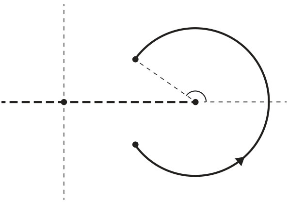 Figure 1
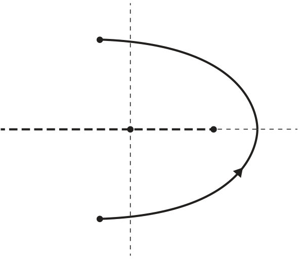 Figure 2
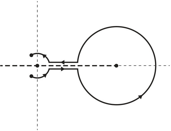 Figure 3
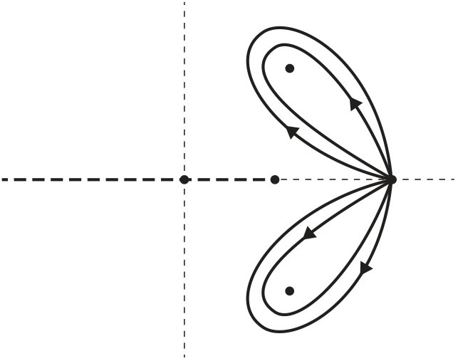 Figure 4
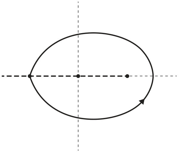 Figure 5
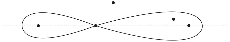 Figure 6
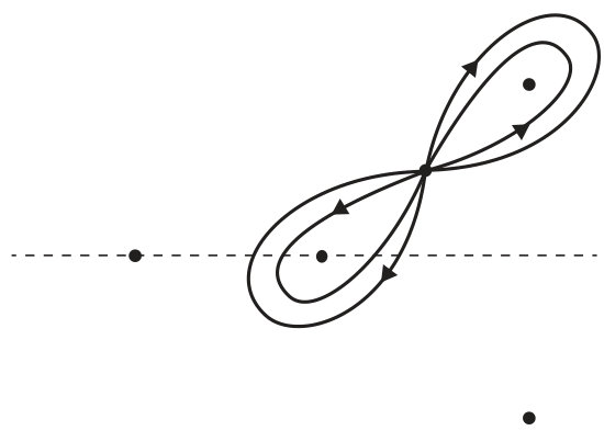 Figure 7
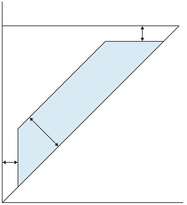 Figure 8
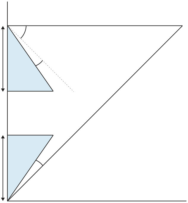 Figure 9
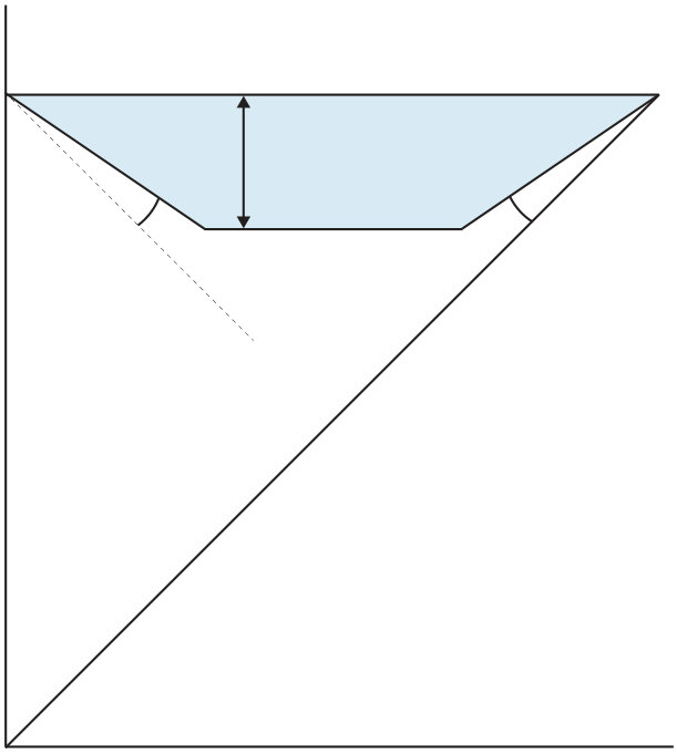 Figure 10
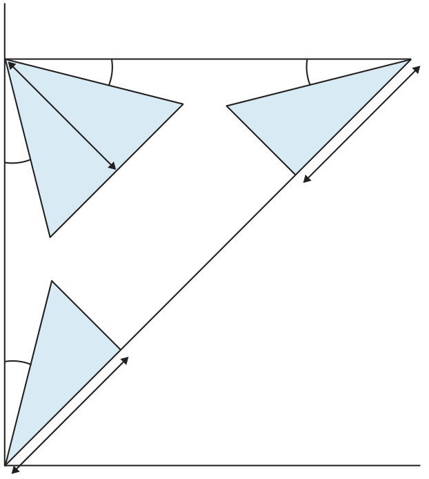 Figure 11
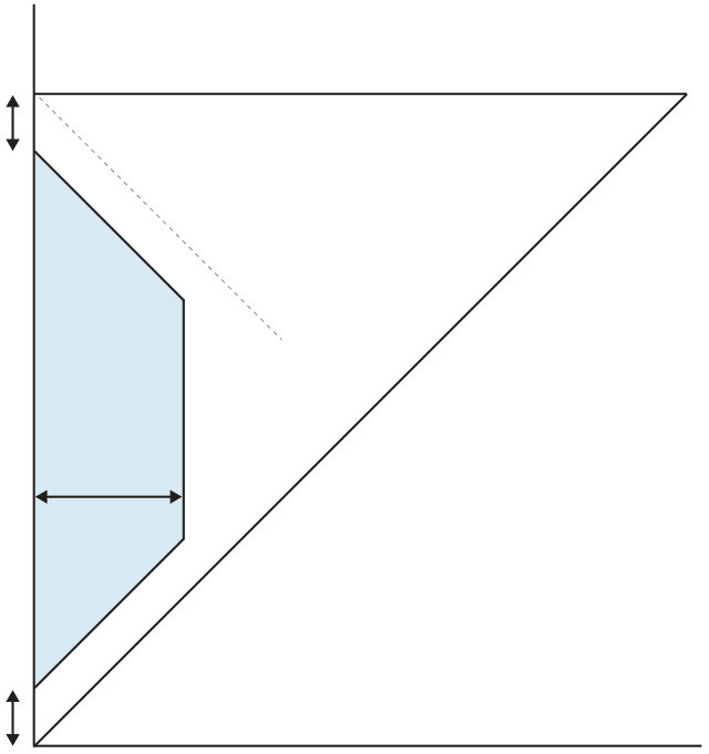 Figure 12
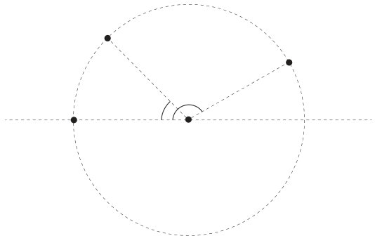 Figure 13
Peer Reviews
No public reviews on file for this paper yet. If you reviewed it on a platform where reviews are public (OpenReview, ICLR, NeurIPS, ICML), you can paste yours below so the community can read it here.
Videos
No videos yet. Explain this paper in a talk, walkthrough, or lecture? Add one.
Asymptotic analysis of Dotsenko-Fateev integrals
Jonatan Lenells and Fredrik Viklund
Department of Mathematics, KTH Royal Institute of Technology,
100 44 Stockholm, Sweden.
[email protected], [email protected]
Abstract.
We develop a method for evaluating asymptotics of certain contour integrals that appear in Conformal Field Theory under the name of Dotsenko-Fateev integrals and which are natural generalizations of the classical hypergeometric functions. We illustrate the method by establishing a number of estimates that are useful in the context of martingale observables for multiple Schramm-Loewner evolution processes.
AMS Subject Classification (2010): 30E15, 33C70, 81T40.
Keywords: Integral asymptotics, conformal field theory, Schramm-Loewner evolution.
Contents
1. Introduction
In this paper, we will be interested in integrals of the form
[TABLE]
where is an integer, is a set of exponents, is a finite collection of points, and the Pochhammer integration contour encloses two of these points, say and . More precisely, the Pochhammer contour in (1.1) begins at the base point , encircles once in the positive (counterclockwise) direction, returns to , encircles once in the positive direction, returns to , encircles once in the negative direction, returns to , and finally encircles once in the negative direction before returning to , see Figure 1. The remaining points are assumed to lie exterior to the contour and the powers in the integrand are assumed to take their principal values at the starting point and are then analytically continued along the contour.
By employing what is sometimes called the screening method, Dotsenko and Fateev obtained representations of correlation functions in Conformal Field Theory (CFT) in terms of such integrals [3, 4] (see also [2]). Integrals of the form (1.1) are therefore often referred to as Dotsenko-Fateev integrals. Various aspects of such integrals and related special functions have been studied in a number of places, e.g., [7, 8]. For and , the integral (1.1) can be expressed in terms of Gamma functions and the classical hypergeometric function , respectively. In the case of , a comparison with the representation of Appell’s function as an Euler integral (cf. [7]) shows that (1.1) can be viewed as an analytic continuation of Appell’s function. We also mention [5, 9, 10] which discuss related questions in the context of the Schramm-Loewner Evolution (SLE).
The basic problem we are interested in here is how to compute the asymptotics of the integral (1.1) as one (or several) of the points , , approaches or . The computation of such asymptotics presents difficulties, because if the point , , approaches , say, then the contour gets squeezed between and which, in general, gives rise to a singular behavior. For , the relevant asymptotics can be obtained from well-known identities and expansions of hypergeometric functions. However, for , the analysis is more intricate.
In this paper, we propose a method which makes it possible to compute the asymptotics of (1.1) to all orders for any as one (or many) of the points , , approaches or . The obtained expansions are power series in the relevant small quantities with coefficients explicitly given in terms of Gamma functions and integrals of the form (1.1) of a lower order . In the case of , it is conceivable that the asymptotic formulas we derive can be obtained also from known properties of Appell’s function. However, as far as we are aware, formulas of this type have not appeared in the literature even in this simplest case.
By applying a linear fractional transformation, we may assume that and in (1.1); this yields an expression of the form
[TABLE]
For simplicity, we will present the results in this paper for the class of integrals corresponding to . Although the proposed method works for arbitrary values of and an arbitrary number of merging points, its application involves a large number of steps when is large (the number of steps typically grows like , because, roughly speaking, each time two points merge one of the series contributing to the asymptotics splits into two).
1.1. Brief description of method
Let denote the integral in (1.2) for , that is, is defined for by
[TABLE]
where is a base point, are real exponents, and are assumed to lie outside the contour. In order to make single-valued, we have restricted the domain of definition in (1.3) to . We will assume that are not integers, because otherwise the integral in (1.3) vanishes identically or can be computed by a residue calculation. Note that can be analytically continued to a multiple-valued analytic function of . Our goal is to compute the asymptotic behavior of to all orders as one or both of the points and approach [math] or .
The basic idea is the following: If we want to consider the limit say, then we rewrite as a sum of two terms (see equation (4.13)). One term which is defined by the same integral as except that is now assumed to lie inside the contour in the same component as [math] (see equation (4.11)), and a second term which is defined by a similar expression but with the Pochhammer contour enclosing instead of (see (4.12) and (4.15)). The asymptotics of both of these terms can easily be computed to all orders by simply replacing the factors in the integrands by their asymptotic expansions as such as
[TABLE]
We emphasize that it is, in general, not possible to compute the asymptotics of as by substituting the expansion (1.4) directly into (1.3). Indeed, such a procedure gives the correct contribution from the first term, but completely ignores the contribution from the second term.
1.2. Two examples
Our initial motivation for studying asymptotics of integrals of the form (1.1) was that they appear naturally when constructing observables for multiple SLE curves via the screening method within CFT. Thus, in the second part of the paper, in order to illustrate our method, we consider two concrete examples of such observables where integrals of the form (1.1) are important. By applying the techniques developed in the first part of the paper, we are able to derive asymptotic estimates for the integrals in these examples. The estimates we establish are used in the derivation of the Green’s function and Schramm’s formula for multiple SLE presented in [11]. We expect similar asymptotic estimates to be needed also in the context of other SLE observables derived via the screening method.
1.3. Organization of the paper
In Section 2, we present four different examples of asymptotic expansions to all orders which can be derived by our method. Before turning to the full description of the method and the proofs of the above expansions in Section 4, we consider the hypergeometric case of in Section 3 as motivation. The two examples from SLE theory are introduced in Section 5. In Section 6, we derive the estimates relevant for the first example corresponding to the Green’s function. In Section 7, we derive the estimates relevant for the second example corresponding to Schramm’s formula.
2. Four asymptotic theorems
The purpose of this paper is to propose a method which makes it possible to compute the asymptotics of (1.2) as one (or several) of the points , , approaches [math] or . There are clearly many different cases to consider depending on the value of , on the number of points involved in the limiting process, and on whether each approaches [math] or . For the sake of presentation, we have chosen to discuss four cases in detail. The presented cases all have and correspond to the following limits: (a) , (b) , (c) and , and (d) and . These four cases, which are treated one by one in Theorem 2.1-2.4, illustrate the different situations that may arise and it will be clear from the analysis of these cases how to apply the method also in other cases.
2.1. Notation
We let , , and denote the integral given in (1.2) for , , and , respectively. That is, is defined by (1.3), is defined by
[TABLE]
where is assumed to lie outside the contour, and is defined by
[TABLE]
The Pochhammer integration contour in (2.1) begins at the base point , encircles the point [math] once in the positive (counterclockwise) direction, returns to , encircles once in the positive direction, returns to , and so on. The point lies exterior to all loops; the factors in the integrand take their principal values at the starting point and are then analytically continued along the contour. A similar interpretation of Pochhammer contours applies to the definition (1.3) of and elsewhere. Throughout the paper we adopt the convention that unless stated otherwise, the principal branch is used for all complex powers and logarithms, i.e., with . For , we define by
[TABLE]
2.2. Asymptotic theorems
We can now state the asymptotic results. The proofs are given in Section 4.
Theorem 2.1** (Asymptotics as ).**
Let be such that . Then satisfies the following asymptotic expansion to all orders as with :
[TABLE]
where the coefficients , , are given by
[TABLE]
Theorem 2.2** (Asymptotics as ).**
Let be such that . Then satisfies the following asymptotic expansion to all orders as with :
[TABLE]
where the coefficients , , are given by
[TABLE]
Theorem 2.3** (Asymptotics as and with ).**
Let be such that . Then satisfies the following asymptotic expansion to all orders as and with such that for some :
[TABLE]
where the coefficients , , are given by
[TABLE]
Theorem 2.4** (Asymptotics as and ).**
Let be such that . Then satisfies the following asymptotic expansion to all orders as and with :
[TABLE]
where the coefficients , , are given by
[TABLE]
Remark 2.5**.**
For definiteness, we have stated Theorem 2.3 under the assumption that . It will be clear from the full description of the method in Section 4 that the case can be treated similarly. The case can also be handled by similar steps, but in this case the coefficients depend on the quotient . In fact, a slight modification of the proof of Theorem 2.3 yields the following result (see Remark 4.4): If satisfy and , then satisfies the following asymptotic expansion to all orders as and with such that and for some :
[TABLE]
where and the coefficients , , are given by
[TABLE]
Here is defined by the same formula (2.1) as except that is assumed to lie inside the contour in the same component as [math].
Remark 2.6**.**
The function defined in (2.2) can be expressed in terms of Gamma functions as follows:
[TABLE]
This formula is easily derived by collapsing the Pochhammer contour onto the interval and comparing the resulting expression with the definition of the Euler beta function.
Remark 2.7**.**
The function defined in (2.1) can be expressed in terms of the hypergeometric function as follows:
[TABLE]
Indeed, if denotes the function
[TABLE]
where lies exterior to the contour, then and are related by
[TABLE]
The expression (2.5) follows because the Pochhammer integral expression for the hypergeometric function (see e.g., [12, Eq. (15.6.5)]) implies that
[TABLE]
3. The hypergeometric case of
Before turning to the full description of the method and the proofs of Theorem 2.1-2.4, it is helpful to consider, as motivation, the case in which the integral in (1.2) reduces to a hypergeometric function.
Let be the function defined in (2.1) and corresponding to (1.2) with . Equation (2.5) expresses in terms of the hypergeometric function and we can use known properties of this function to derive the asymptotics of as or . For definiteness, we consider the limit . We will show the following analog of Theorem 2.1.
Proposition 3.1** (Asymptotics of as ).**
Let be such that . Then satisfies the following asymptotic expansion to all orders as with :
[TABLE]
where the coefficients , , are given by
[TABLE]
Proof.
The function is an analytic function of with a branch cut along ; in particular, it is not analytic at . In order to find the asymptotics of as , we therefore first use the hypergeometric identity (see [13, Eq. (10.12)])
[TABLE]
to rewrite equation (2.7) as
[TABLE]
The hypergeometric functions in (3.4) are analytic at . Hence we can write (3.4) as
[TABLE]
where , , are analytic at . Recalling (2.6), it follows that admits an expansion of the form (3.1) for some complex coefficients . It is possible to derive the expressions (3.2) for these coefficients from (3.4) by employing the expansions
[TABLE]
which are valid as , together with the identity
[TABLE]
where the Pochhammer symbol is defined by
[TABLE]
However, in order to arrive at the simple expressions in (3.2), this approach requires a somewhat elaborate resummation of the coefficients and it is actually more convenient to derive (3.2) by proceeding as in the proof of Theorem 2.1 below. ∎
4. Description of method
In this section, we describe our method by considering, in turn, the following four asymptotic sectors for the function defined in (1.3): (a) near , (b) near [math], (c) and both near [math], and (d) near [math] and near . The limits considered in Theorem 2.1-2.4 belong to these four sectors, respectively, and the proofs of these theorems will also be given.
The basic idea of our method is to show that it is possible, for each asymptotic sector under consideration, to derive a generalization of the hypergeometric identity (3.5) from which asymptotics to arbitrary order can be obtained by simply replacing the factors in the integrand with their asymptotic expansions. Actually, we will see in Section 6 that it is often convenient in applications to work with the generalizations of the hypergeometric identity (3.5) themselves. These generalizations are presented in Proposition 4.1-4.5, respectively. Throughout the discussion, and denote some given parameters and we write for . Furthermore, we let and denote the domains
[TABLE]
and
[TABLE]
where denotes a branch cut from to . These branch cuts will be needed to make certain functions below single-valued; to be specific, we henceforth choose .
4.1. The sector
We will determine the behavior of for close to by deriving a generalization of (3.5).
Define by
[TABLE]
where and lie exterior to the contour. Then
[TABLE]
where is the function in (2.3).
Assuming that , we define two functions , , as follows. The function is defined (up to a constant) by the same formula as except that the point is assumed to lie inside the contour in the same component as ; more precisely, for ,
[TABLE]
where lies outside the contour and lies inside the contour in the same component as , see Figure 2.
The function is defined as follows. First, given , we define for with sufficiently small by
[TABLE]
where and the points and are assumed to lie exterior to the contour. Then, for each , we use analytic continuation to extend to a (single-valued) analytic function of . The latter step is permissible because the function can be analytically continued as long as the points and stay away from the set , i.e., as long as .
Let denote the boundary values of a function as approaches the real axis from above and below, respectively. The following lemma provides the desired generalization of the hypergeometric identity (3.5).
Proposition 4.1**.**
Suppose and . Then the function obeys the identity
[TABLE]
Proof.
By (4.3), it is enough to show that
[TABLE]
It is actually enough to show that
[TABLE]
Indeed, for each , both sides of the equation (4.7) are analytic functions of which can be extended to multiple-valued analytic functions of . Hence (4.7) follows from (4.8) by analytic continuation.
Let us prove (4.8). Let be small. Let and . Given , let
[TABLE]
denote counterclockwise semicircles of radius centered at , see Figure 3. Furthermore, for , let , , denote the contours
[TABLE]
oriented so that is a counterclockwise contour enclosing [math] and , see Figure 4.
Then we can write
[TABLE]
and
[TABLE]
Simplification gives
[TABLE]
and
[TABLE]
Hence
[TABLE]
Using the identity
[TABLE]
we can write this as
[TABLE]
Factoring out , we obtain
[TABLE]
That is,
[TABLE]
Performing the change of variables , which maps the interval to the interval , this yields
[TABLE]
Comparing this expression with the definition (4.5) of , equation (4.8) follows. ∎
Since both terms on the right-hand side of the identity (4.6) are well-behaved for close to , the behavior of as can easily be extracted from this identity.
Proof of Theorem 2.1.
Suppose and . Using the identity (4.6), we can easily prove Theorem 2.1. Indeed, the functions and in (4.6) admit asymptotic expansions to all orders as follows. Substituting the expansion
[TABLE]
into the definition of and recalling that and lie in the same component inside the contour, we find
[TABLE]
where the integral on the right-hand side is exactly . Similarly, substituting the expansions
[TABLE]
and
[TABLE]
into the definition (4.5) of , we find, as ,
[TABLE]
Substituting (4.9) and (4.10) (with the summation variable replaced by ) into (4.6), we arrive at the expansion given in Theorem 2.1. ∎
4.2. The sector
In order to determine the behavior of as , we define two functions , , as follows. The function is defined for by
[TABLE]
where , lies inside the contour in the same component as [math], and lies outside the contour. Given , we define for with sufficiently small by
[TABLE]
where and the points and lie exterior to the contour. For each , we then use analytic continuation to extend to a function of . We have the following analog of Proposition 4.1.
Proposition 4.2**.**
Suppose and . Then the function obeys the identity
[TABLE]
Proof.
By analyticity, is enough to show that
[TABLE]
for and .
Let be small. Let and . Then
[TABLE]
where lies exterior to the contours. Moreover,
[TABLE]
Simplification gives
[TABLE]
and
[TABLE]
Hence
[TABLE]
Using the identity
[TABLE]
we can write this as
[TABLE]
That is,
[TABLE]
Performing the change of variables , which maps the interval to the interval , we obtain
[TABLE]
The lemma follows. ∎
Proof of Theorem 2.2.
Suppose and . In the same way that (4.6) can be used to determine the asymptotics of as , the identity (4.13) can be used to determine the asymptotics of as . Indeed, the expansion given in Theorem 2.2 follows from (4.13) after substituting the following asymptotic expansions as into the definitions of and :
[TABLE]
∎
4.3. The sector and
We next determine the asymptotics of in the regime where both and approach zero. Assuming , we define two functions , , as follows. The function is defined for by
[TABLE]
where and both points and are assumed to lie inside the contour in the same component as [math]. For with and , we define by
[TABLE]
where we assume is so large that , that the point lies inside the contour in the same component as [math], and that lies outside the contour. We then use analytic continuation to extend to all of . We have the following analog of Proposition 4.1.
Proposition 4.3**.**
Suppose and . Then the function obeys the following identity for :
[TABLE]
Proof.
Both sides of (4.18) are analytic functions of which extend to multiple-valued analytic functions of
[TABLE]
Hence, by Proposition 4.2, it is enough to show that
[TABLE]
where, for a function , we use the short-hand notation .
Let and suppose . Then
[TABLE]
and
[TABLE]
where the principal branch is used for all powers. A computation gives
[TABLE]
Using the identity
[TABLE]
we can write this as
[TABLE]
That is,
[TABLE]
where lies inside the contour in the same component as [math]. Applying the change of variables , which maps the interval to the interval , we obtain
[TABLE]
where is so large that . Equation (4.19) follows. ∎
Proof of Theorem 2.3.
Suppose and . Theorem 2.3 follows by expanding the integrands in the definitions of , , as and , and substituting the resulting expressions into (4.18). We have stated Theorem 2.3 under the assumption that ; hence we use the expansion (4.16b) of and the expansion
[TABLE]
of the factor . ∎
Remark 4.4**.**
To derive the expansion (2.4) of as with , we proceed in the same way as the proof of Theorem 2.3, i.e., we expand , , as and substitute the resulting expressions into (4.18). However, in this case, since is not necessarily smaller than , we do not use the expansions (4.16b) and (4.20) of and ; instead we simplify the expressions for and using the identities and where ; then the remaining factors are expanded as in the proof of Theorem 2.3.
4.4. The sector and
We finally consider the behavior of when is near [math] and is near . Assuming that , we define two functions and as follows. We define for by
[TABLE]
where , lies inside the contour in the same component as [math], and lies outside the contour. Then
[TABLE]
where is given by (2.3). For with and , we define by
[TABLE]
where lies inside the contour in the same component as [math], lies inside the contour in the same component as , and we assume that . We then use analytic continuation to extend to all of .
Proposition 4.5**.**
Suppose and . Then the function obeys the identity
[TABLE]
Proof.
In view of (4.13), it is enough to show that
[TABLE]
If is a function of and , we use the notation . By analyticity, equation (4.22) will follow if we can show that the following identity holds for :
[TABLE]
Let and let . Then
[TABLE]
and
[TABLE]
It follows that
[TABLE]
Using the identity
[TABLE]
we can write this as
[TABLE]
where and lies exterior to the Pochhammer contour. Performing the change of variables , which maps the interval to the interval , we obtain, for and ,
[TABLE]
Equation (4.23) now follows from the definition (4.5) of . ∎
Proof of Theorem 2.4.
By expanding the integrands in the definitions of , , as and , and substituting the resulting expressions into (4.21), Theorem 2.4 is obtained after a lengthy computation. ∎
5. Two examples from SLE theory
In this section, in an effort to illustrate the method described above, we present two examples from SLE theory which involve Dotsenko-Fateev integrals of the form (1.1). The first example is related to the Green’s function observable for two commuting SLE curves and involves an integral of the form (1.1) with and (see (5.2))
[TABLE]
where is a parameter. The second example is related to Schramm’s formula for the same SLE system and involves an integral of the form (1.1) with and (see (5.12))
[TABLE]
For each example, we derive the asymptotic estimates which are needed in order to establish that the relevant integral describes the given observable.
5.1. Multiple SLE and Dotsenko-Fateev integrals
Let us briefly recall the definition of multiple SLE systems and describe how Dotsenko-Fateev integrals arise when constructing observables for such systems via the screening method, see [11] for a more complete discussion. SLEκ curves are constructed by solving Loewner’s differential equation
[TABLE]
where the driving term is standard Brownian motion. The curve itself is defined by ; this is a random continuous curve growing from [math] to in the upper half-plane . If , the curve is simple and stays in for . SLE curves appear as scaling limits of interfaces in various critical lattice models. It is natural to consider scaling limits of multiple interfaces simultaneously, and this leads to multiple SLE. We are interested in multiple SLE with two curves started from , respectively, and growing towards in , see [6]. The marginal law of the SLE started from is that of a variant of SLE with an additional marked boundary point at . For this variant, which is called SLE, the dynamics of the driving term is given by the system , where is standard Brownian motion, , and solves (5.1) with as driving term. An important feature is that the system can be grown in a commutative way [6]. The extra drift term entails serious difficulties when constructing observables for such SLE systems.
In [11], the screening method is used to derive explicit formulas for two of the most natural SLE observables: the renormalized probability that the system passes infinitesimally near a given point in (the Green’s function) and the probability that the system passes to the right of a given point in (Schramm’s formula). The derivation in [11] proceeds as follows: First, using a CFT description of the multiple SLE system, the screening method is employed to generate explicit “guesses” for the given observables in terms of Dotsenko-Fateev integrals. The “guesses” are then shown to indeed describe the desired probabilities via a sequence of probabilistic arguments. The latter arguments rely heavily on appropriate asymptotic estimates for the relevant Dotsenko-Fateev integrals. In the remainder of this paper, we derive the estimates needed in [11].
5.2. Example 1: Green’s function
Set and define the function for and by
[TABLE]
where is a basepoint and the Pochhammer integration contour is displayed in Figure 5. Moreover, define the function for , , and by
[TABLE]
where the constant is given by
[TABLE]
This definition of can be extended to all by continuity, see [11]. It follows from (5.2) and (5.3) that the product only depends on the two angles and defined by , , see [11, Section 6.2.1]. Hence we may define the function by
[TABLE]
Let denote the triangular domain
[TABLE]
By applying the method of Section 2-4, we can prove the following proposition which is used in [11] to derive a formula for the Green’s function.
Proposition 5.1** (Estimates for Green’s function).**
Let . Then the function defined in (5.5) is a smooth function of and has a continuous extension to the closure of . This extension satisfies
[TABLE]
where is defined by
[TABLE]
Moreover, there exists a constant such that
[TABLE]
and
[TABLE]
Proof.
See Section 6. ∎
5.3. Example 2: Schramm’s formula
Let and define the function by
[TABLE]
where is the integral defined by
[TABLE]
with the integration contour from to passing to the right of , see Figure 6.
Moreover, define the function by
[TABLE]
where the normalization constant is given by
[TABLE]
We will prove the following proposition which establishes the properties of needed for the proofs in [11].
Proposition 5.2** (Estimates for Schramm’s formula).**
For each , the function defined in (5.13) is a well-defined smooth function of which satisfies
[TABLE]
Proof.
See Section 7. ∎
6. Proof of Proposition 5.1
By applying the method developed in Section 2-4, we can determine the behavior of the Dotsenko-Fateev integral in (5.2). This will lead to asymptotic formulas for the behavior of near the boundary of from which Proposition 5.1 will follow.
Let be the function defined in (1.3) with given by
[TABLE]
i.e., for ,
[TABLE]
where is a basepoint and are assumed to lie outside the contour. The Pochhammer contour in (5.2) encloses the variable points and . In order to easily apply the results from Section 2-4, we first need to express in terms of the integral whose contour encloses the fixed points [math] and . This can be achieved by applying a linear fractional transformation which maps and to [math] and , respectively.
Lemma 6.1** (Representation for ).**
For each non-integer , the function defined in (5.5) admits the representation
[TABLE]
where and are given by
[TABLE]
the constant is defined in (5.4), and
[TABLE]
Proof.
Introducing the new variable in (5.2), we find
[TABLE]
where and are not enclosed by the contour, and the variables
[TABLE]
can be expressed as in (6.4). The extra factor of in (6.6) which is present for arises from the factor as follows. Let belong to the contour in (6.6). Then the complex number lies in the upper half-plane. If (i.e. if ), then also lies in the upper half-plane, but if (i.e. if ), then has crossed the negative real axis into the lower half-plane. The factor is inserted to compensate for this crossing of the branch cut. Equations (5.3), (5.5), and (6.6) give
[TABLE]
where is given by (6.5). The representation (6.3) follows. ∎
Remark 6.2**.**
For , and lie on the circle of radius one centered at (see Figure 7), while lies in the open lower half-plane, i.e., .
Remark 6.3**.**
The value of in (6.3) is, strictly speaking, not well-defined by (6.2) for , because in this case . However, by analytic continuation, the function in (6.3) extends to a multiple-valued function of . Equation (6.3) then extends continuously across the line .
Given and , we define the open subsets , , of by (see Figure 8-10)
[TABLE]
The asymptotics of as approaches the boundary of the triangle , can be described in terms of the five asymptotic sectors . Indeed, as the next lemma shows, the first four sectors , , correspond to the asymptotic regions treated in Proposition 4.1-4.5, respectively, while the sector corresponds to the region where .
If and is a subset of , we write for the Euclidean distance from to ; we write to indicate that and .
Lemma 6.4**.**
Let and let be given by (6.4). Then there exist constants and such that the following estimates hold:
* and for all ,* 2.
* and for all ,* 3.
* and for all ,* 4.
* and for all ,* 5.
* and for all .*
Proof.
The proof follows easily from the definition (6.4) of and . ∎
Assume that is such that ; the cases when and/or is an integer will be considered separately. Then and . In fact, since , it can be seen from Lemma 6.4 and Theorem 2.2 that the function in (6.3) is bounded in the sector . On the other hand, since , the sum in Theorem 2.1 which involves the coefficients is, in general, singular as . However, it turns out that the contribution from this sum to vanishes identically because of the taking of the imaginary part in (6.3). In order to see this, we need to consider the function of Proposition 4.1 from which the coefficients originated in more detail.
Lemma 6.5**.**
Let denote the function defined in (4.5) with given by (6.1) and define by
[TABLE]
where the variables and are given by (6.4). Then
[TABLE]
Proof.
From the definition (4.5) of we see that for and we have
[TABLE]
By definition, the value of at a general point is determined by analytic continuation of (6.10) within the connected set . The branches of the complex powers in (6.10) are fixed by requiring that the principal branch is used initially at the basepoint ; for definiteness, let us choose . This means that whenever the points
[TABLE]
cross the negative real axis during the analytic continuation, extra factors of and , respectively, have to be inserted in (6.10).
In order to evaluate the function in (6.8), we need the value of at points , where denotes the subset of characterized by (6.4), i.e.,
[TABLE]
If and are given by (6.4), then
[TABLE]
Hence, we have, for all ,
[TABLE]
This shows that neither of the points in (6.11) crosses the negative real axis as long as remains within . We can therefore find a formula for valid in as follows.
Let be a point in corresponding to via (6.4). Then
[TABLE]
Let be small and let , , be the path in defined by for all , while the path starts at , proceeds clockwise around the small circle of radius centered at until it reaches the point , and then proceeds along the straight line segment until it reaches .
As moves along the arc from to , the point crosses the negative real axis from the upper into the lower half-plane once (this adds a factor of to (6.10)), and, provided that (i.e. ), also crosses the negative real axis from the upper into the lower half-plane once (this adds a factor of to (6.10)). If , then does not cross the negative real axis. By varying in (6.13), we see that the part of the path for which belongs to the segment lies in ; hence the analytic continuation along this part adds no more factors to (6.10). We end up with the following formula for on :
[TABLE]
where and lie exterior to the contour. Substituting this formula into (6.8) and simplifying, we find
[TABLE]
where are given by (6.4). But
[TABLE]
and, by (6.12),
[TABLE]
Hence
[TABLE]
If is an analytic function, then the general identity implies
[TABLE]
Using this identity to compute the imaginary part of (6.14) we arrive at
[TABLE]
This completes the proof of the lemma. ∎
Using the identities of Proposition 4.1-4.5 to replace in the expression (6.3) for , and using that the contribution from vanishes due to Lemma 6.5, we arrive at the next lemma, which provides four representations for which are suitable for determining the behavior of for , , respectively. For , we will use the original representation (6.3).
Lemma 6.6**.**
Suppose satisfies . Then, for all ,
[TABLE]
where are given by (6.4).
In order to prove Proposition 5.1, we only need leading and subleading estimates on , so we shall be content with this level of precision. The required bounds on the functions are then collected in the next lemma.
Lemma 6.7**.**
Suppose and satisfy . Let . Then the following estimates hold:
* and uniformly for all such that and .* 2.
* uniformly for all such that and .* 3.
* uniformly for all such that and .* 4.
* and uniformly for all such that and .* 5.
* uniformly for all such that and .* 6.
* uniformly for all such that and .* 7.
* uniformly for all such that and .*
Proof.
The estimates follow directly from the definitions of the functions , and . ∎
Remark 6.8**.**
If lies on a branch cut, the bounds in Lemma 6.7 should be interpreted as saying that both the left and right boundary values obey the bounds.
We are now in a position to prove Proposition 5.1. Indeed, since clearly is smooth in the interior of and the parameter which defines the sectors is arbitrary, Proposition 5.1 follows from the following result.
Lemma 6.9**.**
Let . Then the function defined in (5.5) satisfies the following estimates:
[TABLE]
where is defined in (5.8).
Proof.
Let us first assume that satisfies . Equation (6.15), Lemma 6.4 (1), and Lemma 6.7 show that (6.19) holds in . Also, by Lemma 6.7 , the following estimate is valid in :
[TABLE]
where
[TABLE]
For given by (6.1), we have (cf. (2.7))
[TABLE]
It follows that where is given by (5.8). Equation (6.20) then follows from (6.22).
Using the fact that for all , Lemma 6.4 (2) and Lemma 6.7 and imply
[TABLE]
Hence equation (6.16) shows that (6.19) holds in .
Similarly, Lemma 6.4 (3), and Lemma 6.7 , , and show that
[TABLE]
Hence equation (6.17) implies that (6.19) holds in . Also, by Lemma 6.7 , since , the following estimate is valid in :
[TABLE]
where
[TABLE]
For given by (6.1), we have
[TABLE]
Taking the definition (5.4) of into account, it follows that . This proves (6.21).
Lemma 6.4 (4), and Lemma 6.7 and show that
[TABLE]
Hence equation (6.18) implies that (6.19) holds in .
Lemma 6.4 (5), and Lemma 6.7 show that
[TABLE]
Hence equation (6.3) shows that (6.19) holds in . This completes the proof of the lemma in the case when and are not integers.
Assume now that and/or is an integer. Then some of the functions in Lemma 6.7 degenerate, so a slightly different argument is required. We do not give complete details, but outline the relevant steps.
Suppose first that but or is an integer. Then the limit can still be treated as before, because is not an integer. However, the limits involving or cannot be treated in the same way in general, because and/or is an integer. However, since , we have and . Hence the integral (6.2) defining is nonsingular at (also in the limit as and approach zero). Hence, we can derive the leading behavior of in these regimes using the following alternative approach: First, we collapse the two loops of the Pochhammer contour enclosing the origin down to the interval . Then we find the leading-order asymptotics by Taylor expanding the integrand as and/or approaches zero.
Assume finally that is an integer. This case is considered in [11], where an expression for is derived by taking the limit of the defining equation (6.2) for as . In order to prove (6.19)-(6.21) in this case, we compute the limits as of each of the four equations in Lemma 6.6. This gives four analogous equations valid for . As above, it follows from these equations that satisfies (6.19)-(6.21). The crucial point is that the singular contribution from vanishes as a consequence of (6.9). ∎
7. Proof of Proposition 5.2
Lemma 7.1**.**
The function defined in (5.12) is a well-defined smooth function of .
Proof.
Since , the integral defining is convergent for each and each . To prove the smoothness of , we first assume that is an integer. In this case the integral in (5.12) can be computed explicitly in terms of logarithms and powers of , , , and (see [11] for the case ). Hence is smooth for .
Assume is not an integer. Then, fixing a basepoint , we can rewrite the expression (5.12) for as
[TABLE]
where the integration contour is the composition of four loops based at (see Figure 11) and the integrand is evaluated using analytic continuation along the contour. More precisely, the loop encircles once in the counterclockwise direction, encircles once in the counterclockwise direction, encircles once in the clockwise direction, and encircles once in the clockwise direction. On the first half of , the principal branch is used, but as the contour encircles in the counterclockwise direction, the power in the integrand picks up an additional factor of with respect to the principal branch; then, as encircles in the counterclockwise direction, the power in the integrand picks up the factor and so on. Collapsing the contour onto a single path from to and collecting the exponential factors, we see that (7.1) reduces to (5.12). Since the contour in (7.1) avoids the branch points, the integral in (7.1) can be differentiated an unlimited number of times with respect to , and . This completes the proof of the lemma. ∎
Remark 7.2** (A main difference between the two examples).**
The integrals relevant for Example 2 have better convergence properties than those of Example 1. Indeed, the Pochhammer integral expression (7.1) for the function relevant for Example 2 is well-defined for any . If is not an integer, the expression (5.12) for can be recovered from (7.1) by collapsing the contour down to a simple path from to . The integral in (5.12) converges because the exponents of the factors and are both when .
On the other hand, the Pochhammer contour appearing in the definition (5.2) of the function relevant for Example 1 encircles the points and and the corresponding integrand involves the factors and . Thus, this contour can only be collapsed down to simple path from to if . Since Proposition 5.1 is stated under the assumption that , this means that the analysis of Example 1 requires the use of a Pochhammer contour (in fact, the contour can be collapsed at , but not at ).
Remark 7.2 suggests that it should be easier to prove Proposition 5.2 than Proposition 5.1. This is indeed the case. It is of course still possible to proceed as in Example 1 and use the full machinery of Section 2-4 to prove Proposition 5.2. However, in order to complement the discussion of Example 1, we will in what follows present a more elementary proof of Proposition 5.2 which relies on direct estimates. The takeaway is that in some simpler cases one has the choice of either using the machinery of Section 2-4 or a more naive approach based on direct estimates.
Lemma 7.3**.**
The function defined in (5.12) satisfies the following estimates:
[TABLE]
where .
Proof.
To prove (7.2a), we let and choose the following parametrization of the integration contour in (5.12) (see Figure 12):
[TABLE]
This yields after simplification
[TABLE]
It follows that
[TABLE]
Since
[TABLE]
for all , , and , we obtain the estimate
[TABLE]
The integral remains bounded as , because . Thus we arrive at
[TABLE]
which is (7.2a).
To prove (7.2b), we let in (5.12) and use the parametrization , , of the contour from to . Assuming that , this yields
[TABLE]
It follows that
[TABLE]
This proves (7.2b).
To prove (7.2c), we note that if is an analytic function, then
[TABLE]
Hence
[TABLE]
Since
[TABLE]
this can be written as
[TABLE]
Assuming that satisfies and adopting the parametrization
[TABLE]
of the integration contour from to , we arrive at
[TABLE]
In view of the estimate
[TABLE]
valid for all , , and , this implies
[TABLE]
Since , the integral remains bounded as . This proves (7.2c). ∎
We next extend the function continuously to all of . As suggested by (5.12), we define for by
[TABLE]
where the integration contour is a loop starting and ending at which avoids the branch cut along and which encloses in the counterclockwise direction, see Figure 13.
Lemma 7.4**.**
For each , the function defined by (5.12) and (7.8) is a continuous function of .
Proof.
Fix . Since , the integral in (7.8) converges for every (including ). Equation (7.2b) implies that is continuous at each point in . Moreover, equation (7.2a) implies that is continuous at .
We next show that is continuous at each point in . Letting and simplifying, we can write (7.4) as
[TABLE]
where
[TABLE]
Let . Then
[TABLE]
for all with and all . Since , this shows that there exists a function in such that
[TABLE]
for all with and all . Since was arbitrary, if the point belongs to , dominated convergence gives
[TABLE]
This shows that is continuous at each point in .
It only remains to show that is continuous at . To prove this, let and let with and . Let denote the contour from to used in the definition (5.12) of . We write as the union of five subcontours as follows (see Figure 14):
[TABLE]
where
[TABLE]
Then
[TABLE]
where
[TABLE]
We claim that
[TABLE]
Indeed, let us consider the case of . Since for , we have
[TABLE]
Moreover, the inequalities
[TABLE]
are valid for . Hence, if , then
[TABLE]
On the other hand, if , then
[TABLE]
This proves (7.11) for ; the proof for is similar.
We next show that
[TABLE]
To establish (7.12), we let and write
[TABLE]
where
[TABLE]
and denotes the characteristic function of the interval . We will show that there exists a function in such that
[TABLE]
for all and all . Dominated convergence then gives
[TABLE]
showing that satisfies (7.12).
In order to prove (7.13), we note that
[TABLE]
for . This gives
[TABLE]
Using the inequalities
[TABLE]
we find
[TABLE]
Since
[TABLE]
we deduce that (7.13) holds with
[TABLE]
This proves (7.12) for ; the proof when is similar.
Finally, since the integration contour is independent of , it is easy to see that
[TABLE]
Since , the continuity of at follows from equations (7.11), (7.12), and (7.14). This completes the proof of the lemma. ∎
Lemma 7.5**.**
For each , the partial derivatives and have continuous extensions to .
Proof.
Fix . Defining by
[TABLE]
we can write
[TABLE]
An integration by parts gives
[TABLE]
Differentiating with respect to and , we find
[TABLE]
and
[TABLE]
Since , these expressions for and are well-defined for each . Repeating the above arguments that led to the continuity of at each point , we infer that this provides continuous extensions of and to . ∎
Lemma 7.6**.**
For each fixed , the function satisfies
[TABLE]
Moreover,
[TABLE]
where the error terms are uniform with respect to in compact subsets of .
Proof.
Equation (7.17) follows by letting in (7.7). The asymptotic formulas (7.18a) are then a direct consequence of Lemma 7.4 and Lemma 7.5. Equation (7.18b) follows from (7.2b). ∎
In the above lemmas, we have established several properties of the function . We next turn to the analysis of the functions and defined in (5.11) and (5.13), respectively.
Lemma 7.7**.**
The function defined in (5.11) satisfies the following estimates:
[TABLE]
where . In particular, for each fixed ,
[TABLE]
where the error terms are uniform with respect to in compact subsets of .
Proof.
The estimates (7.19a) and (7.19b) follow immediately from the definition of together with the estimates (7.2a) and (7.2b) of Lemma 7.3. The estimate (7.19c) follows by applying (7.2a) and (7.2c) to the identity
[TABLE]
Finally, the asymptotic equations in (7.20) are an immediate consequence of (7.19a) and (7.19c). ∎
Lemma 7.8**.**
The function satisfies
[TABLE]
Proof.
Since the statement only involves derivatives with respect to and , we can assume that is fixed. We need to prove that . In terms of the function defined in (7.15) we can write
[TABLE]
An integration by parts gives
[TABLE]
Differentiating with respect to , we find
[TABLE]
The integrals in (7.23) are convergent at the endpoints and because . Substituting the expression (7.22) for into (7.23) and simplifying, we obtain
[TABLE]
where the real-valued function is given by
[TABLE]
To establish the identity it is enough to show that
[TABLE]
Using (7.6) and (7.24), we can write the left-hand side of (7.25) as
[TABLE]
The right-hand side of (7.26) involves eight integrals. Integrating by parts in the third, fourth, and eighth of these integrals and using that the first and fifth integrals cancel, we see that the expression in (7.26) can be written as
[TABLE]
A long but straightforward computation shows that the expression in (7.27) equals
[TABLE]
Since , the fundamental theorem of calculus implies that the integral vanishes. This proves (7.25) and completes the proof of the lemma. ∎
Lemma 7.9**.**
The function defined in (5.13) is a well-defined smooth function of .
Proof.
By Lemma 7.1, is a smooth function of . Moreover, by equation (7.20), there exists an such that and as uniformly with respect to in compact subsets of . It follows that the integral in the definition (5.13) of converges. Furthermore, Lemma 7.8 shows that the integral is independent of the path. We infer that can be written as
[TABLE]
where and the contour of integration runs from , , to . Since is a smooth function of , so is . ∎
Lemma 7.10**.**
For each , the function satisfies
[TABLE]
and
[TABLE]
where the error terms are uniform with respect to in compact subsets of .
Proof.
This follows from Lemma 7.6 and the definition (5.11) of . ∎
Lemma 7.11**.**
For each , the function defined in (5.13) has a continuous extension to which satisfies
[TABLE]
Proof.
Fix . The expression (7.28) for together with Lemma 7.10 imply that there exist real constants such that the function
[TABLE]
is continuous . Letting approach in (7.28), we deduce that . It follows that
[TABLE]
for and . In view of the estimate (7.19a), this yields
[TABLE]
Letting , we infer that if we set , then is continuous at . Moreover, taking the limit in (7.31) with , it follows that .
It only remains to prove that . This will follow if we can show that the normalization constant defined in (5.14) satisfies
[TABLE]
where is a counterclockwise semicircle of radius centered at [math]:
[TABLE]
Lemma 7.8 and Lemma 7.10 show that the right-hand side of (7.32) is independent of . We can therefore evaluate it in the limit as . Recalling the definition of , we write
[TABLE]
where
[TABLE]
The function is bounded on each compact subset of by Lemma 7.4. Hence obeys the estimate
[TABLE]
Since the function belongs to , dominated convergence yields
[TABLE]
But setting and in (7.4), we find that the value of at is given by
[TABLE]
It follows that
[TABLE]
Since
[TABLE]
equation (7.32) follows. ∎
Remark 7.12**.**
The proof of Lemma 7.11 shows that the constant can be alternatively expressed as
[TABLE]
where the right-hand side is independent of the choice of and .
In view of Lemma 7.9, the next result completes the proof of Proposition 5.2.
Lemma 7.13**.**
We have
[TABLE]
Proof.
Using that for , we can write
[TABLE]
The estimate (7.19a) now yields
[TABLE]
which is (7.33a). Similarly, since for , we can write
[TABLE]
The estimate (7.19a) now yields
[TABLE]
which is (7.33b). ∎
8. Acknowledgements
Lenells acknowledges support from the European Research Council, Grant Agreement No. 682537, the Swedish Research Council, Grant No. 2015-05430, and the Gustafsson Foundation, Sweden. Viklund acknowledges support from the Knut and Alice Wallenberg Foundation, the Swedish Research Council, the National Science Foundation, and the Gustafsson Foundation, Sweden.
The reference list from the paper itself. Each links out to its DOI / PubMed record.
- 1[1] T. Alberts, N.-G. Kang, and N. Makarov, In preparation .
- 2[2] P. Di Francesco, P. Mathieu and D. Sénéchal, Conformal Field Theory , Graduate Texts in Contemporary Physics, Springer-Verlag, New York, 1997.
- 3[3] V. S. Dotsenko and V. A. Fateev, Conformal algebra and multipoint correlation functions in 2D statistical models, Nuclear Phys. B 240 (1984), 312–348.
- 4[4] V. S. Dotsenko and V. A. Fateev, Four-point correlation functions and the operator algebra in 2D conformal invariant theories with central charge c ⩽ 1 𝑐 1 c\leqslant 1 . Nuclear Phys. B 251 (1985), 691–734.
- 5[5] J. Dubédat, Euler integrals for commuting SL Es, J. Stat. Phys 123 (2006), 1183–1218.
- 6[6] J. Dubédat, Commutation relations for Schramm-Loewner evolutions, Comm. Pure Appl. Math. 60 (2007), 1792–1847.
- 7[7] C. Ferreira and J. L. López, Asymptotic expansions of the Appell’s function F 1 subscript 𝐹 1 F_{1} , Quart. Appl. Math. 62 (2004), 235–257.
- 8[8] V. A. Golubeva and A. N. Ivanov, Fuchsian systems for Dotsenko-Fateev multipoint correlation functions and similar inegrals of hypergeometric type , preprint, ar Xiv:1611.07758.