Inverse moving source problems in electrodynamics
Guanghui Hu, Yavar Kian, Peijun Li, Yue Zhao

TL;DR
This paper investigates the uniqueness of inverse moving source problems in electrodynamics, demonstrating conditions under which source characteristics can be uniquely identified from partial boundary measurements.
Contribution
It introduces new uniqueness results for inverse moving source problems with partial boundary data in electrodynamics, considering different temporal source functions.
Findings
Unique determination of source profile or orbit with compact temporal support
Unique identification of impulsive source timing and location with Dirac temporal function
Results applicable to partial boundary measurements on a sphere
Abstract
This paper is concerned with the uniqueness on two inverse moving source problems in electrodynamics with partial boundary data. We show that (1) if the temporal source function is compactly supported, then the spatial source profile function or the orbit function can be uniquely determined by the tangential trace of the electric field measured on part of a sphere, (2) if the temporal function is given by a Dirac distribution, then the impulsive time point and the source location can be uniquely determined at four receivers on a sphere.
Click any figure to enlarge with its caption.
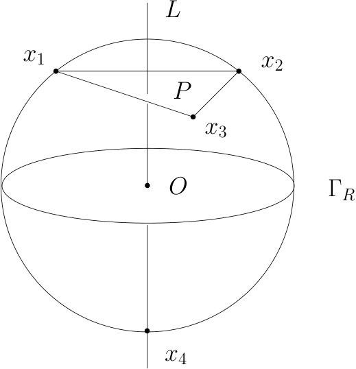 Figure 1
Peer Reviews
No public reviews on file for this paper yet. If you reviewed it on a platform where reviews are public (OpenReview, ICLR, NeurIPS, ICML), you can paste yours below so the community can read it here.
Videos
No videos yet. Explain this paper in a talk, walkthrough, or lecture? Add one.
Inverse moving source problems in
electrodynamics
Guanghui Hu
Beijing Computational Science Research Center, Beijing 100193, China.
,
Yavar Kian
Aix Marseille Univ, Université de Toulon, CNRS, CPT, Marseille, France.
,
Peijun Li
Department of Mathematics, Purdue University, West Lafayette, Indiana 47907, USA.
and
Yue Zhao
School of Mathematics and Statistics, Central China Normal University, Wuhan 430079, China
Abstract.
This paper is concerned with the uniqueness on two inverse moving source problems in electrodynamics with partial boundary data. We show that (1) if the temporal source function is compactly supported, then the spatial source profile function or the orbit function can be uniquely determined by the tangential trace of the electric field measured on part of a sphere; (2) if the temporal function is given by a Dirac distribution, then the impulsive time point and the source location can be uniquely determined at four receivers on a sphere.
1. Introduction
Consider the time-dependent Maxwell equation for the electric field in a homogeneous medium
[TABLE]
which is supplemented by the homogeneous initial conditions
[TABLE]
We assume that the electrodynamic field is excited by a moving point source radiating over a finite time period. Specifically, the source function is assumed to be given in the following form
[TABLE]
where is the source profile function, the temporal function, and is the orbit function of the moving source. Hence the source term is assumed to be a product of the spatially moving source function and the temporal function . Physically, the spatially moving source function can be thought as an approximation of a pulsed signal which is transmitted by a moving antenna, whereas the temporal function is usually used to model the evolution of source magnitude in time. Throughout, we make the following assumptions:
- (1)
The profile function is compactly supported in for some ; 2. (2)
The source radiates only over a finite time period for some , i.e., for and ; 3. (3)
The source moves in a bounded domain, i.e., for all and some .
These assumptions imply that the source term is supported in for . Unless otherwise stated, we always take and set . Denote by the unit normal vector on and let be an open subset with a positive Lebesgue measure.
We study the inverse moving source problems of determining the profile function and the orbit function from boundary measurements of the tangential trace of the electric field over a finite time interval, . Specifically, we consider the following two inverse problems:
- (i)
IP1. Assume that is known, the inverse problem is to determine from the measurement . 2. (ii)
IP2. Assume that is a known vector function, the inverse problem is to determine from the measurement .
The IP1 is a linear inverse problem, whereas the IP2 is a nonlinear inverse problem. The time-dependent inverse source problems have attracted considerable attention [2, 13, 18, 22, 14, 10, 17]. However, the inverse moving source problems are rarely studied for the wave propagation. We refer to [7] on the inverse moving source problems by using the time-reversal method and to [19, 20] for the inverse problems of moving obstacles. numerical methods can be found in [15, 21] to identify the orbit of a moving acoustic point source. To the best of our knowledge, the uniqueness result is not available for the inverse moving source problem, which is the focuse of this paper.
Recently, a Fourier method was proposed for solving inverse source problems for the time-dependent Lamé system [3] and the Maxwell system [8], where the source term is assumed to be the product of a spatial function and a temporal function. These work were motivated by the studies on the uniqueness and increasing stability in recovering compactly supported source terms with multiple frequency data [4, 6, 5, 12, 11, 23, 23]. It is known that there is no uniqueness for the inverse source problems with a single frequency data due to the existence of non-radiating sources [1]. In [3, 8], the idea was to use the Fourier transform and combine with Huygens’ principle to reduce the time-dependent inverse problem into an inverse problem in the Fourier domain with multi-frequency data. The idea was further extended in [9] to handle the time-dependent source problems in elastodynamics where the uniqueness and stability were studied.
In this paper, we use partial boundary measurements of dynamical Dirichlet data over a finite time interval to recover either the source profile function or the orbit function. In Sections 3 and 4.2, we show that the ideas of [3, 8] and [9] can be used to recover the source profile function as well as the moving trajectory which lies on a flat surface. For general moving orbit functions, we apply the moment theory to deduce the uniqueness under a priori assumptions on the path of the moving source, see Section 4.1. When the compactly supported temporal function shrinks to a Dirac distribution, we show in Section 5 that the data measured at four discrete receivers on a sphere is sufficient to uniquely determine the impulsive time point and to the source location. This work is a nontrivial extension of the Fourier approach from recovering the spatial sources to recovering the orbit functions. The latter is nonlinear and more difficult to handle.
The rest of the paper is organized as follows. In Section 2, we present some preliminary results concerning the regularity and well-posedness of the direct problem. Sections 3 and 4 are devoted to the uniqueness of IP1 and IP2, respectively. In Section 5, we show the uniqueness to recover a Dirac distribution of the source function by using a finite number of receivers.
2. The direct problem
In addition to those assumptions given in the previous section, we give some additional conditions on the source functions:
[TABLE]
It follows from [1] that any source function can be decomposed into a sum of radiating and non-radiating parts. The non-radiating part cannot be determined and gives rise to the non-uniqueness issue. By the divergence-free condition of , we eliminate non-radiating sources in order to ensure the uniqueness of the inverse problem. Since the source term has a compact support in , we may show the following result by Huygens’ principle.
Lemma 2.1**.**
It holds that for all .
The proof of Lemma 2.1 is similar to that of Lemma 2.1 in [8]. It states that the electric field over must vanish after time . This property of the electric field plays an important role in the mathematical justification of the Fourier approach.
Noting , taking the divergence on both sides of (1.1), and using the initial conditions (1.2), we have
[TABLE]
and
[TABLE]
Therefore, for all and . In view of the identify , we obtain from (1.1)–(1.2) that
[TABLE]
We briefly introduce some notation on functional spaces with the time variable. Given the Banach space with norm , the space consists of all continuous functions with the norm
[TABLE]
The Sobolev space where both and are positive integers such that , comprises all functions such that exist in the weak sense and belong to . The norm of is given by
[TABLE]
Denote .
Now we state the regularity of the solution for the initial value problem (2.1). The proof follows similar arguments to the proof of Lemma 2.3 in [8] by taking .
Lemma 2.2**.**
The initial value problem (2.1) admits a unique solution
[TABLE]
which satisfies
[TABLE]
where is a positive constant depending on .
Applying the Sobolev imbedding theorem, it follows from Lemma 2.2 that
[TABLE]
Denote by the 3-by-3 identity matrix and by the Heaviside step function. Recall the Green tensor to the Maxwell system (see e.g., [8])
[TABLE]
which satisfies
[TABLE]
with the homogeneous initial conditions:
[TABLE]
Taking the Fourier transform of with respect to the time variable yields
[TABLE]
which is known as the Green tensor to the reduced time-harmonic Maxwell system with the wavenumber . Here is the fundamental solution of the three-dimensional Helmholtz equation and is given by
[TABLE]
It is clearly to verify that satisfies
[TABLE]
3. Determination of the source profile function
In this section we consider IP1. Below we state the uniqueness result. The idea of the proof is to adopt the Fourier approach of [8] to the case of a moving point source.
Theorem 3.1**.**
Suppose that the orbit function is given and that . Then the source profile function can be uniquely determined by the partial data set .
Proof.
Assume that there are two functions and which satisfy
[TABLE]
and
[TABLE]
It suffices to show in if for all .
Let and
[TABLE]
Then we have
[TABLE]
Denote by the Fourier transform of with respect to the time , i.e.,
[TABLE]
By Lemma 2.1, the improper integral on the right hand side of (3.1) makes sense and it holds that
[TABLE]
Hence
[TABLE]
Taking the Fourier transform of (1.1) with respect to the time , we obtain
[TABLE]
Since and , it is clear to note that is analytic with respect to in a neighbourhood of and satisfies the Silver–Müller radiation condition:
[TABLE]
for any fixed frequency . In fact, the radiation condition of can be straightforwardly derived from the expression of in terms of the Green tensor together with the radiation condition of . The details may be found in [8]. Hence, we have on the whole boundary . It follows from (2.2) that
[TABLE]
Let and be the tangential trace of the electric and the magnetic fields in the frequency domain, respectively. In the Fourier domain, there exists a capacity operator such that the following transparent boundary condition can be imposed on (see e.g., [16]):
[TABLE]
This implies that is uniquely determined by on , provided and are radiating solutions. The transparent boundary condition (3.3) can be equivalently written as
[TABLE]
Next we introduce the functions and by
[TABLE]
where is a unit vector and are two unit polarization vectors satisfying . It is easy to verify that and satisfy the homogeneous time-harmonic Maxwell equations in :
[TABLE]
and
[TABLE]
Let with . We have from (3.5) that and . Multiplying both sides of (3.2) by and using the integration by parts over and (3.6), we have from on and the transparent boundary condition (3.4) that
[TABLE]
Hence from (3) we obtain
[TABLE]
By Fubini’s theorem, it is easy to obtain
[TABLE]
Taking the limit yields
[TABLE]
Hence, there exist a small positive constant such that for all ,
[TABLE]
which together with (3.9) implies that
[TABLE]
Similarly, we may deduce from (3.7) and the integration by parts that
[TABLE]
On the other hand, since is compactly supported in and in , we have
[TABLE]
This implies that Since are orthonormal vectors, they form an orthonormal basis in . It follows from the previous identities that
[TABLE]
for all and . Noting that , , are analytical functions in , we obtain for all , which completes the proof by taking the inverse Fourier transform. ∎
4. Determination of moving orbit function
In this section, we assume that the source profile function is given. To prove the uniqueness for IP2, we consider two cases:
Case (i): The orbit is a curve lying in three dimensions;
Case (ii): , where is a plane in three dimensions.
The second case means that the path of the moving source lies on a bounded flat surface in three dimensions. Cases (i) and (ii) will be discussed separately in the subsequent two subsections.
4.1. Uniqueness to IP2 in case (i)
Before stating the uniqueness result, we need an auxillary lemma.
Lemma 4.1**.**
Let be functions such that
[TABLE]
In addition, suppose that
[TABLE]
for all integers . Then it holds that on .
Proof.
Without loss of generality we assume that . Otherwise, we may consider the functions in place of . To prove Lemma 4.1, we first show and then apply the moment theory to get .
Assume without loss of generality that . Write and . Since and , we have . Therefore, there exists sufficiently small positive numbers and such that
[TABLE]
Using the above relations, we deduce from (4.1) that
[TABLE]
which means that
[TABLE]
for all integers . However, since , there exists a sufficiently large integer such that
[TABLE]
Then we obtain
[TABLE]
which is a contradiction. Therefore, we obtain .
Denote and . Since is monotonically increasing, the relation implies that for all and . Using the change of variables, we get
[TABLE]
Hence, it follows from (4.1) that
[TABLE]
where and are two Lebesgue measures such that
[TABLE]
By the Stone–Weierstrass theorem, it is easy to note from (4.2) that , which means
[TABLE]
Introduce two functions
[TABLE]
Hence, from (4.3) we deduce for . Moreover, since , we have and then for , i.e.,
[TABLE]
From (4.4), it is easy to know that for all . Otherwise, suppose at some point . Since for all , we obtain that
[TABLE]
which is a contradiction. Consequently, we obtain and thus for all . The proof is complete. ∎
Our uniqueness result for the determination of is stated as follows.
Theorem 4.2**.**
Assume that is located at the origin and that each component of satisfies for . Then the function can be uniquely determined by the data set .
Proof.
Assume that there are two orbit functions and such that
[TABLE]
and
[TABLE]
Here we assume that and for and . We need to show in if for .
For each unit vector , we can choose two unit polarization vectors such that . Letting and following similar arguments as those of Theorem 3.1, we obtain
[TABLE]
[TABLE]
and
[TABLE]
which means
[TABLE]
Therefore, since , for each unit vector there exists a sequence such that and for each , either or . Hence from (4.5)–(4.6) we have
[TABLE]
Expanding and into power series with respect to , we write (4.7) as
[TABLE]
where
[TABLE]
In view of the fact that , we get
[TABLE]
Since (4.8) holds for all and , it is easy to conclude that for Choosing , we have
[TABLE]
It follows from and Lemma 4.1 that for . Similarly letting and we have and for , respectively, which proves that for . ∎
Remark 4.3**.**
In Theorem 4.2, it states that we can only recover the function over the finite time period because the moving source radiates in this time period, i.e., . The information of for cannot be retrieved. The monotonicity assumption for can be replaced by the following condition: there exist three linearly independent unit directions such that
[TABLE]
Note that this condition can always be fulfilled if the source moves along a straight line with the speed less than one.
4.2. Uniqueness to IP2 in case (ii)
For simplicity of notation, let for and . Let for all . In this subsection, we assume that
[TABLE]
where depends only on and , . Moreover, we assume that does not vanish identically and
[TABLE]
The temporal function is defined the same as in the previous sections. The above assumptions imply that we still have and in . We consider the inhomogeneous Maxwell system
[TABLE]
Since the equation (4.9) is a special case of (1.1), the results of Lemmas 2.1 and 2.2 also apply to this case.
For our inverse problem, it is assumed that is a given source function, where the admissible set
[TABLE]
The -dependent function is also assumed to be given. We point out that these a priori information of and are physically reasonable, while and can be regarded as approximation of the Dirac functions (for example, Gaussian functions) with respect to and , respectively. Our aim is to recover the unknown orbit function which has a upper bound for some and for all . Let and
Below we prove that the tangential trace of the dynamical magnetic field on can be uniquely determined by that of the electric field. It will be used in the subsequent uniqueness proof with the data measured on the whole surface .
Lemma 4.4**.**
Assume that the electric field satisfies
[TABLE]
If on , then on .
Proof.
Let us assume that on and consider defined by
[TABLE]
In view of (4.4) and the fact that on , we find
[TABLE]
We define the energy associated to on
[TABLE]
Since , we have
[TABLE]
It follows that . Moreover, we get
[TABLE]
Integrating by parts in and applying (4.10), we obtain
[TABLE]
This proves that is a constant function. Since
[TABLE]
we deduce for all . In particular, we have
[TABLE]
This proves that
[TABLE]
which implies that on and completes the proof. ∎
In the following lemma, we present a uniqueness result for recovering from the tangential trace of the electric field measured on . Our arguments are inspired by a recent uniqueness result [9] to inverse source problems in elastodynamics. Compared to the uniqueness result of Theorem 4.2, the slow moving assumption of the source is not required in the following Theorem 4.5.
Theorem 4.5**.**
Assume that and the non-vanishing function are both known. Then the function can be uniquely determined by the data set .
Proof.
Assume that there are two functions and such that
[TABLE]
and
[TABLE]
It suffices to show that in if for . Denote and
[TABLE]
Subtracting (4.11) from (4.12) yields
[TABLE]
Since does not vanish identically, we can always find an interval such that
[TABLE]
Set , which is an open set in . We choose a test function of the form
[TABLE]
where is a unit vector, is a unit vector orthogonal to , and are positive constants such that . It is easy to verify that
[TABLE]
Since on , from Lemma 4.4, we also have on . Consequently, multiplying both sides of the Maxwell system by and using integration by parts over we can obtain from (4.15) that
[TABLE]
Note that in the last step we have used Lemma 4.4. Recalling the definition of and , we obtain from the previous identity that
[TABLE]
In view of (4.14) and the choice of , we get
[TABLE]
For a vector , denote by the Fourier transform of with respect to the variable , i.e.,
[TABLE]
Consequently, it holds that
[TABLE]
for all and
On the other hand, since we have . Hence,
[TABLE]
which means for all and Since both and are orthonormal vectors in , they form an orthonormal basis in . Therefore we have
[TABLE]
for all and Since is analytic in and is an open set in , we have for all , which means and then
[TABLE]
for all and This particulary gives
[TABLE]
Assume that there exists one time point such that . By choosing we deduce from (4.16) that
[TABLE]
which is a contradiction to our assumption that . This finishes the proof of for . ∎
Remark 4.6**.**
The proof of Theorem 4.5 does not depend on the Fourier transform of the electromagnetic field in time, but it requires the data measured on the whole surface . However, the Fourier approach presented in the proof of Theorems 3.1 and 4.2 straightforwardly carries over to the proof of Theorem 4.5 without any additional difficulties. Particulary, the result of Theorem 4.5 remain valid with the partial data .
Remark 4.7**.**
In the case of the scalar wave equation,
[TABLE]
where is a scalar function compactly supported on . Then, following the same arguments as in the proof of Theorem 4.5, one can prove that can be uniquely determined by the data set .
5. Inverse moving source problem for a delta distribution
As seen in the previous sections, when the temporal function is supported on , it is possible to recover the moving orbit function for . In this section we consider the case where the temporal function shrinks to the Dirac distribution with some unknown time point . Our aim is to determine and from the electric data at a finite number of measurement points.
Consider the following initial value problem of the time-dependent Maxwell equation
[TABLE]
Since , the electric field in this case can be expressed as
[TABLE]
Before stating the main theorem of this section, we describe the strategy for the choice of four measurement points (or receivers) on the sphere . The geometry is shown in Figure 1. First, we choose arbitrarily three different points . Denote by the uniquely determined plane passing through , and , and by the line passing through the origin and perpendicular to . Obviously the straight line has two intersection points with . Choose one of the intersection points with the longer distance to plane as the fourth point . If the two intersection points have the same distance to , we can choose either one of them as . By our choice of , they cannot lie on one side of any plane passing through the origin, if the plane determined by does not pass through the origin.
Theorem 5.1**.**
Let the measurement positions , be given as above and let be specified as in the introduction part. We assume additionally that and there exists a small constant such that for all and . Then both and can be uniquely determined by the data set , where .
Proof.
Analogously to Lemma 2.1, one can prove that for all and . Taking the Fourier transform of in (3.1) with respect to and making use of the representation of in (5), we obtain
[TABLE]
where . Assume that there are two orbit functions and and two time points and such that
[TABLE]
and
[TABLE]
We need to prove and under the condition for and . Below we denote by one of the measurement points (). Introduce the functions : as follows:
[TABLE]
Since and by our assumption, each component () is either positive or negative in a small neighborhood of , we can obtain that
[TABLE]
Since for some point , from (5) we have
[TABLE]
for all , which means
[TABLE]
Recalling the property of the Fourier transform,
[TABLE]
we deduce from (5.5) that
[TABLE]
Particularly,
[TABLE]
Therefore, we derive from (5) that
[TABLE]
which means
[TABLE]
Physically, the right and left hand sides of the above identity represent the difference of the flight time between and , . Note that the wave speed has been normalized to one for simplicity.
Finally, we prove that the identity (5.6) cannot hold simultaneously for our choice of measurement points (). Obviously, the set represents one sheet of a hyperboloid. This implies that () should be located on one half sphere of radius excluding the corresponding equator, which is a contradiction to our choice of . Then we have and (5.6) then becomes
[TABLE]
This implies that should be on the same plane. This is also a contradiction to our choice of . Then we have . ∎
Remark 5.2**.**
If the source term on the right hand side of (5.1) takes the form
[TABLE]
with the impulsive time points
[TABLE]
One can prove that the set can be uniquely determined by , where . In fact, for , one can prove that can be uniquely determined by , where and .
6. Acknowledgement
The work of G. Hu is supported by the NSFC grant (No. 11671028) and NSAF grant (No. U1530401). The work of Y. Kian is supported by the French National Research Agency ANR (project MultiOnde) grant ANR-17-CE40-0029.
The reference list from the paper itself. Each links out to its DOI / PubMed record.
- 1[1] R. Albanese and P. Monk, The inverse source problem for Maxwell’s equations, Inverse Problems, 22 (2006), 1023–1035.
- 2[2] Yu. E. Anikonov, J. Cheng, and M. Yamamoto, A uniqueness result in an inverse hyperbolic problem with analyticity, European J. Appl. Math., 15 (2004), 533–543.
- 3[3] G. Bao, G. Hu, Y. Kian, and T. Yin, Inverse source problems in elastodynamics, Inverse Problems, 34 (2018), 045009.
- 4[4] G. Bao, P. Li, J. Lin, and F. Triki, Inverse scattering problems with multi-frequencies, Inverse Problems, 31 (2015), 093001.
- 5[5] G. Bao, P. Li, and Y. Zhao, Stability in the inverse source problem for elastic and electromagnetic waves, preprint.
- 6[6] G. Bao, J. Lin, and F. Triki, A multi-frequency inverse source problem, J. Differential Equations, 249 (2010), 3443–3465.
- 7[7] G. Garnier and M. Fink, Super-resolution in time-reversal focusing on a moving source, Wave Motion, 53 (2015), 80–93.
- 8[8] G. Hu, P. Li, X. Liu and Y. Zhao, Inverse source problems in electrodynamics, Inverse Problems and Imaging, 12 (2018), 1411–1428.