Spectrum of random perturbations of Toeplitz matrices with finite symbols
Anirban Basak, Elliot Paquette, Ofer Zeitouni

TL;DR
This paper studies how the eigenvalues of Toeplitz matrices with finite symbols are affected by small random perturbations, showing they converge to a distribution determined by the symbol evaluated on the unit circle.
Contribution
It extends previous results to non-triangular Toeplitz matrices with more general noise, confirming predictions about eigenvalue distributions under perturbations.
Findings
Eigenvalue empirical measure converges to the law of the symbol on the unit circle.
Results apply to non-triangular matrices and non-Gaussian noise.
Confirms pseudo-spectrum predictions for eigenvalue behavior.
Abstract
Let denote an Toeplitz matrix with finite, independent symbol . For a noise matrix satisfying mild assumptions (ensuring, in particular, that at a polynomial rate), we prove that the empirical measure of eigenvalues of converges to the law of , where is uniformly distributed on the unit circle in the complex plane. This extends results from arXiv:1712.00042 to the non-triangular setup and non complex Gaussian noise, and confirms predictions obtained in Reichel and Trefethen (1992) using the notion of pseudo-spectrum.
Click any figure to enlarge with its caption.
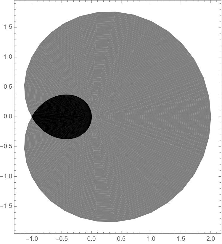 Figure 1
Peer Reviews
No public reviews on file for this paper yet. If you reviewed it on a platform where reviews are public (OpenReview, ICLR, NeurIPS, ICML), you can paste yours below so the community can read it here.
Videos
No videos yet. Explain this paper in a talk, walkthrough, or lecture? Add one.
Spectrum of random perturbations of Toeplitz matrices with finite symbols
Anirban Basak∗
∗International Center for Theoretical Sciences
Tata Institute of Fundamental Research
Bangalore 560089, India
and
Department of Mathematics, Weizmann Institute of Science
POB 26, Rehovot 76100, Israel
,
Elliot Paquette‡
‡Department of Mathematics, The Ohio State University
Tower 100, 231 W 18th Ave, Columbus, Ohio 43210, USA
and
Ofer Zeitouni*§*
*§*Department of Mathematics, Weizmann Institute of Science
POB 26, Rehovot 76100, Israel
and
Courant Institute, New York University
251 Mercer St, New York, NY 10012, USA
(Date: December 14, 2018. Revised November 7, 2019.)
Abstract.
Let denote an Toeplitz matrix with finite, independent symbol . For a noise matrix satisfying mild assumptions (ensuring, in particular, that at a polynomial rate), we prove that the empirical measure of eigenvalues of converges to the law of , where is uniformly distributed on the unit circle in the complex plane. This extends results from [2] to the non-triangular setup and non complex Gaussian noise, and confirms predictions obtained in [16] using the notion of pseudospectrum.
1. Introduction
Let denote the unit circle in the complex plane. Let be a function given by
[TABLE]
where is an absolutely summable complex valued sequence. We denote by the Toeplitz matrix of dimension with symbol , given by
[TABLE]
From the definition it is clear that when is a Laurent polynomial, i.e.
[TABLE]
then is a (finitely) banded Toeplitz matrix which can be thought of as a piece from an infinite Toeplitz matrix; we refer to such matrices as Toeplitz matrices with finite symbols.
For any matrix we denote the empirical measure of its eigenvalues, or equivalently esd, the empirical spectral distribution, by . That is,
[TABLE]
where are the eigenvalues of . In this paper, we find the limit of the empirical spectral distribution (esd) of random perturbations of Toeplitz matrices with finite symbols. This generalizes those results in [2] that deal with triangular Toeplitz matrices with finite symbols (and also with twisted Toeplitz matrices, which we cannot generalize to the non-triangular case, see Remarks 1.7 and 1.9 below). In contrast with [2], we allow for rather general perturbations, as codified in Assumption 1.1.
Assumption 1.1**.**
Let be a sequence of matrices, with possibly complex valued entries, such that the followings hold:
- (i)
[TABLE]
where are the entries of . 2. (ii)
For any , there exists a , depending only on , so that for any fixed deterministic matrix with , we have
[TABLE]
Let denote the law of , where is a random variable uniformly distributed on the unit circle in the complex plane. Equipped with Assumption 1.1 we now state the main result of this paper.
Theorem 1.2**.**
Let be any Toeplitz matrix with a symbol , where is a Laurent polynomial. Assume that satisfy Assumption 1.1. Then, for any , the esd of converges weakly, in probability, to .
Assumption 1.1(i) holds as soon as the second moment of each of the entries (of both complex and real parts) is uniformly bounded. By [15, Theorem 2.1], whenever the entries of are i.i.d. (complex or real) with common -independent distribution having a finite variance, Assumption 1.1(ii) holds. Therefore, Theorem 1.2 holds in that setup. In the next remark, we summarize other cases where Assumption 1.1, and hence Theorem 1.2, hold.
Remark 1.3**.**
Assumption 1.1 holds under various relaxed assumptions on the noise matrix , which we list below.
- (1)
When the entries of are independent and dominated by a single distribution (in the Fourier-analytic sense) that has a -controlled second moment for some , see [15, Definition 2.2 and Remark 2.8]. 2. (2)
When the entries of are independent, satisfy a uniform anti-concentration bound near [math], and have uniform lower bound on the truncated variance, see [4, Lemma A.1]. Furthermore, [15, Theorem 2.9] and [4, Lemma A.1] allow to be a sparse random matrix. 3. (3)
When the entries of have an inhomogeneous variance profile satisfying appropriate assumptions, by a recent result of Cook [6]. Specifically, by [6, Theorem 1.24], the assumption is satisfied when the variance profile is super-regular, see [6, Definition 1.23] for a precise formulation. 4. (4)
When , where is a Haar distributed unitary matrix, see [18, Theorem 1.1].
Remark 1.4**.**
We believe that the sequence in Theorem 1.2 can be replaced by any sequence satisfying . We chose to work with in order to somewhat simplify the proofs.
Remark 1.5**.**
A general notion developed to deal with perturbations of non-normal matrices is that of pseudospectrum, see [17] for an extensive review. This notion provides worse-case estimates and does not focus on the evaluation of limits of empirical measures under random perturbation. However, Theorem 1.2 is consistent with predictions based on pseudospectrum. For a thorough discussion of how pseudospectrum relates to Theorem 1.2, see [2, Section 1.3] and [16].
Our approach to the proof of Theorem 1.2 differs from the one employed in [2], which derived a deterministic equivalence that worked only for complex i.i.d. Gaussian perturbations (in particular, even real Gaussian perturbations are not covered by [2]). Instead, our approach is based on a perturbation idea that can be traced back in this context to [9]. See Section 1.1 below for a further discussion on this.
To describe the approach of this paper we first recall the important notion of logarithmic potential associated with a probability measure .
Definition 1.1** (Log-potential).**
For a probability measure supported on the complex plane define its log-potential as follows:
[TABLE]
As a first step, we will show that there exists a random matrix , with a polynomially decaying spectral norm, such that the conclusion of Theorem 1.2 holds with replaced by .
Theorem 1.6**.**
Let be any Toeplitz matrix with a symbol , where is a Laurent polynomial. Then, there exists a random matrix with
[TABLE]
for some , so that converges weakly, in probability, to . Equivalently, for Lebesgue almost every , , in probability.
Remark 1.7**.**
We do not know the analogue of Theorem 1.6 for the twisted Toeplitz matrices considered in [2], and their non-triangular generalizations. For this reason, we cannot extend Theorem 1.2 to the general banded twisted case. See however Remark 1.9 below for the case of upper triangular twisted Toeplitz matrices.
We next state the replacement principle alluded to above. Here and in the sequel, denotes the open ball in the complex plane of center and radius .
Theorem 1.8** (Replacement principle).**
Let be any deterministic matrix with a bounded operator norm. Suppose and are random matrices. Let be a probability measure on whose support is contained in for some . Assume the following.
- (a)
* and are independent. satisfies (1.1) and satisfies Assumption 1.1. * 2. (b)
For Lebesgue a.e. , the empirical distribution of the singular values of converges weakly, to the law induced by , where . 3. (c)
For Lebesgue a.e. every ,
[TABLE]
Then, for any , for Lebesgue a.e. every ,
[TABLE]
Theorem 1.8 is a generalization of the replacement lemma in [9, Theorem 5], with the advantage that it allows for more general noise models and that it is stated directly in terms of logarithmic potentials and avoids the need to realize the -limit of as a regular element of a non-commutative probability space. It may be of independent interest beyond the study of perturbations of Toeplitz matrices.
Remark 1.9**.**
Theorem 1.8 shows that [2, Theorem 4.1] remains true if one replaces there the complex Gaussian noise by a noise satisfying Assumption 1.1. This can be seen by using in Theorem 1.8 , and using [2, Lemma 4.6] to verify condition (b) of the theorem.
1.1. Related results and extensions
The study of the limiting esd of random perturbations of Toeplitz matrices can be traced back to [7] where in the simplest case of , i.e. when the Toeplitz matrix is the standard Jordan matrix, they derive the limit by studying a relevant Grushin problem. On the other hand [9] derives the limit in the same set-up by first analyzing the limit of the log-potential of the esd of a specific (deterministic) perturbation of the Jordan matrix. Then they use an argument similar in spirit to that of Theorem 1.8 which allows them to replace that specific perturbation by a polynomially vanishing Gaussian perturbation. When the Toeplitz matrix is non-triangular with an arbitrary symbol it is not straightforward to find the required perturbation. Furthermore, it is not clear whether there exists at all some deterministic perturbation allowing one to apply [9, Theorem 5]. Theorem 1.6 of this paper shows that one can indeed find a random perturbation which does that job. Moreover, instead of appealing to [9, Theorem 5] we use Theorem 1.8 which enables us to consider a broad class of random perturbations.
Recently in [2] the limiting spectral distribution of Gaussian perturbation of triangular Toeplitz matrices has been derived by adopting a different strategy. The key to the proof in [2] lies in the following observation: If for Lebesgue a.e. the number of polynomially small singular values of is not too large, where is some sequence of matrices and is the identity matrix, then the limiting esd of Gaussian perturbations of can be described by the Brown measure associated with the limiting operator. So it boils down to finding estimates on the number of small singular values. When , a triangular Toeplitz (or a twisted Toeplitz) matrix, this task has been accomplished in [2]. If is a non-triangular matrix then the approach to finding bounds on the number of small singular values that is used in [2] fail.
Let us add that recent works of Sjöstrand and Vogel [12, 13] also deal with the limiting spectrum of Gaussian perturbations of general Toeplitz matrices. They use yet another strategy which is similar in spirit to the one adopted in [7]. In particular, their methods are robust enough that in [13] they apply them to Toeplitz operators with unbounded symbols.
There are several possible extensions of this paper that one can pursue. For example, one may be interested in understanding finer details of the spectrum, such as the behavior of the outliers of random perturbations of Toeplitz matrices. Building on the ideas of this paper the behavior of the outliers has been studied in a follow-up work [3].
Another interesting question would be to study the limiting esd of random perturbations of Toeplitz matrices with infinite symbols; as mentioned above, for certain perturbations this was achieved in [13]. A careful inspection of the proof of Theorem 1.2 of this paper reveals that one can build on the strategies developed in this paper to consider the case of Toeplitz matrices with a slowly growing bandwidth. For ease of writing and explanation we chose to work with a fixed bandwidth. The case of Toeplitz matrices with a general infinite symbol is at present beyond the scope of our methods.
Outline of the rest of the paper
We will show in Section 3 that Theorem 1.2 is an immediate consequence of Theorems 1.6 and 1.8. In Section 2 we provide the outlines of the proofs of Theorems 1.6 and 1.8. The proofs of these two theorems are carried out in Sections 4 and 5, respectively. Appendix A contains some algebraic results are that are used in the proofs.
Acknowledgements
AB is partially supported by a Start-up Research Grant (SRG/2019/001376) from Science and Engineering Research Board of Govt. of India, and ICTS–Infosys Excellence Grant. OZ is partially supported by Israel Science Foundation grant 147/15 and funding from the European Research Council (ERC) under the European Union’s Horizon 2020 research and innovation program (grant agreement number 692452). We thank the anonymous referees for helpful comments that enhanced the presentation of this paper.
2. Outlines of proofs of Theorems 1.6 and 1.8
We begin with an outline of the proof of Theorem 1.6. From [14, Theorem 2.8.3] and the fact that the support of is compact, it suffices to show that for Lebesgue a.e. in some large compact subset of the complex plane, in probability. Toward this goal, it is useful first to obtain a different representation of the limit.
Lemma 2.1**.**
Let
[TABLE]
for some . For any let be the roots of the polynomial equation
[TABLE]
where . Then, for any ,
[TABLE]
where for , .
The proof of Lemma 2.1 is a straightforward modification of that of [2, Lemma 4.3]. We omit the details.
We next sketch the proof of Theorem 1.6, in the special case where is the Toeplitz matrix with symbol . Set where . By Lemma 2.1, the form of limiting log potential depends on the number of roots of the polynomial greater than one in modulus. This yields (open) regions , , whose boundaries have zero Lebesgue measure and the closure of whose union is , so that for all there are exactly roots of the equation that are greater than one in modulus. Thus, to establish Theorem 1.6 we need to find a noise matrix such that the following holds:
[TABLE]
where and are the roots of the relevant equation arranged in the non-increasing order of their moduli. We refer the reader to Figure 1 for an illustration of the regions .
(We will see later that it is enough to consider the noise supported on the lower left elements .)
To derive (2.2), we expand the determinant of . The latter can be written as a linear combination of products of determinants of various sub-matrices of and (see Lemma A.1 below). We identify the dominant term in this expansion, as follows. Let denote the sub-matrix of induced by the rows and the columns indexed by and , respectively. Recalling Widom’s theorem concerning the determinant of a finitely banded Toeplitz matrix (see [11, 19]), we obtain
[TABLE]
where we write to indicate that there exists some absolute constant such that , for all large .
From (2.3) we see that if or then there are sub-matrices of whose determinants are of larger magnitude than that of . We also note that the expansion of has terms that are products of determinants of these sub-matrices and the determinant of relevant sub-matrices of the noise matrix (of fixed dimension), where the latter can be chosen to be non-zero and only polynomially (in ) decaying. It follows that if the determinants of those sub-matrices of are of maximal exponential growth among the determinants of all possible sub-matrices of , then converges to the limit in (2.2). This not only explains how the limit arises but also identifies potential candidates for the dominant terms (depending on the location of in the complex plane) in the expansion of the determinant, and gives a heuristic for the proof of Theorem 1.6.
To justify this heuristic and obtain an actual proof of Theorem 1.6 in the case under consideration, it is natural to extend (2.3) and claim that
[TABLE]
for some large absolute constant , with large probability, where is the homogeneous polynomial of degree in the entries of , in the expansion of the determinant of . In (2.4) we have used the standard notations and to denote and , respectively. Finding bounds on requires the same for for all subsets such that . As is not necessarily a Toeplitz matrix for arbitrary choices of we can no longer rely on Widom’s result. We overcome this obstacle by noting that any upper triangular finitely banded Toeplitz matrix can be represented as a product of bidiagonal matrices, where the bidiagonal matrices depend on the roots of polynomial equation associated with the symbol of the Toeplitz matrix in context. Since the determinant of any sub-matrix of a bidiagonal matrix is easily computable (see Lemma A.3) one can then use the Cauchy-Binet theorem to find a bound on . Using this and some combinatorial arguments, we then obtain the desired bound on whenever the entries of are uniformly polynomially vanishing.
We emphasize that the approach described above generalizes easily to triangular finitely banded Toeplitz matrix. The general case requires a modification, since non-triangular Toeplitz matrices cannot be decomposed into a product. We resolve this issue by using the following simple key observation: any Toeplitz matrix with finite symbol can be viewed as a sub-matrix of an upper triangular Toeplitz matrix with an another finite symbol of a slightly larger dimension. Using this observation, we can then follow the same scheme as described above to find an upper bound on .
To complete the proof of (2.4) we then need to find a lower bound on the predicted dominant term, . This is obtained using an anti-concentration estimate, which is shown to hold whenever the entries of are assumed to have a bounded density, which we will impose since the matrix is an auxilliary matrix and does not appear in the statement of our main theorem, Theorem 1.2. See Lemma 4.1 and Proposition 4.5. This will prove (2.4). To finish the proof of Theorem 1.6, we then obtain an (easy) matching upper bound on .
We next outline the proof of Theorem 1.8. It suffices to show that for Lebesgue a.e. in a compact subset of ,
[TABLE]
Using the assumptions of Theorem 1.8 and standard perturbation results for the spectrum of Hermitian matrices, it readily follows that and , the empirical distributions of the singular values of and , respectively, have the same limit, and that limit is , the law of where . As is unbounded both near [math] and , the limit in (2.5) is not immediate from this. Using bounds on the Hilbert-Schmidt norms of the relevant matrices the singularity near can be taken care of. Treating the singularity of near [math] involves two steps. As the integral of near zero, with respect to is negligible, using assumptions (b)-(c) the same can be shown to hold for . Hence, it suffices to show that the integral of on the interval with respect to goes to zero as .
The latter is obtained by standard arguments, as follows. We use Assumption 1.1(ii) to deduce that it is enough to integrate in for some small constant . Now, using bounds on Hilbert-Schmidt norms of and one can derive a bound on the difference of the Stieltjes transforms of and . Using this, one obtains that the difference of the total mass of any interval near zero, under and , is negligible. Upon using an integration by parts, this gives the required control on the integral of near [math] under and completes the proof.
3. Proof of Theorem 1.2 using Theorems 1.6 and 1.8
We will take provided by Theorem 1.6, set in Theorem 1.8, and verify that the hypotheses of the latter hold. Clearly, has uniformly bounded operator norm. The assumption (a) is obvious. To see that assumption (b) holds, it is enough to check that for positive integer,
[TABLE]
To check (3.1) we first note that
[TABLE]
where is the nilpotent matrix given by given by . Using this observation we then expand and find out the limit of each term in term in that expansion. To work out this step we need to introduce some notation.
Let and with non-negative integers bounded by , and set . We say that is balanced if . Using (3.2) we find that
[TABLE]
for appropriate coefficients , while
[TABLE]
with the same coefficients . Note that
[TABLE]
if is not balanced, while
[TABLE]
if is balanced. Similarly, equals if is balanced, and vanishes otherwise. Combining these facts, we obtain (3.1), and thus verify that assumption (b) holds.
Assumption (c) holds because, from Theorem 1.6, we see that for Lebesgue a.e. ,
[TABLE]
We have checked all assumptions of Theorem 1.8; applying the latter we conclude that for Lebesgue a.e. and for any ,
[TABLE]
By the proof of [14, Theorem 2.8.3] and the fact that the support of is compact, this implies the convergence in probability of to in the vague topology, and hence in the weak topology. ∎
4. Proof of Theorem 1.6
In this section we prove Theorem 1.6. As outlined in Section 2, the key is to establish (2.4). Turning to this task, introduce, for any ,
[TABLE]
where , , and for is the permutation on which places all the elements of before all the elements of , but preserves the order of the elements within the two sets. Define
[TABLE]
To prove Theorem 1.6 we will choose which satisfies the following band structure:
[TABLE]
where denotes the -th entry of . That is, has non-zero entries only in its lower left and upper right corners, and the widths of those corners are determined by and , respectively. As indicated in (2.3) such a band structure is necessary (as we will see it is also sufficient) to have a non-zero contribution from the sub-matrices of whose determinants are of larger magnitudes compared to that of the whole matrix, in the expansion of . Recall from (2.2)-(2.3) that the dominant term depends on the number of roots of of (2.1), that are greater than one in modulus. Hence, we split the complex plane into regions according to the number of roots of with modulus greater than one, using the following notation.
Let , 111Hereafter will denote the roots of the equation . This change in notation is adopted to avoid the unnecessary appearance of signs in the determinant of the sub-matrices of ., be the roots of the equation , arranged so that . For , let denote the number of roots of the equation that are greater than or equal to one in moduli. Fixing , for we define
[TABLE]
Note that
[TABLE]
If for some then we also have that
[TABLE]
Therefore is contained in a set of Lebesgue measure zero and hence it is enough to consider . Further let be the set of ’s for which admits a double root. It follows from [5, Lemma 11.4] that the cardinality of is at most finite.
The next lemma identifies the dominant term in the expansion of .
Lemma 4.1**.**
Fix such that . Let be such that
[TABLE]
for some , where are uniformly bounded real valued independent random variables with uniformly bounded densities with respect to the Lebesgue measure. Then, for Lebesgue a.e. , and any ,
[TABLE]
where an empty product by convention is set to one.
Lemma 4.1 yields a lower bound on the order of the magnitude of the predicted dominant term in the expansion of . Next we need to show that the sum of the rest of the terms is of smaller order. To show this, we split it into two sums: and . The second sum will be shown to be polynomially small compared to the leading term, whereas the first will be shown to be exponentially small. This is the content of the two following lemmas.
Lemma 4.2**.**
Let , and be as in Lemma 4.1. Then, for Lebesgue a.e. ,
[TABLE]
Lemma 4.3**.**
Under the same set-up as in Lemma 4.2, for Lebesgue a.e. , we have
[TABLE]
for some small constant .
The proofs of Lemmas 4.2 and 4.3 are in Section 4.1, while the proof of Lemma 4.1 is postponed to Section 4.2. To complete the proof of Theorem 1.6, we will also need an upper bound on the dominant term, which is contained in the next lemma, whose proof is deferred to Section 4.2.
Lemma 4.4**.**
Under the same set-up as in Lemma 4.1, for Lebesgue a.e. , there exists a constant depending on and only, so that
[TABLE]
Equipped with these four lemmas, we now compete the proof of Theorem 1.6.
Proof of Theorem 1.6.
From the definition of it follows that there are at most non-zero entries in each row of . Furthermore, each entry of is at most . Therefore, by the Gershgorin circle theorem, it follows that , establishing the desired property (1.1). Next, as in the proof of Theorem 1.2, the weak convergence of to follows from the convergence, for Lebesgue a.e. , of the log-potentials:
[TABLE]
To this end, recalling the definition of from (4.1) and applying Lemma A.1 we have that
[TABLE]
for any integer between and . Setting in Lemma 4.1 and combining Lemmas 4.1-4.3 we note that for Lebesgue a.e. , there exists an event of probability at least such that, on that event, we have
[TABLE]
for all large . This in turn implies that
[TABLE]
for Lebesgue a.e. every . Finally combining Lemmas 4.1 and 4.4 we obtain that for Lebesgue a.e. every ,
[TABLE]
Combining (4.5)-(4.7) we now deduce (4.4) for Lebesgue a.e. and any integer such that . This completes the proof. ∎
4.1. Upper bound on non-dominant terms
Recall from Section 2 that to establish bounds on the predicted non-dominant terms, one uses the fact any upper triangular Toeplitz matrix with a finite symbol can be expressed as a product of bidiagonal matrices. To use the same representation for a non-triangular Toeplitz matrix we view it as a sub-matrix of an upper triangular Toeplitz matrix of a slightly larger dimension. Toward this end, we introduce the folowing definition.
Definition 4.1** (Toeplitz with a shifted symbol).**
Let be a Toeplitz matrix with finite symbol and as before . For such that and , set to be the Toeplitz matrix with first row and column
[TABLE]
respectively, where , . That is,
[TABLE]
From Definition 4.1, it follows that
[TABLE]
Note that is an upper triangular Toeplitz matrix. Since are the roots of the equation we obtain that
[TABLE]
where we recall that is the nilpotent matrix given by , for .
Hence, recalling the definition of from (4.1), applying the Cauchy-Binet theorem, and writing for any set of integers and an integer , we obtain that
[TABLE]
where
[TABLE]
and for any set . Equipped with this preparatory decomposition of , we are now ready to step into the proof of Lemma 4.2.
Proof of Lemma 4.2.
From the definition of the noise matrix it follows that the number of non-zero rows (and also non-zero columns) in is at most . This means that for any . Therefore, it is enough to show that (4.3) holds with the sum in the numerator being replaced by , where .
To achieve this, we need to simplify (4.8); this simplification, summarized in (4.12) and (4.13) below, will also be useful in the proof of Lemma 4.3. From (4.8)-(4.9), we see that each is of cardinality . Therefore, we write
[TABLE]
and for brevity we also denote . Applying Lemma A.3 we see that
[TABLE]
only when for some with , , where
[TABLE]
Since
[TABLE]
we have the following following equivalent representation of :
[TABLE]
where
[TABLE]
We also note that in (4.8) the outer sum is over and due to the constraint (4.9) we only need to consider , where
[TABLE]
Thus applying Lemma A.3 again, from (4.8) we now deduce that
[TABLE]
where
[TABLE]
[TABLE]
Returning to the proof of the lemma, it suffices to bound . Turning to this task, we assume without loss of generality that . This implies that
[TABLE]
for every such that . On the other hand, the definition of and the fact that imply that there are no roots of on the unit circle, hence we deduce that there exists , such that
[TABLE]
Hence,
[TABLE]
where the last inequality follows from the fact that . To finish the proof it remains to find an upper bound on the cardinality of . We claim that
[TABLE]
Equipped with (4.17), it now follows from (4.16) that
[TABLE]
Since implies that are bounded away from zero, (4.18) together with (4.12) yield (4.3).
It remains to establish the bound (4.17). To this end, set
[TABLE]
For the to satisfy , we observe that the ’s can be chosen in at most
[TABLE]
ways. Next, recall that implies that
[TABLE]
Thus, and automatically fix . Since the number of choices of is at most , as , for all large , the claim (4.17) follows from (4.20). The proof of the lemma is now complete. ∎
Next we show that for the sum is of smaller order compared to the dominant term .
Proof of Lemma 4.3.
We first claim that for any , the set (see (4.11)) being nonempty forces either or to be close to , depending on whether or . This observation will be then combined with the bounds (4.15) and (4.17) to complete the proof.
Consider first the case . For any we have that and hence for any ,
[TABLE]
As for and , it further implies that if then we must have
[TABLE]
Next we consider the case . For any we have that . Therefore
[TABLE]
On other hand, we have that for . Since for any , and are integers, using induction, we further obtain that
[TABLE]
for any . As we find that . Hence, from (4.23) we deduce that
[TABLE]
for any . Noting that for all , we obtain
[TABLE]
Thus, (4.22) and (4.24) implies that, if then
[TABLE]
To complete the proof of the lemma we now use (4.13)-(4.15) and (4.17) to conclude that for any ,
[TABLE]
for all large , for some sufficiently small , depending only on and . The proof finishes upon using (4.12). ∎
4.2. Lower and upper bounds on the dominant term
We will first prove Lemma 4.1, which is a lower bound on the dominant term. The proof is based on the following elementary anti-concentration bound for homogeneous polynomials of independent random variables, which may be of independent interest.
Proposition 4.5**.**
Fix and let be a sequence of independent real-valued random variables, whose law possesses a density with respect to the Lebesgue measure which is uniformly bounded by one. Let be a homogenous polynomial of degree such that the degree of each variable is at most one. That is,
[TABLE]
for some collection of complex valued coefficients , where denotes the set of all distinct elements of .
Assume that there exists an such that for some absolute constant . Then for any we have
[TABLE]
Proof.
As the densities of are uniformly bounded by one, the desired anti-concentration property is immediate for . To prove the general case, we proceed by induction. To this end, we introduce some notation. Order the elements of and denote them by . For , define . Set
[TABLE]
For , we iteratively define
[TABLE]
Equipped with the above notations we see that
[TABLE]
and . We will prove inductively that
[TABLE]
from which the desired anti-concentration bound follows by taking . Hence, it only remains to prove (4.25).
For , is a homogeneous polynomial of degree in the variables , and (4.25) follows from the assumptions on and the fact that . Assuming that (4.25) holds for and fixing , we have that with ,
[TABLE]
where we have used the fact that and are independent of , and the bound on the density for the latter. Using integration by parts, for any probability measure supported on we have that
[TABLE]
Therefore, using the induction hypothesis,
[TABLE]
Since for we have that , combining the above with (4.2) and setting we establish (4.25) for . This completes the proof. ∎
Equipped with Proposition 4.5 we now begin the proof of Lemma 4.1.
Proof of Lemma 4.1.
Recalling (4.1) we note that is a homogeneous polynomial of degree in the entries of the noise matrix such that the degree of each entry of is one. Therefore, to apply Proposition 4.5 we only need to show that there exists with such is bounded below. The choice of such subsets will depend on the sign of . Hence, the proof is split into two cases.
Considering the case we set and . Recalling Definition 4.1 we find that
[TABLE]
We apply Widom’s result on the determinant of finitely banded Toeplitz matrices, in particular [5, Theorem 2.8] to deduce that for any , one has
[TABLE]
for some collection of coefficients , where recall that is the collections of ’s such that has double roots. Furthermore, the coefficients are bounded both below and above, for any . As and , using (4.15) we therefore deduce that there exists some small positive constant so that, for all large ,
[TABLE]
From the definition of it follows that for the above choices of and the determinant of , ignoring the factor , is a homogeneous polynomial of degree of independent uniformly bounded random variables with uniformly bounded densities. Therefore, we are in a position to apply Proposition 4.5.
Without loss of generality, assuming that the densities of are uniformly bounded by one, we apply Proposition 4.5 for
[TABLE]
with and to arrive at (4.2) for any . As contains at most finitely many points this proves the lemma when .
Turning to prove the same for , we reverse the roles of and . That is, we now set and and follow the same steps as above.
For the proof is straightforward. From its definition we have . Upon setting in (4.27) the result is immediate. Now the proof of the lemma is complete. ∎
We end this section with the proof of Lemma 4.4. Its proof is very similar to that of Lemma 4.2. Hence, only an outline is provided.
Proof of Lemma 4.4.
We split the proof into two cases: and . First, let us consider . As we find from (4.12)-(4.15) and (4.17) that
[TABLE]
If then the desired result follows from Widom’s result (see [5, Theorem 2.8]). ∎
5. Proof of Theorem 1.8
We recall from Section 2 that to prove Theorem 1.8 it suffices to establish (2.5). As outlined there, the key to the latter is to bound the difference of the mass of intervals near zero under the measures and , the empirical distribution of the singular values of and , respectively, where . This in turns will be achieved by controlling the differences of the Stieltjes transforms of the corresponding measures. So, we begin this section with its definition.
Definition 5.1**.**
The Stieltjes transform of a probability measure on is defined as
[TABLE]
To obtain a bound on the probability of any interval under from that of we use the following two inequalities. These are a consequence of [9, Eqns. (6)-(8)]: for any , and such that we have
[TABLE]
and
[TABLE]
Now to find a difference of the Stieltjes transforms of and we also need the symmetrized form of the Stieltjes transform, as follows. For a matrix , define
[TABLE]
and the Stieltjes transform
[TABLE]
is the Stieltjes transform of the symmetrized version of the empirical measure of the singular values of . Equipped with the above notation we have the following lemma.
Lemma 5.1**.**
For and any matrices,
[TABLE]
where denotes the Hilbert-Schmidt norm.
Proof.
Using the resolvent identity we have that
[TABLE]
Recall the following version of the Cauchy-Schwarz inequality: for any two matrices and
[TABLE]
Since for any Hermitian matrix one has , the claim follows from (5.5) upon using (5.6) with and . ∎
As a last preliminary step, we need the following easy lemma.
Lemma 5.2**.**
For any probability measure ,
[TABLE]
for Lebesgue almost every .
Proof.
For , set . Fix . Note that, by Fubini’s theorem,
[TABLE]
In particular, for any , with , we obtain that
[TABLE]
In particular, . Using the monotonicity of , we conclude that for Lebesgue almost every , . Taking a sequence gives (5.7), first for Lebesgue almost every , and then for almost every . ∎
We are now ready to prove Theorem 1.8.
Proof of Theorem 1.8.
To establish (1.3) we first claim that , in probability, for Lebesgue a.e. , where is the law of and . The argument is similar to that employed in the proof of Theorem 1.2. Write and . We have that by assumption (b), while Assumption 1.1(i) and Markov’s inequality imply that
[TABLE]
for any . On the other hand, by the Hoffman-Wielandt inequality, see [1, Lemma 2.1.19], the map , viewed as a map from the space of Hermitian matrices equipped with the normalized Hilbert-Schmidt norm to the space of probability measures equipped with the weak topology, is continuous. Note that for any matrix, the singular values of are the same as the modulus of the eigenvalues of the matrix
[TABLE]
up to double the multiplicity for each singular value. In particular,
[TABLE]
in probability, by (5.8). We conclude from that and the above mentioned continuity of the empirical measure in the (normalized) Hilbert-Schmidt norm that
[TABLE]
as claimed.
To complete the proof we need to extend the convergence of to the convergence of the integral of against this measure. To this end, using (5.8) again and the fact that the operator norm of is bounded, we see that there exists a compact set such that for any
[TABLE]
Hence, for any ,
[TABLE]
for Lebesgue a.e. . Note that
[TABLE]
Thus, (5.7) together with (5.9) imply that it only remains to show that given any , there exists such that for any
[TABLE]
for Lebesgue a.e. and some large constant . To prove this, we first show that an analogue of (5.10) holds for the empirical measure of the singular values of .
Turning to do this task, using (1.1) and arguing similarly to the steps leading to (5.9), we obtain that
[TABLE]
for Lebesgue a.e. , and further, for any ,
[TABLE]
for Lebesgue a.e. . Together with assumptions (b)-(c), we conclude that for Lebesgue a.e. , given any , there exists such that for all ,
[TABLE]
Having shown (5.12) we now proceed to the proof of (5.10). Using Assumption 1.1(ii) we see that there exists a sufficiently large constant such that
[TABLE]
where is the minimal singular value of a matrix . Hence,
[TABLE]
Now to control the integral of over we apply (5.4) to deduce that
[TABLE]
on the event
[TABLE]
where and .
Let and denote the symmetrized versions of the probability measures and , respectively. Setting , , and using (5.1)-(5.2) and (5.14) in the second inequality, we have that
[TABLE]
on , for all large , where in the third inequality we used the symmetry of and .
It remains to bound the integral of over . Toward this, using integration by parts we note that, for and any probability measure on ,
[TABLE]
Arguing as in (5.15) we obtain
[TABLE]
where in the last step we have used the fact that for any , and a change of variables. Similar reasoning yields that
[TABLE]
Thus combining (5.15), and (5.17)-(5.18), and using (5.16) we deduce that for sufficiently small and all large ,
[TABLE]
on the event , where is some large constant. Finally, (5.8) and (1.1) imply that . Therefore, combining (5.12) and (5.13), the claim in (5.10) now follows. This completes the proof of the theorem. ∎
Appendix A Some algebraic facts
In this section we collect a couple of standard matrix results which have been used in the proofs appearing in Section 4.
The first result shows that the determinant of the sum of the two matrices can be expressed as a linear combination of products of the determinants of appropriate sub-matrices. The proof follows from the definition of the determinant, see e.g. [10]. We adopt the convention that the determinant of the matrix of size zero is one. For an matrix , and we write for the sub-matrix of which consists of the rows in and the columns in .
Lemma A.1**.**
For any matrices and we have
[TABLE]
where , and for is the permutation on which places all the elements of before all the elements of , but preserves the order of elements within the two sets.
The next lemma evaluates the determinant of any sub-matrix of a bidiagonal matrix.
Lemma A.2** ([8, Lemma 2.2]).**
Let be an upper bi-diagonal matrix and such that . Then equals the product of the diagonal entries of .
The next lemma, which follows readily from Lemma A.2, evaluates the determinant of any sub-matrix of a bidiagonal Toeplitz matrix.
Lemma A.3** ([8, Lemma 2.3]).**
Let , , , and . Then, with ,
[TABLE]
The reference list from the paper itself. Each links out to its DOI / PubMed record.
- 1[1] Greg W. Anderson, Alice Guionnet, and Ofer Zeitouni. An introduction to random matrices . No. 118. Cambridge University Press, 2010.
- 2[2] A. Basak, E. Paquette, and O. Zeitouni. Regularization of non-normal matrices by Gaussian noise - the banded Toeplitz and twisted Toeplitz cases. Forum of Mathematics, Sigma , 7 , E 3, 2019.
- 3[3] A. Basak and O. Zeitouni. Outliers of random perturbations of Toeplitz matrices with finite symbols. Ar Xiv preprint , ar Xiv:1905.10244, 2019.
- 4[4] C. Bordenave and D. Chafaï. Around the circular law. Probability Surveys , 9 , 1–89, 2012.
- 5[5] A. Böttcher and S. M. Grudsky. Spectral Properties of Banded Toeplitz Matrices . Vol. 96, Siam, 2005.
- 6[6] N. Cook. Lower bounds for the smallest singular value of structured random matrices. The Annals of probability , 46 (6), 3442–3500, 2018.
- 7[7] R. B. Davies and M. Hager. Perturbations of Jordan matrices. Journal of Approx.imation Theory 156 , 82–94, 2009.
- 8[8] O. N. Feldheim, E. Paquette, and O. Zeitouni. Regularization of non-normal matrices by Gaussian noise. International Mathematics Research Notices 18 , 8724–8751, 2015.