Extraction of the CKM phase $\gamma$ using charmless 3-body decays of $B$ mesons
Emilie Bertholet, Eli Ben-Haim, Bhubanjyoti Bhattacharya, Matthew, Charles, David London

TL;DR
This paper extracts the CKM phase gamma from charmless three-body B meson decays using amplitude analyses and flavor symmetry assumptions, finding multiple solutions with one consistent with the Standard Model.
Contribution
It applies a novel method to determine gamma from three-body B decays, incorporating amplitude analyses and SU(3) symmetry, revealing multiple solutions including the Standard Model compatible one.
Findings
Six solutions found for gamma, with one compatible with the Standard Model.
SU(3) symmetry breaking effects are at the percent level.
The method demonstrates feasibility of extracting gamma from complex decay modes.
Abstract
The weak phase is extracted from three-body charmless decays of mesons following a method proposed by Bhattacharya, Imbeault \& London. The result is obtained by combining the BABAR amplitude analyses for the processes , , , and , under the assumption of flavour symmetry. Six possible solutions are found. One solution is compatible with the Standard Model while the others are not. It is also found that, when averaged over the entire Dalitz plane, the effect of breaking on the analysis is only at the percent level.
Click any figure to enlarge with its caption.
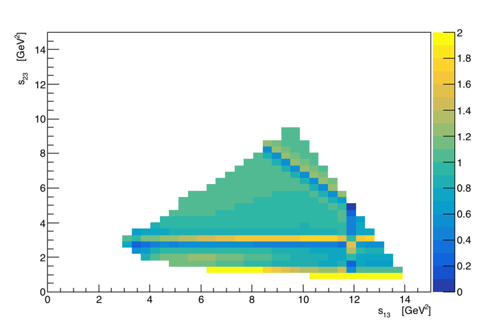 Figure 1
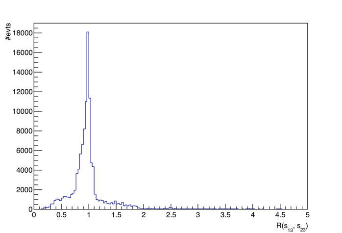 Figure 2
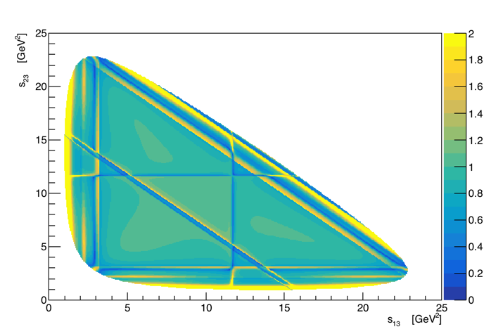 Figure 3
 Figure 4
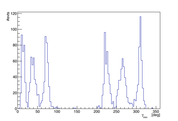 Figure 5
| Minimum 1 | |||
|---|---|---|---|
| Minimum 2 | |||
| Minimum 3 | |||
| Minimum 4 | |||
| Minimum 5 | |||
| Minimum 6 |
| Count | Fraction (%) | |
|---|---|---|
| Minimum 1 | 484 | 96.6 |
| Minimum 2 | 474 | 94.6 |
| Minimum 3 | 461 | 92.0 |
| Minimum 4 | 499 | 99.6 |
| Minimum 5 | 487 | 97.2 |
| Minimum 6 | 488 | 97.4 |
| Poorly resolved minima | Flavour breaking | |
|---|---|---|
| Minimum 1 | ||
| Minimum 2 | ||
| Minimum 3 | ||
| Minimum 4 | ||
| Minimum 5 | ||
| Minimum 6 |
| 12° | 1.06 |
| 37° | 1.06 |
| 68° | 1.05 |
| 223° | 1.06 |
| 266° | 1.05 |
| 307° | 1.05 |
| Count | Fraction (%) | |
|---|---|---|
| minimum 1 | 306 | 76.3 |
| minimum 2 | 329 | 82.0 |
| minimum 3 | 372 | 92.3 |
| minimum 4 | 383 | 95.5 |
| minimum 5 | 378 | 94.3 |
| minimum 6 | 391 | 97.5 |
| Minimum 1 | |||||
| Minimum 2 | |||||
| Minimum 3 | |||||
| Minimum 4 | |||||
| Minimum 5 | |||||
| Minimum 6 |
Peer Reviews
No public reviews on file for this paper yet. If you reviewed it on a platform where reviews are public (OpenReview, ICLR, NeurIPS, ICML), you can paste yours below so the community can read it here.
Videos
No videos yet. Explain this paper in a talk, walkthrough, or lecture? Add one.
Extraction of the CKM phase using charmless 3-body decays of mesons
Emilie Bertholet
LPNHE, Sorbonne Université, Paris Diderot Sorbonne Paris Cité, CNRS/IN2P3, Paris, France
Eli Ben-Haim
LPNHE, Sorbonne Université, Paris Diderot Sorbonne Paris Cité, CNRS/IN2P3, Paris, France
Bhubanjyoti Bhattacharya
Department of Natural Sciences, Lawrence Technological University, Southfield, MI 48075, USA
Matthew Charles
LPNHE, Sorbonne Université, Paris Diderot Sorbonne Paris Cité, CNRS/IN2P3, Paris, France
David London
Physique des Particules, Université de Montréal,
C.P. 6128, succ. centre-ville, Montréal, QC, Canada H3C 3J7
Abstract
The weak phase is extracted from three-body charmless decays of mesons following a method proposed by Bhattacharya, Imbeault & London. The result is obtained by combining the BaBar amplitude analyses for the processes , , , and , under the assumption of flavour symmetry. Six possible solutions are found:
[TABLE]
One solution is compatible with the Standard Model while the others are not. It is also found that, when averaged over the entire Dalitz plane, the effect of breaking on the analysis is only at the percent level.
1 Introduction
In the Standard Model (SM), violation in the weak sector is due to a complex phase in the Cabibbo-Kobayashi-Maskawa (CKM) matrix. The CKM matrix is and unitary; its phase information is often represented as a triangle in the complex plane, the Unitarity Triangle [1]. Its three interior angles , and sum to , and each contains information about the complex phase. In order to test the SM, one measures , and in many different ways. Any discrepancies would suggest the presence of physics beyond the SM.
To date, direct searches for this New Physics (NP) have not found anything, implying that the mass scale of the NP may be beyond the reach of present experiments. However, these new particles can still contribute significantly to loop processes, so that flavour physics, which is sensitive to such virtual effects, is a very promising avenue to perform indirect searches for NP.
Of the three angles of the Unitarity Triangle, is currently the least well known: the world average value is [2]. It has mainly been extracted using processes dominated by tree-level transitions such as [3, 4, 5]. One potential way of searching for NP would therefore be to measure via loop-level processes. This can be done using charmless three-body decays ( is a pseudoscalar meson) [6, 7].
The method proposed in Ref. [8] uses flavour symmetry to relate and decays. The angle is then obtained by combining information from the Dalitz plots for , , , , and . These decay modes all involve transitions and include contributions from both tree and penguin (loop) diagrams (the inclusion of charge-conjugate decay modes is implied throughout this paper). The extraction of is therefore potentially sensitive to NP.
A preliminary implementation of this method was carried out in Ref. [9] using published BaBar results. In the present paper, we repeat the analysis of the same results, while fully taking into account the experimental uncertainties and their correlations. We find six possible solutions for . One agrees with the world-average (Standard Model) value for gamma; the other solutions do not, so that a NP scenario is allowed by the data. We are also able to estimate the size of breaking. We find that local -breaking effects can reach the usual level, especially near resonances. However, when averaged over the entire Dalitz plane, the net effect of breaking is only at the percent level.
We begin in Sec. 2 with a review of the method for extracting from and decays. Practical details of how to implement this method are discussed in Sec. 3. In Sec. 4 we present the results of the analysis where is extracted from four decay modes, assuming no breaking. Systematic uncertainties are discussed in Sec. 5. Sec. 6 contains a description of further tests of breaking. We conclude in Sec. 7.
2 Method of extraction of
We begin with a review of the method for extracting from and decays. There are several ingredients. First, the amplitudes for three-body decays can be written in terms of diagrams [6, 10]. These diagrams are similar to those of two-body decays [11, 12], except that here it is necessary to “pop” a quark pair from the vacuum. Also, in contrast to two-body diagrams, the three-body diagrams are momentum dependent.
Second, one can fix the symmetry of the final state in by using its Dalitz plot [6]. We define the three Mandelstam variables , where is the momentum of , and 123 231 or 312. (These obey .) Experimentally, one can reconstruct the decay amplitude , which varies as a function of position in the Dalitz plot. The amplitude that is fully symmetric under permutations of the final-state particles is then given by
[TABLE]
The symmetrised amplitude has a sixfold symmetry in the Dalitz plane. In effect, the plane can be divided into six regions; the structure and information in each region is identical to the others. It is therefore sufficient to consider points in one sixth of the symmetrised Dalitz plane.
Third, in Ref. [7] it was shown that, as is the case in two-body decays [13, 14, 15], under flavour there are relations between the electroweak penguin (EWP) and tree diagrams for transitions. For the fully-symmetric final state, these take the form
[TABLE]
where the are Wilson coefficients and (the are elements of the CKM matrix).
The method uses and decays. In the diagrams, the quark pair popped from the vacuum is or (under isospin, these diagrams are equal). On the other hand, the diagrams have a popped pair. Now, under flavour symmetry, which is required for the EWP-tree relations eq. (2), diagrams with a popped quark pair are equal to those with a popped or . In other words, under the diagrams in decays are the same as those in decays.
Of course, flavour symmetry is not exact, so one must keep track of breaking. Technically, there will be an -breaking factor for each diagram. However, if all such quantities are included, there will be too many unknown parameters to perform a fit. For this reason, we make the assumption that the size of breaking is the same for all diagrams, so there is a single -breaking parameter relating and decays ( corresponds to the flavour- limit). The idea behind this assumption is as follows. As noted above, the diagrams are momentum dependent. This means that the size of breaking associated with a particular diagram, , varies from point to point on the Dalitz plot. Specifically, will be at some points and at others. When one averages over all points, will be small, and this will be true for all diagrams. For this reason, we make the assumption that the size of breaking is the same for all diagrams, and we expect it to be small. As we will see, in our fits is found to be at the percent level, which supports our assumption.
Three and two decays are used in this analysis. They are , , , , and . (Note that both and are observed as .) As shown in Ref. [9], when the EWP-tree relations of eq. (2) are used, the fully-symmetric amplitudes for the five modes can be expressed as linear combinations of five effective diagrams:
[TABLE]
Here the complex parameters and are linear combinations of momentum-dependent diagrams (and will, in general, vary across the phase space), is the CKM angle of interest, and is a constant defined in eq. (2). As noted above, the real quantity parametrizes the breaking of flavour symmetry and can also vary across the Dalitz plot. In the absence of any -breaking effects, , so that the amplitudes of and modes are equal. In this limit, the fifth decay mode provides no additional information and can be dropped from the analysis.
For each decay mode, a set of linearly-independent observables can be formed:
[TABLE]
where denotes the fully-symmetric amplitude of the conjugate process. The observables , , and are related to the effective -averaged branching fraction, the direct asymmetry, and the indirect asymmetry. For a given decay, their values depend on the position in the Dalitz plane. The observable has no physical meaning for flavour-specific final states such as and .
In this study, we take as experimental inputs the amplitude models obtained by BaBar in Refs. [16, 17, 18, 19, 20]. The BaBar analysis of [19] was time-integrated and -averaged; since no distinction was made between and , only the observable is accessible for this mode. As noted in Ref. [9], this implies a simplification in the expression for its amplitude compared with eq. (LABEL:theoreticalparams). To be specific, the requirement that implies that , so that
[TABLE]
Since for each mode the observables depend upon the fully-symmetric amplitude [Eq. (4)], and is related to the theory parameters by Eqs. (LABEL:theoreticalparams) and (5), the observables may be written as functions of those theoretical parameters. Expressing them in terms of magnitudes and strong phases ( for ), and setting without loss of generality, the following relations are obtained:
[TABLE]
If is extracted at a single point on the Dalitz plane, there are nine real, unknown parameters: four magnitudes (, , , ), three strong phases (, , ), , and . From the experimental input, there are eleven observables: three () for each of the modes and , two () for each of the modes and , and one () for . If is fixed to unity, there are instead eight unknown parameters and nine observables. In both cases, there are more observables than theory parameters, and may be extracted with a fit.
One can instead determine using information from several points on the Dalitz plane simultaneously. This increases the number of observables, but it also increases the number of unknowns, since all those parameters that describe the strong dynamics of the decay can vary across the Dalitz plane (whereas of course does not). Thus, if points on the Dalitz plane are used, there are observables and unknown parameters when is allowed to vary, or observables and unknowns if is fixed to unity. For any , the number of observables exceeds the number of unknowns in both cases, so that may again be extracted with a fit.
3 Practical implementation of the extraction method
The five BaBar analyses use the isobar formalism to parametrise the variation of the amplitude across the Dalitz plane. In this approach, the total amplitude at a point in the Dalitz plane is given by the coherent sum of the amplitudes of individual decay channels:
[TABLE]
where the isobar coefficients, , are complex numbers containing all the weak phase dependence, and the lineshapes, , are wave functions (such as Breit–Wigner functions) that describe the dynamics of the decay amplitudes.
The isobar coefficients and the lineshapes given in BaBar’s papers are used to compute the amplitudes of the different decay modes as a function of position in the Dalitz plane. This calculation is implemented with the LAURA*++* software package [21]. The uncertainties on the isobar coefficients quoted by BaBar, and the associated correlation matrices, are used to compute the experimental uncertainties on the extracted values of the angle . For the decay mode , no correlation matrix was quoted, and the correlations are therefore neglected.
After encoding the isobar model for a decay mode in LAURA*++*, the amplitudes for the process and its conjugate may be calculated at any point, or set of points, on the Dalitz plot. From the amplitudes, those observables (, , ) that are well-defined may be computed according to eq. (4). The uncertainties on the isobar coefficients are propagated to obtain the uncertainties on the observables along with their correlations.
It is also possible to compute the observables from the theory parameters eq. (LABEL:XYZ); for a set of points, those theory parameters consist of plus instances of the amplitude and -breaking parameters, . The may then be computed for compatibility between the observables expected given these theory parameters, and the observables obtained from experimental inputs. To constrain , a scan is performed as follows: is fixed to a certain value, then a minimisation is performed with the other parameters free to vary. In principle, for a global minimisation the final values of the fit parameters and the should not depend on the initial values of the parameters. In practice, for multidimensional fits some dependency is observed due to the presence of secondary local minima. In order to obtain a more robust estimate of the global minimum the minimisation process is repeated 500 times, with values of the initial parameters varied randomly in a large physical range each time. Then, for each fixed value of , the smallest is retained. The value of is then increased by one step and the minimisation repeated. Performing this many times, a scan of the as a function of is obtained. The minima of this scan are the preferred values for . The procedure for finding the minima in a scan is detailed in Appendix A. The asymmetric statistical uncertainty on each solution is then estimated as the change in required to produce a change of one unit in from the minimum.
Flavour symmetry can be broken locally when considering single points on the Dalitz plane. However, as shown in Sec. 6 below, -breaking effects are small when averaging over a large number of points. For this reason, as well as to minimise the statistical uncertainties and to use the maximum amount of information possible, it is desirable to extract using the largest possible number of points. In principle, could be obtained from an arbitrarily large set of points. However, the observables can be highly correlated between points, especially if the same resonance (or non-resonant component) is the dominant contributor to the points in one of the decay modes. High correlations have an impact on the covariance matrix, which becomes approximately singular and not invertible. This imposes practical limitations on the choice of points: the total number of points that can be used in a fit is finite and small. For these modes and isobar models, it is found that no more than three points can be used, and not all three-point combinations are possible. In order to avoid dependence on the choice of points (i.e., to avoid experimenter’s bias), the scan procedure is carried out repeatedly with random combinations of three points, applying a filter to reject sets of points for which the correlation matrix contains entries above 70%. In total, 501 random sets of three points that pass this filter are used.
For each of the solutions (scan minima) for , the final result is taken to be the average over the central values for that solution, and the uncertainty on that result is the average of the uncertainties from individual scans. Note that, fluctuations aside, the average uncertainty does not decrease as more scans are added.
As discussed in Sec. 2, the extraction of can be performed with four modes (fixing and so neglecting flavour symmetry-breaking effects), or with five modes (allowing to vary and parametrising those effects). For reasons of fit stability and convergence, the method with four modes is chosen to be the baseline for the results and will be presented in the next section. The method using five modes is then used to assess the systematic uncertainties associated with breaking; the corresponding uncertainties are given in Sec. 5, with the results for the five-mode method described in more detail in Appendix B.
4 Results with four modes,
The method described in the previous section is applied, and scans for are obtained. Six distinct minima are found; averaging over the 501 sets of three points in the Dalitz plot, their central values and asymmetric experimental uncertainties (, ) are given in Table I. The experimental uncertainties are below in each case. The third of these minima, at , is compatible with the current world-average value of [2].
Since each combination of three points carries different information, the form of the scans vary from one combination of points to the next. The central values fluctuate, and, in some instances, not all of the six minima are present. The distribution of the minima across the scans is shown in Figure 1, and the rates at which the minima are found are given in Table II; each of them is found in more than 90% of scans.
5 Systematic uncertainties
The experimental statistical and systematic uncertainties on the amplitude models used as inputs are already included in the results given in Table I. Two additional sources of systematic uncertainty, discussed below, are considered in this study. The first relates to the combination of the minima obtained with different sets of three points in the Dalitz plot. The second relates to flavour breaking. The results are summarised in table III.
The form of the scan varies according to the points chosen, and in some instances a minimum is found successfully but is not well separated from another nearby minimum, such that if the two minima are at and with values and , no value of in the range (or ) has a value greater than or equal to . This means that the algorithm set out in Sec. 3 cannot determine the experimental uncertainty on . These minima are referred to as poorly resolved and are not included in the average from which the overall results are obtained (Table I). Discarding these minima could have a systematic effect on the average (e.g., if are two nearby minima then upward fluctuations in are more likely to be too close to to resolve than downward fluctuations in , potentially causing a negative bias in ). To assess this effect, the analysis is repeated including all minima from all scans in the average, even those that are not well resolved. The systematic uncertainty is then assessed as
[TABLE]
where is the central value obtained including only well-resolved minima in the average, and is the central value obtained when including both well-resolved and not-well-resolved minima. The values obtained are given in Table III and are below for each minimum.
The extraction performed with four modes does not take into account flavour breaking. While it is not practical to allow for breaking in a completely general way in this analysis, the scale of the effect can be assessed by allowing the -breaking parameter to vary and seeing how much the values of change. To this end, the analysis is repeated using five modes instead of four, and with free to vary as an additional real parameter in the fit. As before, a scan for is obtained with hundreds of random combinations of three points in the Dalitz plot, and for each scan the minima are found. (More details are given in Appendix B.) For each minimum, the central value of is averaged over the scans as before. These estimates using five modes () may then be compared to the value for that minimum obtained with the baseline, four-mode procedure () to assess how large an effect flavour breaking has on the value of :
[TABLE]
The values obtained are given in Table III and are below for each minimum. More tests of the validity of the flavour symmetry hypothesis are described in Sec. 6.
6 Studies of flavour breaking
The assumption of flavour , and specifically that , is tested in two further ways. The first involves comparing the amplitudes of two modes related by flavour as a function of position in the Dalitz plane. The second consists of determining the value of over the Dalitz plane from fits to the amplitude models.
6.1 Comparison of the amplitudes of and
From inspection of the last two lines of eq. LABEL:theoreticalparams, there is a linear relationship between the fully symmetric amplitudes for and :
[TABLE]
The value of the parameter , a measure of the amount of the local flavour breaking, can be inferred by comparing the values of the amplitudes of these modes at different points on the Dalitz plane [10]. We define the following ratio:
[TABLE]
where is the symmetrised amplitude for the decay mode measured at point . The ratio is an estimate of at that point.
Figure 2 (a) shows the value of as a function of position in the Dalitz plane. Significant deviations from unity are seen, especially near resonances. This is unsurprising, given that flavour is broken by the mass difference between and quarks. A histogram of the values of , sampled uniformly across the Dalitz plane, is shown in Fig. 2 (b). The distribution peaks near one, and the average value is , rather close to unity. This suggests qualitatively that, while is strongly violated locally, it holds reasonably well when averaging across the phase space.
6.2 Fitted value of over the Dalitz Plane
Another approach is to determine from a fit. For this exercise, individual points in the Dalitz plane are considered (as opposed to sets of three points). A uniform grid of 386 points is used. For each point, a similar procedure is followed to that described in Sec. 3, with a minimisation carried out with being fixed to a certain value and the other physics parameters, including , being free to vary. As before, the fit is repeated 500 times (for each point) with the initial parameter values randomised, and the solution with the smallest after the fit is retained. However, instead of scanning for across the full range, the exercise is only performed for six values corresponding approximately to the six minima given in Table I. At each point and for each value of tested, the value of for the best-fit solution is recorded.
Averaging over the uniform grid of points, the mean values of are given in Table IV for each . Each value is close to unity, and negligible variation in the average is seen between the six minima. The variation of with position in the Dalitz plot is illustrated in Fig. 3, in which at each point in the symmetrised Dalitz plot the fitted values of from the six are averaged. Similar structure is seen to that observed in Fig. 2, and the breaking of flavour is clearly seen near resonances.
7 Conclusion
The method of extracting the weak phase from three-body charmless decays of the meson developed by Bhattacharya, Imbeault and London [9] is applied to amplitude models of five charmless three-body decays of mesons obtained by the BaBar collaboration [16, 17, 18, 19, 20]. Six solutions for are found:
[TABLE]
The six values obtained are well separated, and one is compatible with the Standard Model while the others are not. The central values and statistical uncertainties are obtained under the hypothesis of symmetry; the systematic uncertainties indicate the effect of flavour breaking as well as the impact of poorly resolved minima on the procedure. The statistical uncertainty is dominant, and is below for each of the six solutions. This is approximately a factor two larger than the uncertainty on the world-average value of , and allows the value obtained from these loop-level processes to be compared to the tree-dominated average. The presence of multiple solutions may reflect trigonometric ambiguities in the amplitudes.
Further tests of the flavour symmetry hypothesis were performed, studying the variation in the -breaking parameter across the phase space. Strong local variation is seen, comparable to the level typically considered, but the average value of is found to be close to 1 (corresponding to symmetry) within a few percent.
The study presented in this paper is a complete proof of principle, including fully-propagated experimental uncertainties. It would benefit from additional and more precise experimental inputs; results from Belle II and LHCb would be welcome. It is worth noting that certain modes are well suited to the LHCb detector (e.g. ), while others are better adapted to Belle II (e.g. ). Given this, one interesting possibility would be a simultaneous fit of the physics parameters to datasets of both experiments using a framework such as JFIT [22].
Further developments on the theoretical side would also be welcome, such as considering other symmetry states (fully antisymmetric or of mixed symmetry). This would add information, thereby reducing the statistical uncertainties, and might help to resolve the ambiguities and determine whether the value of found using loop-level processes is or is not equal to that obtained using tree-level decays.
Acknowledgements
We would like to thank Maxime Imbeault for discussions and collaboration during the early stages of this project. The work of B. B. was supported by Lawrence Technological University through a faculty seed grant. The work of D. L. was financially supported in part by NSERC of Canada.
Appendix A Algorithm for extracting the minima
The following algorithm is used to find the minima in a given scan:
Start at the first point. 2. 2.
Define the current window to be the range of spanned by the current point plus the next 19 consecutive points. Fit those 20 points with a 3rd-order polynomial function. 3. 3.
Determine the minimum of the fitted polynomial (at , 4. 4.
Reject the minimum () if any of the following is true:
- •
The value of is outside the window.
- •
.
- •
The polynomial fit is of poor quality (its fit is greater than 5). 5. 5.
Move along one point, then go back to step 2 (unless the points have been exhausted).
Usually, when a minimum is identified, it will be found by several consecutive polynomial fits (steps 2–4). Due to statistical fluctuations, the value of will differ slightly between these; the average value is taken.
Appendix B Extraction of with five modes varying in the fit
The analysis (described in Sec. 3) was carried out using four decay modes and with fixed to unity as a baseline. To assess the systematic effect of breaking, a similar procedure was used with five decay modes and with free to vary in the fit. The following changes were made to the procedure: the rejection criterion on the correlation between sets of points was relaxed from 70% to 80%, and the number of random set of three points was reduced from 501 to 401. The fit behaviour was found to be less stable, with convergence of the minimisation in around 80% of cases (rather than 100% in the baseline). The frequency with which the minima were identified was also reduced (as shown in Table V). The reduced stability is taken to be due to the increased number of free parameters, and the consequent increase in the size of the covariance matrix.
The results of the procedure with five modes are shown in Table VI, giving the central values (), asymmetric experimental uncertainties (, ), and the recomputed systematic uncertainty due to poorly resolved minima (). The systematic uncertainty associated with breaking is also given in the table; this is the same as before by construction. The distribution of the minima across the scans is shown in Figure 4. The results for the minima are compatible with the ones obtained with four modes.
The reference list from the paper itself. Each links out to its DOI / PubMed record.
- 1[1] Particle Data Group Collaboration, M. Tanabashi et al. , “Review of Particle Physics,” Phys. Rev. D 98 no. 3, (2018) 030001 . · doi ↗
- 2[2] HFLAV Collaboration, Y. Amhis et al. , “Averages of b 𝑏 b -hadron, c 𝑐 c -hadron, and τ 𝜏 \tau -lepton properties as of summer 2016,” Eur. Phys. J. C 77 no. 12, (2017) 895 , ar Xiv:1612.07233 [hep-ex] . · doi ↗
- 3[3] M. Gronau and D. London, “How to determine all the angles of the unitarity triangle from B d 0 → D K S → superscript subscript 𝐵 𝑑 0 𝐷 subscript 𝐾 𝑆 B_{d}^{0}\to DK_{S} and B s 0 → D ϕ → superscript subscript 𝐵 𝑠 0 𝐷 italic-ϕ B_{s}^{0}\to D\phi ,” Phys. Lett. B 253 (1991) 483–488 . · doi ↗
- 4[4] M. Gronau and D. Wyler, “On determining a weak phase from CP asymmetries in charged B 𝐵 B decays,” Phys. Lett. B 265 (1991) 172–176 . · doi ↗
- 5[5] D. Atwood, I. Dunietz, and A. Soni, “Enhanced CP violation with B → K D 0 ( D ¯ 0 ) → 𝐵 𝐾 superscript 𝐷 0 superscript ¯ 𝐷 0 B\to KD^{0}({\bar{D}}^{0}) modes and extraction of the CKM angle γ 𝛾 \gamma ,” Phys. Rev. Lett. 78 (1997) 3257–3260 , ar Xiv:hep-ph/9612433 [hep-ph] . · doi ↗
- 6[6] N. Rey-Le Lorier, M. Imbeault, and D. London, “Diagrammatic Analysis of Charmless Three-Body B 𝐵 B Decays,” Phys. Rev. D 84 (2011) 034040 , ar Xiv:1011.4972 [hep-ph] . · doi ↗
- 7[7] M. Imbeault, N. Rey-Le Lorier, and D. London, “Measuring γ 𝛾 \gamma in B → K π π → 𝐵 𝐾 𝜋 𝜋 B\to K\pi\pi Decays,” Phys. Rev. D 84 (2011) 034041 , ar Xiv:1011.4973 [hep-ph] . · doi ↗
- 8[8] N. Rey-Le Lorier and D. London, “Measuring γ 𝛾 \gamma with B → K π π → 𝐵 𝐾 𝜋 𝜋 B\to K\pi\pi and B → K K k ¯ → 𝐵 𝐾 𝐾 ¯ 𝑘 B\to KK\bar{k} Decays,” Phys. Rev. D 85 (2012) 016010 , ar Xiv:1109.0881 [hep-ph] . · doi ↗