The dense galactic environments of the Milky Way
Quang Nguyen-Luong, Neal Evans, Kee-Tae Kim, Hyunwoo Kang, and DEGAMA, survey members

TL;DR
This paper discusses the complexities of measuring dense gas in the Milky Way's star-forming regions, highlighting how different tracers and observations influence the understanding of star formation relations.
Contribution
It presents preliminary results from the DEGAMA survey, analyzing multiple dense gas tracers in massive star-forming regions of the Milky Way.
Findings
Different dense gas tracers significantly affect mass measurements.
Deviations from linear star formation relations are observed.
Multi-beam observations reveal complex dense gas structures.
Abstract
Star formation takes place in the dense gas phase, and therefore a simple dense gas and star formation rate relation has been proposed. With the advent of multi-beam receivers, new observations show that the deviation from linear relations is possible. In addition, different dense gas tracers might also change significantly the measurement of dense gas mass and subsequently the relation between star formation rate and dense gas mass. We report the preliminary results the DEnse GAs in MAssive star-forming regions in the Milky Way (DEGAMA) survey that observed the dense gas toward a suit of well-characterized massive star forming regions in the Milky Way. Using the resulting maps of HCO 1--0, HCN 1--0, CS 2--1, we discuss the current understanding of the dense gas phase where star formation takes place.
Click any figure to enlarge with its caption.
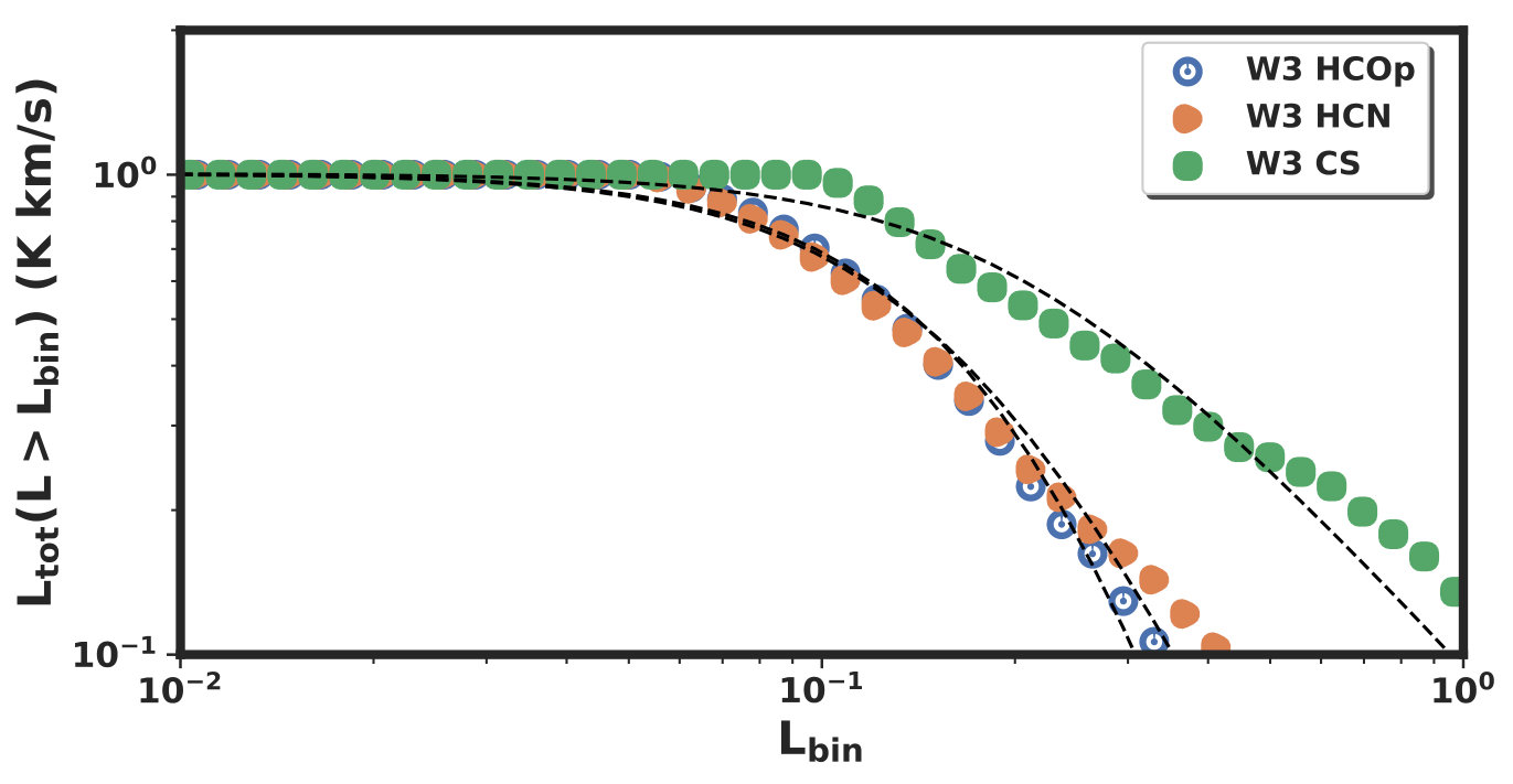 Figure 1
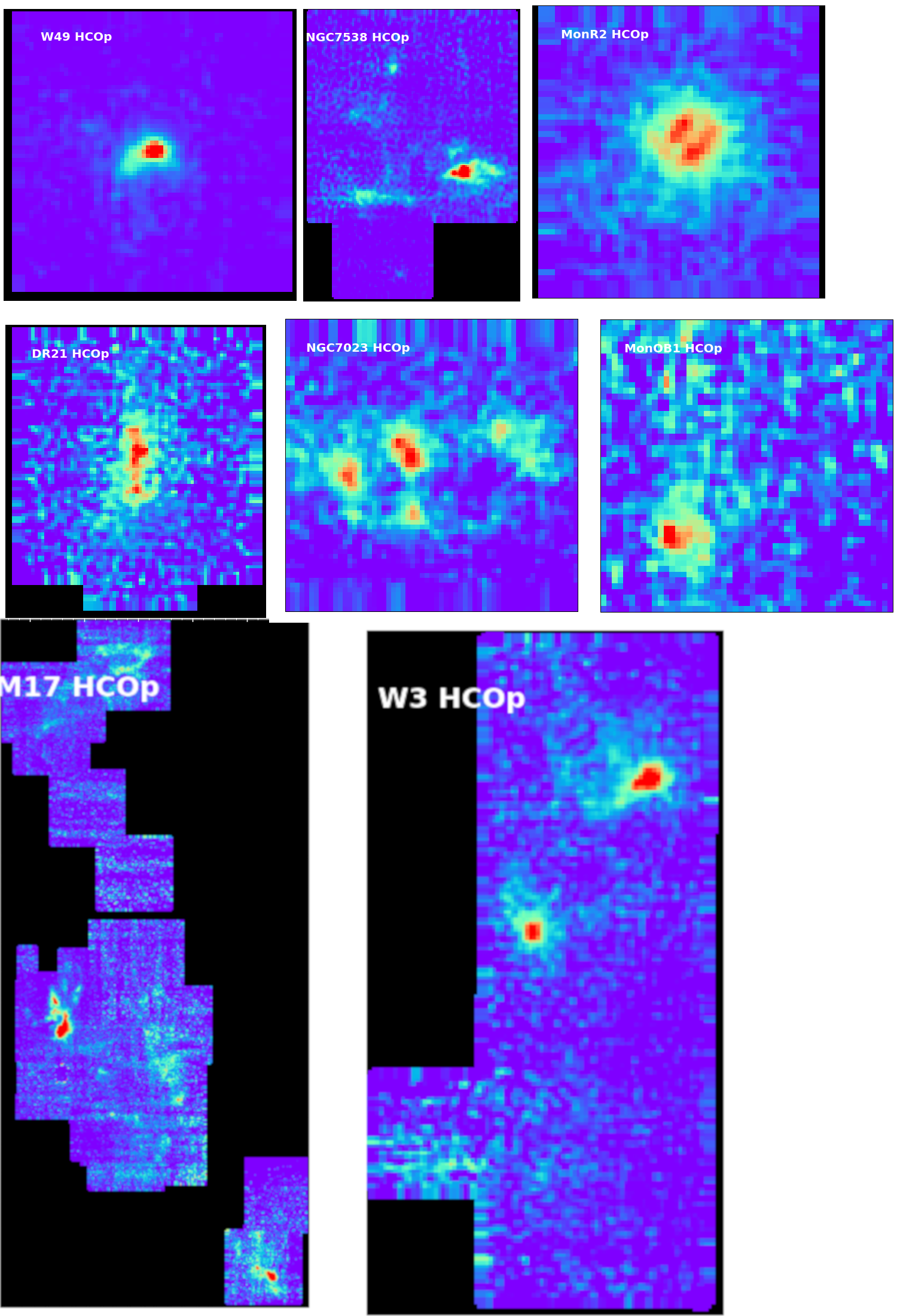 Figure 2
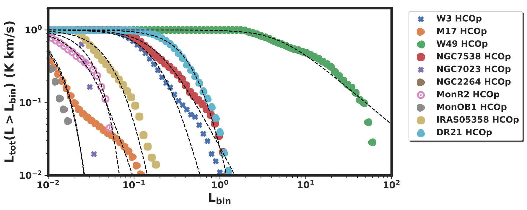 Figure 3
 Figure 4
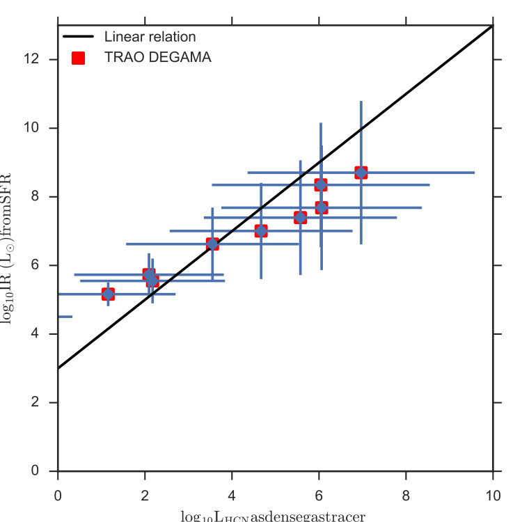 Figure 5
Peer Reviews
No public reviews on file for this paper yet. If you reviewed it on a platform where reviews are public (OpenReview, ICLR, NeurIPS, ICML), you can paste yours below so the community can read it here.
Videos
No videos yet. Explain this paper in a talk, walkthrough, or lecture? Add one.
The dense galactic environments of the Milky Way
Quang Nguyen-Luong1,2,3
Neal Evans4,2
Kee-Tae Kim2
Hyunwoo Kang2 and DEGAMA survey
1IBM Canada, 120 Bloor Street East, Toronto, ON, M4Y 1B7, Canada,
2Korea Astronomy and Space Science Institute, Yuseoung, Daejeon 34055, Korea,
3Visiting researcher at the Graduate School of Natural Sciences, Nagoya City University, Japan
4Department of Astronomy, The University of Texas at Austin, 2515 Speedway, Stop C1400, Austin, TX 78712-1205, USA
email: [email protected]
(2019)
Abstract
Star formation takes place in the dense gas phase, and therefore a simple dense gas and star formation rate relation has been proposed. With the advent of multi-beam receivers, new observations show that the deviation from linear relations is possible. In addition, different dense gas tracers might also change significantly the measurement of dense gas mass and subsequently the relation between star formation rate and dense gas mass. We report the preliminary results the DEnse GAs in MAssive star-forming regions in the Milky Way (DEGAMA) survey that observed the dense gas toward a suit of well-characterized massive star forming regions in the Milky Way. Using the resulting maps of HCO*+* 1–0, HCN 1–0, CS 2–1, we discuss the current understanding of the dense gas phase where star formation takes place.
keywords:
stars: formation, ISM: clouds, ISM: structure, (ISM:) evolution, Galaxy: evolution
††volume: 345††journal: Origins: from the Protosun to the First Steps of Life††editors: Bruce G. Elmegreen, L. Viktor Tóth, Manuel Güdel, eds.
1 Introduction
We perform a survey of DEnse GAs in MAssive star-forming regions in the Milky Way (DEGAMA) survey to study the distribution of dense gas in molecular clouds and its role in forming stars. DEGAMA focusses on a larger sample that is sensitive to all gas above a column density threshold of 1022 cm*-2* with the goal of improving the understanding of how dense gas is formed and the relation between dense gas and star formation. The threshold column density of cm*-2*, which might correspond to a volume density of cm*-3*, is chosen because this gas directly builds massive star forming regions and forms lower mass stars (i.e., [Onishi et al. (1998), Onishi et al. 1998], [André et al. (2010), Andre et al. 2010]).
At the extragalactic scale, we seek to understand the relationship between stellar density and gas density that was put forward by [Thackeray(1948), Thackeray (1948)] and [van den Bergh(1957), Van den Bergh (1957)]), and crystallized in a relationship between the observable surface density of SFR, , and the surface density of gas, , as: by [Schmidt(1959), Schmidt (1959)] and [Kennicutt(1998), Kennicutt (1998)]. However, this relation is not scale-invariant, the power-law indexes depend on the size scales of the objects, as pointed out using the diffuse cloud tracer CO 1–0 and radio continuum luminosity ([nguyen-luong16, Nguyen Luong et al. 2016]). These relationships may behave differently if one considers only dense gas tracers, as was suggested for extragalactic environment ([Wu et al.(2010)Wu, Evans, Shirley, & Knez, Wu et al. 2010], [liu16, Liu et al. 2016]). The linear relationship manifests in the extragalactic environments ([Gao & Solomon (2004), Gao & Solomon 2004]) and in the Milky Way environments ([Lada et al.(2012)Lada, Forbrich, Lombardi, & Alves, Lada et al. 2012]), but significant gaps remain between extragalactic and galactic star formation laws ([Heiderman et al.(2010)Heiderman, Evans, Allen, Huard, & Heyer, Heiderman et al. 2010]). Nevertheless, the linear relationship between dense gas and SFR shows real scatter in excess of observational uncertainties ([Usero et al.(2015)Usero, Leroy, Walter, Schruba, García-Burillo, Sandstrom, Bigiel, Brinks, Kramer, Rosolowsky, Schuster, & de Blok, Usero et al. 2015]), so additional factors are at work beyond a simple “more dense gas gives more star formation” model.
At the extragalactic scale, we seek to understand the relationship between stellar density and gas density that was put forward by [Thackeray(1948), Thackeray (1948)] and [van den Bergh(1957), Van den Bergh (1957)]), and crystallized in a relationship between the observable surface density of SFR, , and the surface density of gas, , as: by [Schmidt(1959), Schmidt (1959)] and [Kennicutt(1998), Kennicutt (1998)]. However, this relation is not scale-invariant, the power-law indexes depend on the size scales of the objects, as pointed out using the diffuse cloud tracer CO 1–0 and radio continuum luminosity ([nguyen-luong16, Nguyen Luong et al. 2016]). These relationships may behave differently if one considers only dense gas tracers, as was suggested for extragalactic environment ([Wu et al.(2010)Wu, Evans, Shirley, & Knez, Wu et al. 2010], [liu16, Liu et al. 2016]). The linear relationship manifests in the extragalactic environments ([Gao & Solomon (2004), Gao & Solomon 2004]) and in the Milky Way environments ([Lada et al.(2012)Lada, Forbrich, Lombardi, & Alves, Lada et al. 2012]), but significant gaps remain between extragalactic and galactic star formation laws ([Heiderman et al.(2010)Heiderman, Evans, Allen, Huard, & Heyer, Heiderman et al. 2010]). Nevertheless, the linear relationship between dense gas and SFR shows real scatter in excess of observational uncertainties ([Usero et al.(2015)Usero, Leroy, Walter, Schruba, García-Burillo, Sandstrom, Bigiel, Brinks, Kramer, Rosolowsky, Schuster, & de Blok, Usero et al. 2015]), so additional factors are at work beyond a simple “more dense gas gives more star formation” model.
With a critical density of cm*-3*, HCO*+* 1–0 (89.188 MHz) and HCN 1–0 (88.631 GHz), and CS 2–1 (97.980 GHz) is suitable to trace the total dense gas component in star forming regions. We observed these lines with the Taeduk Radio Astronomy Observatory (TRAO) telescope 111https://radio.kasi.re.kr/trao/main_trao.php in the DEGAMA survey and report its first results in this paper.
2 Observations
TRAO was established in October 1986 with the 13.7 meter Radio Telescope and recently equipped with the 16 pixels 4x4 SEQUOIA receiver. The 2nd IF modules with the narrow band and the 8 channels with 4 FFT spectrometers allow to observe 2 frequencies simultaneously within the 85–100 or 100–115 GHz bands for all 16 pixels of the receiver. We carried out the DEGAMA mapping observations between December 2016 and December 2017. Observations were done in OTF mode and the native velocity resolution is less than 0.1 km/sec (15 kHz) per channel, and their full spectra bandwidth is 60 MHz. The telescope beam size is \sim 50\mbox{{}^{\prime\prime}} at 100 GHz, and the main-beam efficiency is at 100 GHz.
Our target is a sample of massive star-forming cloud complexes in the Galaxy that present the entire massive star forming sequences from quiescent to active and evolved regions. This sample includes the massive star forming regions that are rather nearby (d kpc), so known star formation rates measurements from direct YSOs counting with Spitzer/WISE or Herschel. The sample includes the following sources that can be categorized in evolutionary stages, from quiescient to more active states: M17, M16, DR21, IRAS05358, W3, MonOB1, NGC7538, NGC2264, W40, NGC7023 , MonR2, and Mon-OB1.
3 Results
From a global perspective, dense gas tracers such as or and SFR tracers such as or are believed to correlate well with each other in log-log space ([Gao & Solomon (2004), Gao & Solomon .2004], [Bussmann et al. (2008), Bussmann et al. 2008], [Wu et al.(2010)Wu, Evans, Shirley, & Knez, Wu et al. 2010]). The relations, however, are not identical for different transitions nor for different dense gas tracers ([Krumholz & Tan(2007), Krumholz & Tan 2007], [Narayanan et al.(2008)Narayanan, Cox, Shirley, Davé, Hernquist, & Walker, Narayanan 2008], [Juneau et al.(2009)Juneau, Narayanan, Moustakas, Shirley, Bussmann, Kennicutt, & Vanden Bout, Juneau et al. 2009]). Moreover, intrinsic variation in this relationship suggests that simple correlations are inadequate for capturing the full range of star formation behavior ([Usero et al.(2015)Usero, Leroy, Walter, Schruba, García-Burillo, Sandstrom, Bigiel, Brinks, Kramer, Rosolowsky, Schuster, & de Blok, Usero et al. 2015]).
We calculate the integrated line luminosity using equation developed in [Solomon & Vanden Bout(2005), Solomon & Vanden Bout (2005)] where
[TABLE]
In DEGAMA survey, integrated line luminosity was derived from a collection of integrated maps of HCO*+* 1–0, HCN 1–0 and CS 2–1. Figure 1 shown an example of only HCO*+* 1–0 maps. The ratio of from DEGAMA survey show that HCO*+* varies from cloud-to-cloud and vary around the average extragalactic ratio of 2 (Figure 2a). It might show that although having similar critical density, HCO*+* and HCN might trace quite different types of dense gas that When plotting on the - plane, there is evidence that Galactic clouds do not follow a simple linear relation as the extragalactic clouds or the scatter is very large (Figure 2b).
Then, we divide the integrated line luminosities into a 100 bins and calculate the cumulative distributions (CDs) of the integrated line luminosities for each bin. The results are plotted as functions of luminosity bin in normalized forms (Figure 3). As the CDs profiles are different for different sources and different tracers, we model them using a Plummer-like function that describes flat plateaux and powerlaw decreasing at higher column density as:
[TABLE]
is the luminosity threshold of each bin, is the total luminosity of the cloud, is where the luminosity profile changes from power-law shape to flat plateau, and is the power-law index of the profile’s section at the high luminosity tail. Figures 3 show that each cloud can be characterized by parameters , , from the profile in Equation 2. This differentiation is potential applicable to differentiate different types of clouds and also its behaviour in different dense gas tracers. We will explore this topic further in the next paper.
The reference list from the paper itself. Each links out to its DOI / PubMed record.
- 1[André et al. (2010)] André, P., Men’shchikov, A., Bontemps, S., et al. 2010, A&A, 518, L 102+
- 2[Bussmann et al. (2008)] Bussmann, R. S., Narayanan, D., Shirley, Y. L., et al. 2008, Ap J, 681, L 73
- 3[Gao & Solomon (2004)] Gao, Y., & Solomon, P. M. 2004, Ap JS, 152, 63
- 4[Heiderman et al.(2010)Heiderman, Evans, Allen, Huard, & Heyer] Heiderman, A., Evans, II, N. J., Allen, L. E., Huard, T., & Heyer, M. 2010, Ap J, 723, 1019
- 5[Hennemann et al. (2010)] Hennemann, M., Motte, F., Bontemps, S., et al. 2010, A&A, 518, L 84+
- 6[Hill et al. (2011)] Hill, T., Motte, F., Didelon, P., et al. 2011, A&A, 533, A 94
- 7[Juneau et al.(2009)Juneau, Narayanan, Moustakas, Shirley, Bussmann, Kennicutt, & Vanden Bout] Juneau, S., Narayanan, D. T., Moustakas, J., et al. 2009, Ap J, 707, 1217
- 8[Kennicutt(1998)] Kennicutt, Jr., R. C. 1998, Ap J, 498, 541