Uniform boundedness and continuity at the Cauchy horizon for linear waves on Reissner-Nordstr\"om-AdS black holes
Christoph Kehle

TL;DR
This paper proves that massive scalar waves on Reissner-Nordström-AdS black holes remain uniformly bounded and continuous at the Cauchy horizon, addressing a key aspect of the Strong Cosmic Censorship Conjecture in AdS spacetimes.
Contribution
It establishes uniform boundedness and continuity of scalar waves at the Cauchy horizon for the first time in the AdS black hole interior setting.
Findings
Scalar waves are uniformly bounded at the Cauchy horizon.
Continuity of waves extends up to the Cauchy horizon.
Results support the Strong Cosmic Censorship Conjecture in AdS contexts.
Abstract
Motivated by the Strong Cosmic Censorship Conjecture for asymptotically AdS spacetimes, we initiate the study of massive scalar waves satisfying on the interior of Anti-de Sitter (AdS) black holes. We prescribe initial data on a spacelike hypersurface of a Reissner--Nordstr\"om--AdS black hole and impose Dirichlet (reflecting) boundary conditions at infinity. It was known previously that such waves only decay at a sharp logarithmic rate (in contrast to a polynomial rate as in the asymptotically flat regime) in the black hole exterior. In view of this slow decay, the question of uniform boundedness in the black hole interior and continuity at the Cauchy horizon has remained up to now open. We answer this question in the affirmative.
Click any figure to enlarge with its caption.
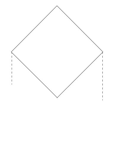 Figure 1
 Figure 2
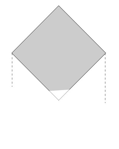 Figure 3
 Figure 4
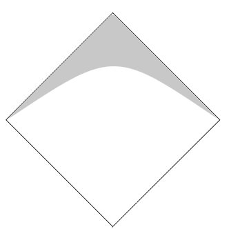 Figure 5
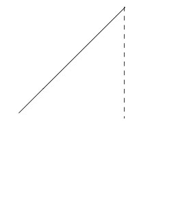 Figure 6
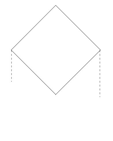 Figure 7
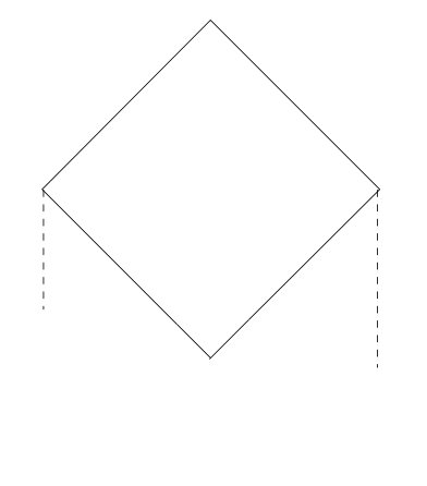 Figure 8
Peer Reviews
No public reviews on file for this paper yet. If you reviewed it on a platform where reviews are public (OpenReview, ICLR, NeurIPS, ICML), you can paste yours below so the community can read it here.
Videos
No videos yet. Explain this paper in a talk, walkthrough, or lecture? Add one.
Uniform boundedness and continuity at the Cauchy horizon
for linear waves on Reissner–Nordström–AdS black holes
Christoph Kehle [email protected] Department of Pure Mathematics and Mathematical Statistics,
University of Cambridge, Wilberforce Road, Cambridge CB3 0WB, United Kingdom
(July 22, 2019)
Abstract
Motivated by the Strong Cosmic Censorship Conjecture for asymptotically AdS spacetimes, we initiate the study of massive scalar waves satisfying on the interior of Anti-de Sitter (AdS) black holes. We prescribe initial data on a spacelike hypersurface of a Reissner–Nordström–AdS black hole and impose Dirichlet (reflecting) boundary conditions at infinity. It was known previously that such waves only decay at a sharp logarithmic rate (in contrast to a polynomial rate as in the asymptotically flat regime) in the black hole exterior. In view of this slow decay, the question of uniform boundedness in the black hole interior and continuity at the Cauchy horizon has remained up to now open. We answer this question in the affirmative.
Contents
1 Introduction
We initiate the study of (massive) linear waves satisfying
[TABLE]
on the interior of asymptotically Anti-de Sitter (AdS) black holes . In the context of asymptotically AdS spacetimes it is natural to consider (possibly negative) mass parameters satisfying the Breitenlohner–Freedman [6] bound , where is the cosmological constant of the underlying spacetime. In particular, this covers the conformally invariant operator with . We will consider Reissner–Nordström–AdS (RN–AdS) black holes [7] which can be viewed as the simplest model in the context of the question of stability of the Cauchy horizon. These spacetimes are spherically symmetric solutions of the Einstein equations
[TABLE]
coupled to the Maxwell equations via the energy momentum tensor . Our main result 1 (see Theorem 3.1 in Section 3 for its precise formulation) is the statement of uniform boundedness in the black hole interior and continuity at the Cauchy horizon of solutions to (1.1) arising from initial data on a spacelike hypersurface on RN–AdS. We moreover assume Dirichlet (reflecting) boundary conditions at infinity. Our result is surprising because in contrast to black hole backgrounds with non-negative cosmological constants (), the decay of in the exterior region for asymptotically AdS black holes () is only logarithmic as shown by Holzegel–Smulevici [39] (cf. polynomial [59, 19, 1] () and exponential [5, 25] ()). Indeed, the logarithmic decay is too slow to adapt the mechanism exploited in previous studies of black hole interiors [14, 26, 17]. The proof of our main theorem will now follow a new approach, combining physical space estimates with Fourier based estimates exploited in the scattering theory developed in [43].
In the rest of the introduction we will give some background on the problem and formulate our main result 1.
The Cauchy horizon and the Strong Cosmic Censorship Conjecture
The main motivation for studying linear waves on black hole interiors is to shed light on one of the most fundamental puzzles in general relativity: The Kerr(–de Sitter or –Anti-de Sitter) and Reissner–Nordström (–de Sitter or –Anti-de Sitter) black holes share the property that in addition to the event horizon , they hide another horizon, the so-called Cauchy horizon , in their interiors. 111More precisely, this holds true for subextremal and non-trivially rotating(charged) Kerr(Reissner–Nordström) black holes which we will assume for the rest of the paper, unless explicitly stated otherwise. This Cauchy horizon defines the boundary beyond which initial data on a spacelike hypersurface (together with boundary conditions at infinity in the asymptotically AdS case) no longer uniquely determine the spacetime as a solution of (EE). In particular, these spacetimes admit infinitely many smooth extensions beyond their Cauchy horizons solving (EE). This severe violation of determinism is conjectured to be an artifact of the high degree of symmetry in those explicit spacetimes and generically, due to blue-shift instabilities, it is expected that a singularity ought to form at or before the Cauchy horizon. This is known as the Strong Cosmic Censorship Conjecture (SCC) [57, 9]. A full resolution of the SCC conjecture would also include a precise description of the breakdown of regularity at or before the Cauchy horizon.
We first present the formulation of SCC (see [9, 17]), which can be seen as the strongest inextendibility statement in this context.
Conjecture 1** ( formulation of strong cosmic censorship).**
For generic compact or asymptotically flat (asymptotically Anti-de Sitter) vacuum initial data, the maximal Cauchy development of (EE) is inextendible as a Lorentzian manifold with (continuous) metric.
Surprisingly, the formulation (1) was recently proved to be false for both cases and (see discussion later, [17]). However, the following weaker, yet well-motivated, formulation introduced by Christodoulou in [9] is still expected to hold true (at least) in the asymptotically flat case ().
Conjecture 2** (Christodoulou’s re-formulation of strong cosmic censorship).**
For generic asymptotically flat vacuum initial data, the maximal Cauchy development of (EE) is inextendible as a Lorentzian manifold with (continuous) metric and locally square integrable Christoffel symbols.
In order to gain insight about SCC, the most naive approach (often referred to as “poor man’s linearization”) is to study solutions of (1.1) with on a fixed explicit black hole spacetime (e.g. Kerr or Reissner–Nordström). This can be considered as the most naive toy model for (EE) with initial data close to Kerr or Reissner–Nordström data, for which many features of (EE) including the non-linear terms and the tensorial structure are neglected; see the pioneering works for asymptotically flat () black holes [60, 48, 49, 8]. Under the identification and , where is a solution to (1.1), 1 corresponds to a failure of to be continuous () at the Cauchy horizon. Similarly, 2 corresponds to a failure of to lie in at the Cauchy horizon.
The state of the art for and
The definitive disproof [17] of 1 was preceded by corresponding results on the level of (1.1).
Linear level for
In the asymptotically flat case () it was shown in [26, 27] (see also [34]) that solutions of (1.1) with arising from data on a spacelike hypersurface remain continuous and uniformly bounded (no blow-up) at the Cauchy horizon of general subextremal Kerr or Reissner–Nordström black hole interiors. (For the extremal case see [30, 31].) The key method for the proof is to use the polynomial decay on the event horizon proved in [19] (with rate and ) and propagate it into the interior. The boundedness and continuity of at the Cauchy horizon was then concluded from red-shift estimates, energy estimates associated to the novel vector field
[TABLE]
and commuting with angular momentum operators followed by Sobolev embeddings. Here are Eddington–Finkelstein-type null coordinates in the interior.
Besides the above boundedness, it was proved that the (non-degenerate) local energy at the Cauchy horizon blows up for a generic set of solutions in Reissner–Nordström [44] and Kerr [20] black holes. (Note that this blow-up is compatible with the finiteness of the flux associated to (1.2) because and degenerate at the Cauchy horizons and , respectively.) A similar blow-up behavior was obtained for Kerr in [47] assuming lower bounds on the energy decay rate of a solution along the event horizon. These results support 2 at least on the level of (1.1).
Another type of result that has been shown in [43] is a finite energy scattering theory for solutions of (1.1) (with ) from the event horizon to the Cauchy horizon in the interior of Reissner–Nordström black holes. In this scattering theory a linear isomorphism between the degenerate energy spaces (associated to the Killing field ) corresponding to the event and Cauchy horizon was established. The question reduced to obtaining uniform control over transmission and reflection coefficients and corresponding to fixed frequency solutions. Intuitively, for a purely incoming wave at the event horizon , the transmission and reflection coefficients correspond to the amount of -energy scattered to and , respectively. Indeed, the theory also carries over to and except for the frequency. This will turn out to be important for the present paper.
Linear level for
For Kerr(and Reissner–Nordström)–de Sitter () it was shown in [35] that solutions of (1.1) (with ) also remain bounded up to and including the Cauchy horizon. Note that in both cases, and , the proofs rely crucially on quantitative decay along the event horizon (polynomial for and exponential for ).
On the other hand the exponential convergence on the event horizon of a Kerr–de Sitter black hole is in direct competition with the exponential blue-shift instability and the question of local energy blow-up at the Cauchy horizon for (1.1) is more subtle, see the conjecture in [15] and the more recent [21, 23, 22].
Nonlinear level for and
Now we turn to the full nonlinear problem for (EE). As mentioned before, for the Einstein vacuum equations Dafermos–Luk showed that the Kerr Cauchy horizon is stable [17], i.e. the spacetime is extendible as a Lorentzian manifold. Note that this definitively falsifies 1 for (subject only to the completion of a proof of the nonlinear stability of the Kerr exterior). In principle, their proof of extendibility also applies to the interior of Kerr–de Sitter black holes, where the exterior has been proved to be stable for slowly rotating Kerr–de Sitter black holes [36], thus falsifying 1 for .
Nonlinear inextendibility results at the Cauchy horizon have been proved only in spherical symmetry: Coupling the Einstein equation (EE) to a Maxwell–Scalar field system, it is proved in [14] that the Cauchy horizon is stable, yet unstable [45, 46, 14] for a generic set of spherically symmetric initial data. See also the pioneering work in [58, 56]. This shows the formulation of SCC (but not yet 2) in spherical symmetry. See [12, 13] for work in the case. The question of any type of nonlinear instability of the Cauchy horizon without symmetry assumptions and the validity of 2 (even restricted to a neighborhood of Kerr) have yet to be understood.
Linear waves and SCC for asymptotically AdS black holes
The situation is changed radically if one considers asymptotically Anti-de Sitter () spacetimes.
Due to the timelike nature of null infinity , see for example Fig. 1, these spacetimes are not globally hyperbolic. For well-posedness of (EE) and (1.1) it is required to impose also boundary conditions at infinity. The most natural conditions are Dirichlet (reflecting) boundary conditions, see [29]. Before we address the question of stability of the Cauchy horizon, it is essential to understand the behavior in the exterior region of Kerr–AdS or Reissner–Nordström–AdS.
Logarithmic decay for linear waves on the exterior of Kerr–AdS and Reissner–Nordström–AdS
For the massive linear wave equation (1.1) on Kerr–AdS and Reissner–Nordström–AdS, Holzegel–Smulevici showed in [39] stability in the exterior region. Indeed, they proved that solutions decay at least at logarithmic rate towards (cf. polynomial () and exponential ()) assuming the Hawking–Reall [33] bound222Note that otherwise exponentially growing mode solutions can be constructed as shown in [24]. and the Breitenlohner–Freedman [6] bound . Moreover, they showed that solutions of (1.1) with fixed angular momentum actually decay exponentially on the exterior of Reissner–Nordström–AdS. (This is in contrast to the asymptotically flat case, in which fixed angular momentum solutions of (1.1) decay polynomially on the exterior of Reissner–Nordström.) However, their main insight was that a suitable infinite sum of such rapidly decaying fixed angular momentum solutions, possessing finite energy in some weighted norm, indeed achieves the logarithmic decay rate [41]. This is due to the presence of stable trapping. Note that this sharpness can also be concluded from later work showing the existence of quasinormal modes converging to the real axis at an exponential rate as the real part of the frequency and angular momentum tend to infinity [64, 32]. (For some asymptotically flat five dimensional black holes a similar inverse logarithmic lower bound was shown in [2].)
Strong Cosmic Censorship for AdS black holes
With the logarithmic decay on the exterior in hand, we turn to the question of the stability of the Cauchy horizon. Indeed, the logarithmic decay rate on the exterior is too slow to follow the methods involving the red-shift vector field and the vector field as in (1.2) (see discussion before) to prove uniform boundedness and (continuous) extendibility at the Cauchy horizon of solutions to (1.1). More specifically, after propagating the logarithmic decay through the red-shift region, the energy flux associated to is infinite on a hypersurface in the black hole interior due to the slow logarithmic decay towards . Thus, the question of whether to expect the validity of 1 for asymptotically AdS black holes appears to be completely open. (See also the paragraph in the end of the introduction discussion a possible nonlinear instability in the exterior.)
The present paper is an attempt to shed some first light on SCC in the asymptotically AdS case: We will show (1) that, despite the slow decay on the exterior, boundedness in the interior and continuous extendibility to the Cauchy horizon still holds for solutions of (1.1) on Reissner–Nordström–AdS black holes. The additional phenomenon which we exploit to prove boundedness is that the trapped frequencies responsible for slow decay have high energy with respect to the vector field and can be bounded using the scattering theory developed in [43]. Thus, for Reissner–Nordström–AdS, the analog of 1 is false on the linear level, just as in the cases. See however our remarks on Kerr–AdS later in the introduction.
The massive linear wave equation on Reissner–Nordström–AdS
As mentioned above, we will consider the massive linear wave equation
[TABLE]
for AdS radius on a fixed subextremal Reissner–Nordström–AdS black hole with mass parameter and charge parameter . Moreover, we assume the so-called Breitenlohner–Freedman bound [6] for the Klein–Gordon mass parameter , which includes the conformally invariant case . This bound is required to obtain well-posedness [38, 63, 62] of (1.3).
Recall from the discussion above that solutions with fixed angular momentum actually decay exponentially in the exterior region. For such solutions with fixed , uniform boundedness with upper bound in the interior and continuity at the Cauchy horizon can be shown using the methods involving the vector field as in (1.2). Note however that this does not imply that a general solution remains bounded in the interior as the constant is not summable: as . Note in particular that, as a result of this, one cannot study the new non-trivial aspect of this problem restricted to spherical symmetry. (Nevertheless, see [3] for a discussion of the Ori model for RN–AdS black holes.)
Main theorem: Uniform boundedness and continuity at the Cauchy horizon
We now state a rough version of our main result. See Theorem 3.1 for the precise statement.
Theorem 1** (Rough version of Theorem 3.1).**
Let be a solution to (1.3) arising from smooth and compactly supported initial data posed on a spacelike hypersurface as depicted in Fig. 1. Then, remains uniformly bounded in the black hole interior
[TABLE]
where is constant depending on the parameters , the choice of and on some higher order Sobolev norm of the initial data . Moreover, can be extended continuously across the Cauchy horizon.
As we have explained above, the main difficulty compared to the asymptotically flat case, where the analysis was carried out entirely in physical space and requires inverse polynomial decay in the exterior [26], is the slow decay of along the event horizon. Our strategy is to decompose the solution in a low and high frequency part with respect to the Killing field and treat each term separately.
For the low frequency part , we will show a superpolynomial decay rate in the exterior, see already 4.8. For this part we also use integrated energy decay estimates for bounded angular momenta established in [39]. This superpolynomial decay in the exterior is sufficient so as to follow the method of [26] with vector fields of the form (1.2) to show boundedness and continuity at the Cauchy horizon, up to the additional difficulty caused by the fact that we allow a possibly negative Klein–Gordon mass parameter. The violation of the dominant energy condition due to the presence of a negative mass term can be overcome with twisted derivatives [63, 42], which provide a useful framework to replace Hardy inequalities for the lower order terms in this context.
For the high frequency part , which is exposed to stable trapping and does in general only decay at a sharp logarithmic rate in the exterior, the key ingredient is the scattering theory developed in [43] (see discussion above). More specifically, the uniform bounds for the transmission and reflections coefficients and for proved in [43] turn out to be useful for the high frequency part . These bounds allow us to control at the Cauchy horizon by the -energy norm on the event horizon commuted with angular derivatives. The -energy flux on the event horizon is in turn bounded from initial data by a simple application of the -energy identity in the exterior. In particular, no quantitative decay along the event horizon is used for the high frequency part . This is what allows us to overcome the problem of slow logarithmic decay.
Outlook on Kerr–AdS
We strongly believe that our arguments also apply to axially symmetric solutions of (1.3) on a Kerr–AdS black hole. For general non-axisymmetric solutions, however, the question of uniform boundedness and continuity at the Cauchy horizon is less clear. Indeed, specific high frequency solutions which decay at a logarithmic decay rate can be considered as “low frequency” solutions when frequency is measured with respect to the Killing generator of the Cauchy horizon. In fact, it might well be the case that for solutions of (1.3) on Kerr–AdS there is blow-up at the Cauchy horizon, supporting the validity of 1 after all in this context!
Instability of asymptotically AdS spacetimes?
Turning to the fully nonlinear dynamics, there is another scenario which could happen. Recall that Minkowski space () and de Sitter space () have been proved to be nonlinearly stable [28, 10]. Anti-de Sitter space (), however, is expected to be nonlinearly unstable with Dirichlet conditions imposed at infinity. This was recently proved in [51, 50, 53, 52] for appropriate matter models. See also the original conjecture in [16] and the numerical results in [4]. Similarly, for Kerr–AdS (or Reissner–Nordström–AdS), the slow logarithmic decay on the linear level proved in [41] could in fact give rise to nonlinear instabilities in the exterior.333Note that in contrast, nonlinear stability for spherically symmetric perturbations of Schwarzschild–AdS was shown for Einstein–Klein–Gordon systems [40]. If indeed the exterior of Kerr–AdS was nonlinearly unstable, linear analysis like that in the present paper would be manifestly inadequate and the question of the validity of Strong Cosmic Censorship would be thrown even more open! Refer to the introduction of [17] for a more elaborate discussion.
Outline
This paper is organized as follows. In Section 2 we set up the spacetime and summarize relevant previous work. In Section 3 we state and prove our main result Theorem 3.1. Parts of the proof require a separate analysis which are treated in Section 4 and Section 5.
Acknowledgment
The author would like to express his gratitude to Mihalis Dafermos and Yakov Shlapentokh-Rothman for many valuable discussions and helpful remarks. The author thanks John Anderson, Anne Franzen, Dejan Gajic, Jonathan Luk, Georgios Moschidis, Federico Pasqualotto, Igor Rodnianski and Claude Warnick. The author also thanks two anonymous referees for their helpful comments. This work was supported by the EPSRC grant EP/L016516/1. The author thanks Princeton University for hosting him as a VSRC.
2 Preliminaries
We start by setting up the Reissner–Nordström–AdS spacetime (see [7]) and defining relevant norms and energies. We will also introduce useful coordinate systems.
2.1 The Reissner–Nordström–AdS black hole
We are ultimately interested in the behavior of solutions to (1.3) to the future of a spacelike hypersurface as depicted in Fig. 1. For technical reasons (Fourier space decompositions are non-local operations) we will however construct also parts to the past of . In the following will define the spacetime pictured in Fig. 2.
2.1.1 Construction of the spacetime
First, for black hole parameters define the polynomial
[TABLE]
and define the non-degenerate set
[TABLE]
Note that defines black hole parameters in the subextremal range. From now on, we will consider fixed parameters , where
[TABLE]
Note that is the mass parameter, the charge parameter of the black hole and is the Anti-de Sitter radius. For this specific choice of parameters we will also write and denote by the positive roots of .
Now, let the two exterior regions , and the black hole region be smooth four dimensional manifolds diffeomorphic to . On and we introduce global444Up to the known degeneracy of spherical coordinates at the poles of the sphere. coordinate charts:
[TABLE]
If it is clear from the context which coordinates are being used, we will omit their subscripts throughout the paper. Again, on the manifolds and we define—using the coordinates on each of the patches—the Reissner–Nordström–Anti-de Sitter metric
[TABLE]
On each of and , we define time orientations using the vector field on , on and on .
We will also define the tortoise coordinate by
[TABLE]
in , and independently. This defines up to an unimportant constant. Then, in each of the regions , and , we define null coordinates by
[TABLE]
where for example for the coordinate on , we will use the notation and analogously for the other regions. Note that throughout the paper we will use the notation ′ for derivatives .
Patching the regions and together
Now, we patch the regions , and together. We begin by attaching the future (resp. past) event horizon (resp. ) to by formally555This can be made rigorous using ingoing Eddington–Finkelstein coordinates () adapted to the event horizon. Since this is well-known, we avoid introducing yet another coordinate system. setting
[TABLE]
Similarly, we attach and to . In the coordinates associated to we make the identifications and . Then, we attach the Cauchy horizon and to .
Finally, we attach the past (resp. future) bifurcation sphere (resp. ) to as
[TABLE]
We shall also set . Note that all horizons , and are diffeomorphic to and the past (future) bifurcation sphere () is diffeomorphic to . Moreover, we identify with and also with . The resulting manifold will be called . Note that, extends to a smooth Lorentzian metric on which we will call and in particular, is a time oriented smooth Lorentzian manifold with corners. We illustrate the constructed spacetime as a Penrose diagram in Fig. 2. Note that the vector field defined on , and , respectively, extends to a smooth Killing field on , which we will from now on call . Moreover, the standard angular momentum operators for , the generators of defined as
[TABLE]
are Killing vector fields. It shall be noted that for are spacelike everywhere, whereas is future-directed timelike on , spacelike on and past-directed timelike on . Moreover, is future-directed null on , past-directed null on and vanishes on . Finally, note that one can attach conformal timelike boundaries and corresponding to and , respectively.666Note that and are not contained in .
2.1.2 Initial hypersurface
We will impose initial data on a spacelike hypersurface to be made precise in the following. Note that we can choose for convenience that the spacelike hypersurface lies to the future of the past bifurcation sphere . Indeed, by general theory (an energy estimate in a compact region) this can be assumed without loss of generality [18]. More precisely, let be a 3 dimensional connected, complete and spherically symmetric spacelike hypersurface extending to the conformal infinity . Moreover, assume that .
A possible choice of is denoted in Fig. 3. We are ultimately interested in the shaded region to the future of . For the rest of the paper, we will consider such a to be fixed.
2.2 Conventions
With for and we mean that there exists a constant with . If depends on an additional parameter, say , we will write . We also use for some if there exist constants with . We shall also make use of the standard Landau notation and [55]. To be more precise, let be a point set (e.g. ) with limit point . As in , means holds in a fixed neighborhood of . We write if the constant depends on an additional parameter . For the standard volume form in spherical coordinates on the sphere we will use the notation . Finally, let the Japanese symbol be defined as for .
2.3 Norms and Energies
We are interested in solutions to the massive wave equation (1.3) associated to the metric on a subextremal Reissner–Nordström AdS black hole with black hole parameters as in (2.3). In view of the timelike boundaries and , we need to specify boundary conditions on and in addition to prescribing data on the spacelike hypersurface , cf. Fig. 3. We will use Dirichlet (reflecting) boundary conditions which can be viewed as the most natural conditions in the context of stability of the Cauchy horizon. In principle, however, in view of [63], we could also use more general boundary conditions like Neumann or Robin conditions. We will now introduce an appropriate foliation and norms in order to state the well-posedness statement in Section 2.4.
We will foliate with spacelike hypersurfaces. To do so, we let be a smooth future-directed causal vector field on with the properties that
[TABLE]
and that is a future-directed timelike vector field on . Now, define the leaves
[TABLE]
where is the flow generated by and is its affine parameter. We have illustrated some leaves in Fig. 4.
2.3.1 Further coordinates in the exterior region
In the region , we moreover define a global (up to the well-known degeneracy on ) coordinate system , where is the affine parameter of the flow generated by . Note that on we have such that and . Similarly, we can define such a coordinate system on .
2.3.2 Norms on hypersurfaces
By construction intersects , and . We will now define norms on which are adaptations of the norms introduced in [38]. We define
[TABLE]
and
[TABLE]
where each of the terms appearing in (2.12) will be defined in the following.
Norms in the interior region
We begin by defining the first term in (2.12). We define as the standard Sobolev norm of order on the Riemannian manifold .
Norms in the exterior region
Due to the symmetry of the regions and , we will only define the norms on in the following. The norms on are be constructed analogously. We use the coordinates in to define the norms
[TABLE]
and similarly for higher order norms. Here and in the following we denote with and the induced covariant derivative and the induced metric, respectively, on spheres of constant (). We will also use the notation . Now having defined (2.12), we will define energies in the following.
2.3.3 Energies on hypersurfaces
We set
[TABLE]
for , where all terms in (2.14) will be defined in the following.
Energies in the interior region
In the interior region we are not concerned with -weights and define the energies as
[TABLE]
Energies in the exterior region
To define the energies in the exterior region, it is convenient to start with defining the following energy densities
[TABLE]
and their integrals as
[TABLE]
for . Note that we will write for the analogous energy restricted to .
Also remark the following relation between the norms and energies defined above
[TABLE]
2.4 Well-posedness and mixed boundary value Cauchy problem
Having set up the spacetime and the norms, we will restate the well-posedness result for (1.3) as a mixed boundary value-Cauchy problem. For asymptotically AdS spacetimes, well-posedness was first proved in [38].
Theorem 2.1** ([38]).**
Let the Reissner–Nordström–AdS parameters and the Klein–Gordon mass be as in (2.3). Let initial data be prescribed on the spacelike hypersurface and impose Dirichlet (reflecting) boundary conditions on .
Then, there exists a smooth solution of (1.3) such that , . The solution is also unique in the class .
Remark 2.2**.**
The well-posedness statement in Theorem 2.1 holds true for a more general class of initial data, called a initial data triplet which give rise to a solution in , see [38].
2.5 Energy identities and estimates
In order to prove energy estimates, it turns out to be useful to introduce two types of energy-momentum tensors. Besides the standard energy-momentum tensor associated to (1.3), a suitable twisted energy-momentum tensor plays an important role in our estimates. Indeed, due to the negative mass term, the standard energy-momentum tensor does not satisfy the dominant energy condition. However, the dominant energy condition can be restored for the twisted energy-momentum tensor introduced in [6, 63]. In particular, these twisted energies will be used in the interior region, whereas in the exterior region we will work with the standard energy-momentum tensor. We will first review the energy estimates in the exterior.
2.5.1 Energy estimates in the exterior region
Energy-momentum tensor
For a smooth function we define
[TABLE]
For a smooth vector field we also define
[TABLE]
where is the deformation tensor. The term is often referred to as the “bulk term” and satisfies
[TABLE]
if is a solution to (1.3). Note that if is Killing, then vanishes. More generally, integrating (2.20) one obtains an energy identity relating boundary and bulk terms. For more details about the energy-momentum tensor and its usage for standard energy estimates we refer to [18].
Boundedness and decay in the exterior region
In the exterior regions and we have energy decay and boundedness results which have been proved in [38, 37, 39, 41]777Strictly speaking, in [39] this has been only explicitly proved for Kerr–AdS which includes Schwarzschild–AdS. However, the same proof as for Schwarzschild–AdS works completely analogously for Reissner–Nordström–AdS and we shall not repeat these arguments here.. To state them we make the following choice of volume forms and normals on the event horizon. We set and and similarly for . Moreover, we denote by the induced volume form on the spacelike hypersurface and by its future-directed unit normal. We summarize these energy identities and estimates in the following.
Proposition 2.3** ([38]).**
A solution to (1.3) arising from smooth and compactly supported data on as in Theorem 2.1 satisfies
[TABLE]
where and . The analogous energy identity holds in . In particular, (2.21) shows that the -energy flux through vanishes.
Moreover, the -energy flux through the event horizon is bounded by initial data
[TABLE]
Finally, note that
[TABLE]
Remark that (2.23) follows from a Hardy inequality (see [37, Equation (50)]) which is used to absorb the (possibly) negative contribution from the Klein–Gordon mass term.
Theorem 2.4** ([41, Theorem 1.1], [39, Section 12]).**
A solution to (1.3) arising from smooth and compactly supported data on as in Theorem 2.1 satisfies
[TABLE]
and similarly for higher order norms. Moreover, we have the energy decay statements
[TABLE]
for and the pointwise decay
[TABLE]
for in the exterior region and similarly in . Moreover, just like for Schwarzschild–AdS (cf. [39]), fixed angular frequencies decay exponentially. More precisely, let denote the spherical harmonics and let be a solution to (1.3) arising from smooth and compactly supported data on . If there exists an with for , then
[TABLE]
for and a constant only depending on the parameters .
Remark 2.5**.**
Note that (2.28) also implies pointwise exponential decay for (assuming for ) and all higher derivatives of using standard techniques like commuting with and , elliptic estimates as well as applying a Sobolev embedding. Moreover, the previous estimates above also hold true for a the more general class of solutions . See [38] or [39, Theorem 4.1] for more details.
Remark 2.6**.**
The previous decay estimates have only been stated to the future of in the region , nevertheless, they also hold in . Moreover, they also hold true to the past of for an appropriate foliation for which the leaves intersect and , and are transported along the flow of for and along the flow of for .
We now turn to the energy estimates in the interior region .
2.5.2 Energy estimates in the interior region
Twisted energy-momentum tensor
We begin by defining twisted derivatives.
Definition 2.7** (Twisted derivative).**
For a smooth and nowhere vanishing function we define the twisted derivative
[TABLE]
and its formal adjoint
[TABLE]
We shall refer to as the twisting function.
Remark 2.8**.**
Note that we can rewrite the Klein–Gordon equation (1.3) in terms of the twisted derivatives as
[TABLE]
where the potential is given by
[TABLE]
Now, we also associate a twisted energy-momentum tensor to the twisted derivatives.
Definition 2.9** (Twisted energy-momentum tensor).**
Let be smooth and nowhere vanishing and as defined in Definition 2.7. We define the twisted energy-momentum tensor associated to (1.3) and as
[TABLE]
where is as in (2.32) and is any smooth function.
We will now compute the divergence of the twisted energy-momentum tensor.
Proposition 2.10** ([42, Proposition 3]).**
Let be a smooth function and be a smooth nowhere vanishing twisting function. Then,
[TABLE]
where
[TABLE]
Now, assume that moreover satisfies (1.3) and is a smooth vector field. Set
[TABLE]
Then,
[TABLE]
Finally, note that if the twisting function associated to is chosen such that , then satisfies the dominant energy condition, i.e. if is a future pointing causal vector field, then so is .
We will make use of the twisted energy-momentum tensor in the interior region for which we use null coordinates introduced in Section 2.1. For the rest of the subsection we will drop the index . Then, setting
[TABLE]
where , we write the metric in the interior region as
[TABLE]
Note that in the interior we have and . In A.1 in the appendix we have written out the components of the twisted energy-momentum tensor, the twisted 1-jets and the twisted bulk term in null components. We will use the notation , for null cones and for spacelike hypersurfaces in the interior. Furthermore, we set (in mild abuse of notation)
[TABLE]
and analogously for and . We will also make use of the following notation. For any we set
[TABLE]
and for hypersurfaces with constant we denote as their normals.888For null hypersurfaces there does not exist a unit norm normal vector, however, for a fixed volume form, there exists a canonical normal vector which we will choose here. Our choice of volume forms and the corresponding normals can be found in Section A.1.
Twisted red-shift vector field
Proposition 2.11**.**
There exist a , a constant , a nowhere vanishing smooth function associated to the twisted energy momentum tensor and a future directed timelike vector field such that
[TABLE]
for and any smooth solution to (1.3).
Proof.
This is proven in Section A.2. ∎
We will now prove the main estimate which we will use in the red-shift region in the interior.
Proposition 2.12**.**
Let be a smooth solution to (1.3) and let . Then, for any we obtain
[TABLE]
Proof.
We apply the energy identity (spacetime integral of (2.37)) in the region to obtain
[TABLE]
Finally, the claim follows from 2.11. ∎
Twisted no-shift vector field
In this region we propagate estimates towards from the red-shift region to the blue-shift region using a invariant vector field and a -independent twisting function . Take fixed from 2.11 and let be close to . We will use the no-shift vector field in two different parts of the paper: First, we will use it in the proof of A.2 in the appendix in order to prove well-definedness of the Fourier projections. In this case we will choose in principle arbitrarily close to . The estimate degenerates as we take , however for the purpose of A.2 such an estimate is sufficient. Our second application of the no-shift vector field is to propagate decay of the low-frequency part in the interior (see already Section 4.2). Here, we will take only depending on the black hole parameters as determined in 4.16.
In either case, we will choose
[TABLE]
as our vector field. (Indeed, any future directed and invariant vector field would work.) We define our twisting function as
[TABLE]
for some large enough such that
[TABLE]
uniformly in . In particular, since is bounded away from , we have
[TABLE]
for a smooth function . Our main estimate in the no-shift region is
Proposition 2.13**.**
Let be a smooth solution to (1.3) and . Then for any we have
[TABLE]
where we remark that
Proof.
We apply the energy identity (spacetime integral of (2.37)) with (cf. (2.45)) and as in (2.46) in the region . The choice of guarantees the twisted dominated energy condition for the twisted energy-momentum tensor. Together with the coarea formula as well as the facts that is compact and is invariant, we conclude
[TABLE]
for a constant . Similarly, after setting
[TABLE]
for , we also have
[TABLE]
for a constant . An application of Grönwall’s inequality yields
[TABLE]
which implies the result. ∎
We will use an additional vector field in the interior in the blue-shift region . We will however only define it later in the paper in Section 4.2.3 when we actually use it to propagate estimates for the low-frequency part all the way to the Cauchy horizon.
Notation**.**
In the main part of the paper we will makes use of the Fourier transform and convolution associated to the coordinate in coordinates as in (2.4). We denote as the Fourier transform (and as its inverse) defined as
[TABLE]
in the coordinates of and , respectively. Here, we assume that is (at least) a tempered distribution and (2.54), in general, is to be understood in the distributional sense. Moreover, the convolution associated to the coordinate is defined as
[TABLE]
where we again assume that is a tempered distribution and is a Schwartz function. Here, (2.55), in general, is to be understood in the distributional sense.
3 Main theorem and frequency decomposition
Now, we are in the position to state our main result
Theorem 3.1**.**
Let the Reissner–Nordström–AdS parameters and the Klein–Gordon mass be as in (2.3). Let be a solution to (1.3) arising from smooth and compactly supported initial data on with Dirichlet (reflecting) boundary conditions imposed at and (cf. Theorem 2.1). Then, is uniformly bounded in the interior region satisfying
[TABLE]
where is defined as
[TABLE]
Moreover, extends continuously to the Cauchy horizon, i.e. .
Remark 3.2**.**
The data term in (3.2) can be controlled by the initial data such that (3.1) can be written in terms of initial data as
[TABLE]
for a constant only depending on the parameters and the choice of initial hypersurface .
Remark 3.3**.**
Theorem 3.1* can be extended to a more general class of initial data using standard density arguments. In the context of uniform boundedness and continuity at the Cauchy horizon, it is enough to consider smooth and localized initial data. Nevertheless, note that for more general initial data in appropriate Sobolev spaces, already well-posedness becomes more delicate [38].*
Proof of Theorem 3.1.
We split up the proof in four steps, where Step 3 and Step 4 are the main parts relying on Section 4 and Section 5.
Step 1: Decomposition into low and high frequencies
Let
[TABLE]
be as in the assumption of Theorem 3.1. Now, in , and in , define the low frequency part and the high frequency part as
[TABLE]
where
[TABLE]
From A.4 in the appendix we know that the low and high frequency parts and in (3.5) are well-defined and and extend to smooth solutions of (1.3) on . The cut-off frequency will be chosen in the proof of 4.5 only depending on . For convenience we can also assume that is a symmetric function which implies that and will be real-valued as long as was real valued. This concludes Step 1.
Having decomposed the solution in low and high frequency parts and , we shall now see how the initial data and , respectively, can be bounded by the initial data of .
Step 2: Estimating the initial data of the decomposed solution
This step is the content of the following proposition.
Proposition 3.4**.**
Let be as in (3.4) and be as in (3.5) and recall the definition of from (3.2). Then,
[TABLE]
Proof.
Since , it suffices to obtain a bound of the type , where is defined in (3.2). Because of the Dirichlet conditions imposed at infinity, the energy fluxes through and vanish (see (2.21)), and we estimate
[TABLE]
where is a higher order energy on the hypersurface
[TABLE]
to be made precise in the following. Note also that the normal vector field on is .
More precisely, due to the support properties of the initial data, there exists a relatively compact 3-dimensional spherically symmetric submanifold with 999We introduce just for a technical reason: The energy density defined on degenerates at the bifurcation sphere . and such that
[TABLE]
Estimate (3.8) follows from general theory [18], that is a (higher order) energy estimate followed by an application of Grönwall’s lemma. In order to estimate the energy on the compact hypersurface we decompose in and and estimate the energy on each of those slices independently. Again, in view of the fact that and can be treated analogously, we only show the estimate in . Note that all the terms of
[TABLE]
are of the form
[TABLE]
for appropriate invariant weight functions and invariant coordinate derivatives of order . Using that
[TABLE]
where is a fixed Schwartz function, we conclude—again since is Killing—that
[TABLE]
where we have used boundedness of higher order energies in the exterior which are proved in [37, 39] and restated in Theorem 2.4. Also note that we can interchange the derivatives with the convolution since is a Killing vector field. Thus, we conclude that and again by Cauchy stability and the vanishing of the energy flux at (see (2.21)), we can bound which finally shows . Hence, also holds true. ∎
The previous analysis in Step 1 and Step 2 allows us to treat the low and high frequency parts and completely independently.
Step 3: Uniform boundedness for and
This step is at the heart of the paper and will be proved in Section 4 and Section 5. According to 4.17 and 5.3,
[TABLE]
and
[TABLE]
Thus, in view of Step 2, we conclude
[TABLE]
which shows (3.1).
Step 4: Continuous extendibility beyond the Cauchy horizon
Again, this is proved Section 4 and Section 5. In particular, in 4.18 and 5.4 it is proved that and , respectively, are continuously extendible beyond the Cauchy horizon. Thus, can be continuously extended beyond the Cauchy horizon which concludes the proof. ∎
4 Low frequency part
We will begin this section by showing that decays superpolynomially in the exterior regions and (Section 4.1). This strong decay in the exterior regions then leads to uniform boundedness of in the interior and continuous extendibility of beyond the Cauchy horizon. This will be shown in Section 4.2. In the following, it suffices to only consider because the region can be treated completely analogously.
4.1 Exterior estimates
We will now consider in the exterior region and show an integrated energy decay estimate which will eventually lead to the superpolynomial decay for . First, however, we review the separation of variables for solutions to (1.3).
Definition 4.1**.**
Let be a solution to (1.3) satisfying
[TABLE]
for , and every . In the regions and , respectively, set
[TABLE]
where are the standard spherical harmonics.
Proposition 4.2**.**
Let be as in (3.4) and , be as in (3.5). Then, , and as in Definition 4.1 are well-defined and smooth functions of in and .
Proof.
First, note that is a solution to (1.3), supported on the fixed angular parameter tuple . Thus, in view of Theorem 2.4 and A.5, and all its derivatives decay exponentially in in and in on any slice. ∎
Proposition 4.3**.**
Let be a -solution to (1.3) satisfying (4.1). Let be defined as in (4.2). Then, solves the radial o.d.e. (in and )
[TABLE]
where ,
[TABLE]
and
[TABLE]
Moreover, in the exterior region we have , . Finally, note that
[TABLE]
Proof.
The fact that solves the radial o.d.e. is a direct computation. For the decay statement as , note that , where . In particular, (2.28) (together with 2.5) then implies Thus,
[TABLE]
Since solves (4.3), analyzing the indicial equation at the regular singularity (see [24, Section 2.2.2]), shows that and as in order to satisfy (4.7).101010The integrability condition (4.7) corresponds to the Dirichlet boundary condition at infinity on the level of the o.d.e. ∎
Next, we prove that the potential has a local maximum for large enough angular parameter .
Proposition 4.4**.**
There exists an such that for all , the potential has a local maximum and for . Moreover, as .
Proof.
Note that for large enough, is non-negative in a neighborhood of with . Also, vanishes at . Hence, it suffices to show that is negative somewhere for . But note that
[TABLE]
for some function which is independent of . Now, first choose large enough only depending on such that the last term is negative. Then, choose large enough such that it dominates the first term which proves that a as in the statement exists. The limiting behavior as also follows from (4.8). This concludes the proof. ∎
Now, we are in the position to prove a frequency localized integrated decay estimate in the exterior region for the bounded frequencies .
Proposition 4.5**.**
Let solve the radial o.d.e. (4.3) in the exterior and assume that and . Moreover, let , where small enough will be fixed in the following proof. Then, we have
[TABLE]
for all small enough such that , where is determined in the following proof. Here, the boundary term satisfies
[TABLE]
Proof.
We will first argue that it suffices to prove (4.9) for for some fixed . Note that (4.9) for is an easier variant of [39, Proposition 7.4]. Indeed, we perform the same steps in [39, Lemma 7.3 and Proposition 7.4] but instead take , and throughout [39, Section 7]. This leads to [39, Proposition 7.4] with replaced by . The estimate on the boundary term follows from [39, Section 9.3].
We will now consider , where is determined below. Let depending only on be such that , where is defined in 4.4. Here, is such that for all , cf. 4.4. We can make as small as we want by choosing sufficiently large. Now, we choose small enough and large enough such that
[TABLE]
and for all , . For smooth and , we define the currents
[TABLE]
with
[TABLE]
where we recall that denotes the derivative . Thus,
[TABLE]
We choose a smooth such that
- •
is monotonically increasing,
- •
in a neighborhood of ,
- •
for and some ,
- •
for ,
- •
,
- •
for .
and a smooth such that
- •
for ,
- •
for ,
- •
for .
Then, we have
[TABLE]
Thus, choosing large enough (and possibly smaller) and using (4.16), (LABEL:eq:V+h), (4.8) and the properties of and , we have
[TABLE]
for and
[TABLE]
for and some . Integrating in the region and applying the following Hardy inequality (see [39, Lemma 7.1])
[TABLE]
to control the negative signed term in (4.18), yields
[TABLE]
Note that we use and to apply the Hardy inequality. To obtain control of in the region in (4.20) we just add a small portion of the integral over (4.18). This proves
[TABLE]
where as is satisfied by the construction of . ∎
With the frequency localized integrated energy decay estimate of 4.5 we will now prove a local integrated energy decay estimate in physical space. Indeed, a naive application of Plancherel’s theorem to (4.9) gives a global integrated energy estimate. However, localizing this energy decay requires some sort of cut-off which does not respect the compact frequency support. Nevertheless, by carefully choosing a localization, we can show that the error term decays superpolynomially in time. At this point we shall remark that we do expect to decay exponentially. However, for our problem, superpolynomial decay in the exterior is (more than) sufficient.
Proposition 4.6**.**
Let be as in (3.5). Then, for any , and in view of (2.23), we have the integrated energy decay estimate
[TABLE]
where is a constant only depending on . Moreover, for any , this directly implies
[TABLE]
for the -energy.
Proof.
In order to show (4.22) we will first construct an auxiliary solution of (1.3). We set initial data for on as . Then, we will define data on such that the data can be extended to a function in a neighborhood of for some finite regularity . Choosing the regularity large enough will guarantee well-posedness. More precisely, in local coordinates and for , we define
[TABLE]
for and some uniquely determined such that
[TABLE]
is . Indeed, the function is smooth everywhere except at .
Now, we consider the mixed boundary value-Cauchy-characteristic problem, where we impose data as follows. On the null hypersurface we impose . This null cone intersects the spacelike hypersurface on which we have prescribed as data. As before, we assume the Dirichlet condition on . For fixed large enough, this is a well-posed problem and can be solved backwards and forwards in [54, Theorem 2]. We will call the arising solution and by uniqueness note that on . Indeed, analogously to , we have and by choosing large enough, we can make arbitrarily regular, in particular . Moreover, decays logarithmically and decays exponentially towards and on a hypersurface.111111We will use this statement only in a qualitative way such that is well-defined in (4.30) and satisfies (4.9). Refer to Fig. 5 for a visualization of the Cauchy-characteristic problem with Dirichlet boundary conditions.
Analogously to , we decompose the new solution in low and high frequencies : We define
[TABLE]
where is a smooth cutoff function such that for and for . Now, note that from the -energy identity (2.21) we have
[TABLE]
as the flux through vanishes in view of the Dirichlet boundary condition at . Here, we use the notation . Moreover, from the energy identity, we have
[TABLE]
We have used the estimate
[TABLE]
which follows from our construction of the initial data. Thus,
[TABLE]
Now, note that defined as
[TABLE]
satisfies the assumptions of 4.5 such that (4.9) holds true for . We now integrate the frequency localized energy estimate (4.9) associated to in and sum over all spherical harmonics. There are two main terms appearing and we will estimate them in the following. This step is similar to [39, Sections 9.1 and 9.3] so we will be rather brief. An application of Plancherel’s theorem for the integrated left hand side of (4.9) yields
[TABLE]
To estimate the boundary term on the right hand side of (4.9), we first decompose as , where are defined as the unique solutions to the radial o.d.e. (4.3) in the exterior satisfying and as (). Here, and are the unique coefficients of the decomposition. Then, in view of (4.10) and , , we estimate
[TABLE]
as . Now, using that , are in and in (note that they have compact support), an application of the Riemann–Lebesgue Lemma, the Fourier inversion theorem and Plancherel’s theorem shows that , where the last inequality follows from the energy identity in the region . Thus, we conclude the global integrated energy decay statement
[TABLE]
Hence, in view of in we have
[TABLE]
Here, we have also used (4.33), (2.23) and the fact that . Moreover, the estimate follows from (4.29).
Finally, we are left with the term . We will show that this term decays at a superpolynomial rate. First, introduce the notation and set , , which are well-defined in the distributional sense. Then,
[TABLE]
since in view of their disjoint Fourier support. In particular, for we have
[TABLE]
as for . To make notation easier we define which is only supported for and satisfies . Now, as a result of the invariance of and , as well as (2.23), we have that
[TABLE]
Here, we have used the boundedness of the -energy (cf. (2.22)), i.e.
[TABLE]
Finally, we have also used that the Schwartz function decays superpolynomially at any power . This concludes the proof in view of (4.34). ∎
In order to remove the degeneracy of the -energy at the event horizon, we will use the by now standard red-shift vector field [18]. As usual, the red-shift vector field is a future-directed invariant timelike vector field which has a positive bulk term near the event horizon. In a compact region bounded away from the event horizon , the bulk term of is sign-indefinite but this will be absorbed in the spacetime integral of the current in 4.6. Also, note that for large enough . In the negative mass AdS setting, we refer to [37, Section 4.2] for an explicit construction of the red-shift vector field . Note that the red-shift vector field has the property that
[TABLE]
for as in (3.5).
Proposition 4.7**.**
Let be as in (3.5). Then for any , we have
[TABLE]
and in particular,
[TABLE]
Proof.
We apply the energy identity (the spacetime integral of (2.19)) with the red-shift vector field for in the region , where . After taking care of the negative lower order term via a Hardy inequality and absorbing the sign-indefinite bulk of away from the horizon (in the region for some ) in the spacetime integral of on the right hand side (see [37, Section 4] for further details), we arrive at
[TABLE]
First, note that the integrated energy term on the right-hand side of (4.41) can be controlled by the left-hand side of 4.6. Then, remark that the integral along the horizon is sign-indefinite due to the (possible) negative mass. However, this can be absorbed in the bulk term using an of the integrated bulk term of the red-shift vector field and some of the bulk term of the integrated energy estimate in 4.6, cf. [37, Equation (70)]. Finally, using the integrated energy estimate from 4.6 again, we conclude
[TABLE]
∎
Now we obtain
Proposition 4.8**.**
Let be defined as in (3.5). Then, for any and we have
[TABLE]
and
[TABLE]
Proof.
In view of 4.7 it suffices to prove (4.43). Upon setting
[TABLE]
we have from 4.7 that
[TABLE]
for any . The claim follows now from Lemma 4.9 below. ∎
Lemma 4.9**.**
Let be a continuous function satisfying
[TABLE]
for any , and some only depending on . Then, for all , there exists a constant only depending on and such that
[TABLE]
for all .
Proof.
Fix . First, note that from (4.45) we have for any
[TABLE]
Without loss of generality, let be arbitrary. Then, take a dyadic sequence , where . Now, there exists a such that . Then, again from (4.45) we have
[TABLE]
from which we conclude that there exists a such that
[TABLE]
Hence, since ,
[TABLE]
Now, note that and hence, . This improved decay can now be fed into (4.47) to obtain a decay of the form . This procedure can be iterated until one obtains
[TABLE]
∎
4.2 Interior estimates
Having obtained the superpolynomial decay for in the exterior and in particular on the event horizon, we will now use this to show uniform boundedness in the black hole interior. We will first propagate the superpolynomial decay on the horizon established in 4.8 further into the interior. To do so we will make use of the twisted red-shift.
4.2.1 Red-shift region
With the help of the constructed twisted red-shift current in 2.11, we obtain
Proposition 4.10**.**
Let . Let defined as in (3.5) and recall that from 4.8 we have
[TABLE]
for . Then,
[TABLE]
for any .
Proof.
From 2.12, estimate (4.44) in 4.8 and upon defining
[TABLE]
we obtain
[TABLE]
for any . This implies
[TABLE]
for any . This follows from an argument very similar to Lemma 4.9. Note that we have by general theory [18] that . Thus,
[TABLE]
for which proves (4.50). The estimate (4.51) now follows from (4.50) and 2.12. ∎
4.2.2 No-shift region
Now, we will propagate the decay towards further into the black hole for , where is determined in the proof of 4.16.
Proposition 4.11**.**
Let defined as in (3.5). For any , and any we have
[TABLE]
Moreover, for any we also have
[TABLE]
Proof.
Applying 2.13 with we have (2.49) for . To estimate the right-hand side of (2.49) we use 4.10 and the fact that the difference to obtain
[TABLE]
from which (4.56) follows. Finally, (4.57) is a consequence of the fact that (using ) and the following well-known lemma. ∎
Lemma 4.12**.**
Let be continuous and assume that there exists a , such that for all and some constant . Let be fixed. Then, for a constant only depending on and .
Proof.
Set . Then, ∎
Remark 4.13**.**
From now on we will consider and as fixed and constants appearing in , and can additionally depend on .
By doing the analogous analysis in the neighborhood of the left component of we obtain
Proposition 4.14**.**
Let defined as in (3.5). Then, for any we have
[TABLE]
Commuting with angular momentum operators , an application of the Sobolev embedding and using the fact that , we also conclude
Proposition 4.15**.**
Let defined as in (3.5). Then,
[TABLE]
Finally, we will use the decay towards to show uniform boundedness in the interior and continuity all the way up to and including the Cauchy horizon for .
4.2.3 Blue-shift region
We will now introduce the twisting function and vector field which we will use in the blue-shift region. Recall that we look for a twisting function which satisfies , where
[TABLE]
To do so, we set and obtain
[TABLE]
Note that for close enough to , we have
[TABLE]
for all and some constant only depending on the black hole parameters. Thus, we obtain uniformly in the blue-shift region by choosing large enough and close enough to . In the blue-shift region we define the vector field
[TABLE]
for some potentially large and as in 4.13. We will show in the following that is uniformly bounded from initial data independently of . To do so, we will apply the energy identity (spacetime integral of (2.37)) in the region
[TABLE]
which we depict in Fig. 6.
This leads to
[TABLE]
where is defined in (3.5). In the following we will show, that after choosing large enough and an appropriate integration by parts to control error terms, we can control the flux terms by initial data. This gives
Proposition 4.16**.**
Let defined as in (3.5). Then,
[TABLE]
and
[TABLE]
for any . Commuting with the angular momentum operators also gives
[TABLE]
Proof.
The general strategy of the proof is to apply (4.66) and to show that
[TABLE]
where the boundary terms are small (lower orders in ) and by choosing closer to , can be absorbed in the positive flux terms on the left hand side of (4.66). In the first part, we compute the flux terms for our vector field defined in (4.64). Then, in the second part, we will estimate the bulk term and indeed show (4.70). From this we will then deduce (4.67).
Part I: Flux terms of
We obtain three flux terms from (4.66). The future flux terms read (cf. A.1)
[TABLE]
and
[TABLE]
The past flux term on the spacelike hypersurface is uniformly bounded by initial data from 4.14:
[TABLE]
Part II: Bulk term of
We will now estimate the bulk term
[TABLE]
appearing in the energy identity (4.66). The terms appearing in can be read off in (A.4) with and . To estimate all terms, we will also integrate by parts and substitute terms of the form using the equation . The boundary terms arising from the integration by parts will then be absorbed in the future flux terms appearing in Part I: Flux terms of . In the following we shall treat each terms of as in (A.4) with individually.
First term of (A.4)
The first term of (A.4) is non-negative:
[TABLE]
This means that—by choosing large enough—we will be able to absorb sign-indefinite terms of the form and . This will be used in the following.
Before we treat the second term appearing in (A.4), which is sign-indefinite, we look at the angular and potential term in the second line of (A.4).
Angular and potential term: Second line of (A.4)
Now, we look at the term involving angular derivatives. In the region we have
[TABLE]
The terms arising when hits and when hits are sign-indefinite and of the form
[TABLE]
They are absorbed in . Indeed, for any fixed , we can choose even closer to (depending on ) such that holds in and similarly for . Also recall that we have chosen the twisting function such that .
Second, sign-indefinite term of (A.4)
Now, note that the second term in the first line of (A.4)
[TABLE]
is sign-indefinite, however, we can absorb it in other positive terms after integrating by parts in the region as we will see in the following. In order to integrate by parts, it is useful to express the twisted derivatives with ordinary derivatives. The integration by parts will generate boundary terms. As mentioned above, we estimate these boundary terms with the fluxes in the energy identity. This will be done later in (4.83) and we will not write the boundary terms explicitly in the following. We will also have to control (sign-indefinite) ordinary derivatives by positive terms in (4.74) and (4.75). Note that this is possible since
[TABLE]
where the right hand side of (4.78) is controlled by (4.74), (4.75) and potentially choosing closer to . The analogous statement holds true for .
The integrated term we have to estimate reads
[TABLE]
We only look at
[TABLE]
as the term in (4.79) involving is estimated in an analogous manner. Using the explicit form of and noting that we have control over from (4.75), it suffices to estimate
[TABLE]
Now, note that the second term of (4.80) (excluding the factor appearing in the volume form) reads and is controlled by (4.74) and (4.75) using Cauchy’s inequality and by potentially choosing even closer to . Now, in both terms, the first and third term of (4.80), we integrate by parts in . We also use . Then, it follows that—up to boundary contributions which will be dealt with below in (4.83)—we have to control the terms
[TABLE]
The first and third term (excluding as above) of (4.81) are controlled by (4.74), (4.75) and by potentially choosing even closer to . For the second term of (4.81) we will use (1.3) which reads
[TABLE]
to substitute . Replacing and integrating by parts on the sphere, we estimate all but one term of (4.81) using (4.75) and (4.74). The term which we cannot estimate with (4.75) and (4.74) is of the form
[TABLE]
This is of a similar form as the third term in (4.80), which we control—as before—via an integration by parts in . Finally we have controlled all terms except for boundary terms arising from the integration by parts.
The first boundary terms arose from integrating by parts the first term in (4.80). It consists of two parts and is of the form
[TABLE]
The second term (4.84) is absorbed in the past flux term on the spacelike hypersurface by choosing possibly closer to and noting that . The first term (4.83) is controlled as follows
[TABLE]
Now, note that
[TABLE]
where we have used that for which holds true since decays exponentially as . Using (4.86) we absorb (4.85) in the flux term (4.71) by potentially choosing closer to such that is uniformly small in the blue-shift region. Completely analogously, we control the other boundary terms which arose from integrating by parts.
Now, we are left with the terms of the last two lines in (A.4).
Terms from last two lines of (A.4)
We will only look at the terms with weights as the terms involving weights are estimated completely analogously. It suffices to estimate the terms
[TABLE]
and
[TABLE]
Since \Big{|}\frac{\partial_{v}(f^{2}{\mathcal{V}})}{2f^{2}}\Big{|}\lesssim\Omega^{2}, we control the terms in (4.87) using (4.75) and by potentially choosing closer to . Expanding (4.88) yields
[TABLE]
The second term on the right-hand side is estimated by (4.75) and potentially choosing closer to . The first term on the right-hand side of (4.89) has the same from as (4.77) and is estimated in the same way as (4.77).
Finally, we have estimated and absorbed all sign-indefinite terms in the energy identity to obtain (4.70). Thus, we have proved (4.67), which concludes the first part of the proof.
Part III: Proof of (4.68) and (4.69)
Now, observe that the estimate (4.68) follows from (4.67) and (4.78). More precisely, the error arising from interchanging the twisted derivatives with partial derivatives on are estimated as
[TABLE]
Finally, note that the error term on the right hand side is controlled as in (4.83). This works for completely analogously which concludes the proof. ∎
4.2.4 Uniform boundedness and continuity at the Cauchy horizon for bounded frequencies
Now, 4.16 allows us to prove the uniform boundedness.
Proposition 4.17**.**
Let be as defined in (3.5). Then,
[TABLE]
Proof.
In view of 4.15, it suffices to prove (4.90) only in . Let be arbitrary. Then, by 4.15, 4.16 and the Sobolev embedding on the sphere , we have
[TABLE]
where are the angular momentum operators. This shows (4.90). ∎
Proposition 4.18**.**
Let be as defined in (3.5). Then, is continuously extendible beyond the Cauchy horizon .
Proof.
Similarly to (4.91) we have
[TABLE]
uniformly in . The same estimate holds after interchanging the roles of and . After commuting the equation with , we have from (4.90)
[TABLE]
for some constant depending on the initial data. (Recall that we assumed our initial data to be smooth and compactly supported.) Thus, for , we have
[TABLE]
uniformly in . A similar estimate holds true for . Applications of the fundamental theorem of calculus and a triangle inequality finally yield the continuity result for . ∎
5 High frequency part
In the previous section we have shown the uniform boundedness for the low frequency part . Now, we turn to , the high frequency part. The key ingredient for the proof of the uniform boundedness for in the interior is (a) the uniform boundedness of transmission and reflection coefficients associated to the radial o.d.e. (4.3) which is proved in [43] for , together with (b) the finiteness of the (commuted) -energy flux on the event horizon given by (2.22).
Now, recall the radial o.d.e. (4.3) which reads in the interior, where decays exponentially as and . For , so in particular for , the radial o.d.e. admits the following pairs of mode solutions and , where and are solutions to (4.3) satisfying and as . Similarly, and satisfy and as . Now, for , the transmission and reflection coefficients and are defined as the unique coefficients satisfying
[TABLE]
See [43] for more details. In the following we will state the uniform boundedness of and for . In [43, Proposition 4.7, Proposition 4.8] this has been proven for . However, the proof of Proposition 4.7 and Proposition 4.8 in [43] also applies if we include a non-vanishing cosmological constant.121212Note that for the scattering coefficients and have a pole at . However, for frequencies bounded away from , so in particular for as in the present case, and are uniformly bounded for both cases and . See [43] for more details.
Lemma 5.1** ([43, Proposition 4.7, Proposition 4.8]).**
Fix subextremal Reissner–Nordström–AdS black hole parameters , a constant and a Klein–Gordon mass parameter . Then, the scattering coefficients and as defined above satisfy
[TABLE]
and the mode solutions and are uniformly bounded
[TABLE]
Proof.
Since we are the regime , the proof for works exactly as for as shown in [43, Proposition 4.7, Proposition 4.8]. Thus, we will be very brief.
We first consider the case , where is chosen sufficiently large later in the second part. Note that solves the Volterra equation
[TABLE]
As and since the potential is uniformly bounded (in the regime ) and decays exponentially as , standard estimates for Volterra integral equations (see [43, Proposition 2.3]) yield (5.3) for and similarly for , and .
For the regime , we will use a WKB approximation. Indeed, choosing sufficiently large, we have that is positive for and smooth. Now, is a solution of the radial o.d.e. . Just like in [43, Equation (4.149)] we control the error term of the WKB approximation and conclude that remains uniformly bounded. Similarly, this holds true for , and and for the scattering coefficients and which concludes the proof. ∎
Another result which we will use from [43] is the representation formula for in the separated picture. It is essential that to apply the same steps as in [43, Proof of Proposition 5.1].
Lemma 5.2** ([43, Proof of Proposition 5.1]).**
Let as in (3.5). Then, we have
[TABLE]
where
[TABLE]
and
[TABLE]
Proof of Lemma 5.2.
This proof is very similar to [43, Proof of Proposition 5.1] so we will be rather brief.
Let as in (3.5). Since the expansion in spherical harmonics converges pointwise, it suffices to prove (5.6) for for fixed . Now, define as in (4.2) such that
[TABLE]
This is well-defined in the interior in view of 4.2. Moreover, solves the radial o.d.e. and can be expanded in the basis and ():
[TABLE]
Now, first note A.5 implies that is a Schwartz function for . Since
[TABLE]
in view of , we conclude that is in for fixed . Recall that the Wronskian is independent of for two solutions of the radial o.d.e. (4.3). We have also used that and for (cf. [43, Proposition 4.7 and Proposition 4.8]). Similarly, we have that is in . Using
[TABLE]
and a direct adaptation of [43, Proof of Proposition 5.1] finally shows , .131313More precisely, following the lines starting from equation (5.20) in [43, Proof of Proposition 5.1] which contain an application of Lebesgue’s dominated convergence, the Riemann–Lebesgue lemma and the inverse Fourier transform yields the result. This shows the representation formula (5.6) for . ∎
We will now prove the uniform boundedness for .
Proposition 5.3**.**
Let be as defined in (3.5). Then,
[TABLE]
Proof.
We start with the representation of as in (5.6). For convenience, we will only estimate the term involving and assume without loss of generality that . Indeed the term can be treated analogously. Now, in view of (5.3), we conclude
[TABLE]
Here, we have used that
[TABLE]
which is known as Unsöld’s Theorem [61, Eq. (69)].
Finally, on the right hand side of (5.14) we only see the commuted -energy flux. An application of the -energy identity in the exterior and an energy estimate in a compact spacetime region shows that the commuted -energy flux on the event horizon is controlled from the initial data (cf. (2.22) in Theorem 2.1). Thus, in view of (5.14) we conclude
[TABLE]
∎
Proposition 5.4**.**
Let be as defined in (3.5). Then, is continuously extendible across the Cauchy horizon .
Proof.
Let be a convergent sequence. We will also allow and as limits which correspond to limits to the Cauchy horizon. We represent again as in (5.6). Similar to the proof of 5.3, it is enough to consider the case where vanishes. Hence,
[TABLE]
First from (5.15) we have and from (5.3) we have that
[TABLE]
Then, a similar estimate as in (5.14) and an application of Lebesgue’s dominated convergence theorem allow us to interchange the limit with the sum . Since pointwise as , it remains to show that
[TABLE]
converges as for fixed angular parameters . But, in view of (5.2), depending on whether or , we can deduce the continuity using Lebesgue’s dominated convergence and the Riemann–Lebesgue lemma. Both are justified by a slight adaptation of the steps which resulted in (5.12). This concludes the proof. ∎
Appendix A Appendix
A.1 Twisted energy-momentum tensor in null coordinates in the interior
We will write out the components of the twisted energy-momentum tensor in the interior.
Proposition A.1**.**
Consider null coordinates in the interior region . Recall that the metric is given by (2.39). Let be a spherically symmetric nowhere vanishing real valued function and be a smooth vector field of the form .
The components of the twisted energy-momentum tensor (2.33) associated to are given by
[TABLE]
The deformation tensor is given by
[TABLE]
In the following we explicitly write down future-directed normals and induced volume forms for hypersurfaces of constant values and for null cones and of constant and values, respectively.
[TABLE]
Then, the fluxes of are given by
[TABLE]
The twisted bulk term associated to the twisting function reads (cf. [63])
[TABLE]
where
[TABLE]
In coordinates we have
[TABLE]
A.2 Construction of the twisted red-shift vector field
In this section we will give the proof of 2.11.
Proof of 2.11.
We choose the ansatz for our red-shift vector field. We will first estimate the twisted 1-jet and then the twisted bulk term .
current
From (A.2), we have
[TABLE]
where
[TABLE]
First, if we have
[TABLE]
where . Thus, choosing gives
[TABLE]
Note that for close enough to , we have
[TABLE]
for all and some constant only depending on the black hole parameters. The constant does not decrease, when we choose even closer . Now, by choosing large enough to absorb the negative contribution from and by choosing close enough to , we ensure that in . This finally shows that if we take as a future directed vector field, the 1-jet is positive definite. We will construct the explicit form of in the bulk term estimate.
Bulk term
Now, we will estimate the bulk term. We will choose the components of the timelike vector field as
[TABLE]
Note that is smooth in . Moreover, for fixed (only depending on the black hole parameters), we can choose close enough to such that is future directed in . Then, note that
[TABLE]
In the following we will show that
[TABLE]
We will start with the sign-indefinite term appearing in (A.11). We estimate it as follows
[TABLE]
where we have applied an -weighted Young’s inequality. We have also used that—by choosing closer to —we can make uniformly smaller than any constant, in particular smaller than and once those are fixed. Choosing small enough, we absorb the term of (A.17) in the first term of (A.11). Then, choosing small enough, we can also absorb the term in the first term of (A.11). Completely analogously and by potentially choosing and even smaller, we estimate the terms of the form arising from (A.14) and (A.15).
Next, note that, in view of and \Big{|}\frac{-\partial_{v}(f^{2}{\mathcal{V}})}{2f^{2}}\Big{|}\lesssim\Omega^{2}, we choose small enough such that we absorb error terms coming from (A.14) and (A.15) in the term with the good sign in (A.12). By doing so we also have to make small enough. Finally, once and are fixed, note that we can make terms involving higher orders of arbitrarily small by choosing close to . This finally shows (A.16) and concludes the proof. ∎
A.3 Well-definedness of the Fourier projections and
Proposition A.2**.**
Let be as in (3.4) and let , be fixed. Then, is a tempered distribution. Moreover, higher derivatives , where are also tempered distributions.
Proof.
Fix , . We will first prove that is slowly growing.141414With slowly growing we mean that and all its derivatives have at most polynomial growth as . Since and in view of the facts that commutes with and our initial data are smooth and compactly supported, it suffices to obtain a polynomial bound for . To do this we will propagate mild polynomial growth from the exterior region in the interior. (Note that this growth is far from being sharp but it will be sufficient for the purpose of proving well-definedness of and .)
From Theorem 2.4 and 2.5 we infer that and its derivatives remain bounded along the event horizon . A direct integration yields
[TABLE]
where denotes the Japanese bracket and . The constant appearing in depends on some higher Sobolev norm of the initial data.
Then, using the red-shift vector field (more precisely, applying 2.12) yields
[TABLE]
for any . If as fixed above lies in the red-shift region , we directly conclude (A.21) after commuting with the angular momentum operators and a Sobolev embedding on . If however , we choose small enough such that , i.e. lies in the no-shift region. Then, 2.13 yields
[TABLE]
for any . After commuting with angular momentum operators and a Sobolev embedding on we obtain
[TABLE]
from which we can deduce that is slowly growing (where we recall that are fixed). Similarly, as , we obtain the same conclusion.
Now, commuting with , the angular momentum operators and using elliptic estimates it follows that higher order derivatives are also slowly growing which concludes the proof. ∎
Corollary A.3**.**
The Fourier projections and in the interior as in (3.5) are well-defined and are smooth solutions of (1.3).
Proof.
From A.2 we know that is a tempered distribution in the interior for fixed . Thus, defined in (3.5) is well defined as is a Schwartz function. Moreover, is smooth because is smooth itself and by A.2 we have that all higher derivatives are tempered distributions, too. Now, this also implies that solves (1.3) which concludes the proof in view of . ∎
Proposition A.4**.**
Let be defined as in (3.4). Then, there exist and , two solutions of (1.3) with
[TABLE]
where is defined in (3.6) and
[TABLE]
in all coordinate patches , and in the regions , and , respectively.
Proof.
First, from Theorem 2.4 we know that and all higher derivatives decay logarithmically on the exterior regions and .151515This decay is only used in a qualitative way. Hence, and all higher derivatives are smooth tempered distributions (for fixed ) in the exterior regions and as functions of and , respectively. Thus, the Fourier projections (A.23) is well-defined in and and it follows by Lebesgue’s dominated convergence that is a smooth solution of (1.3). Moreover, from A.3 we deduce that is also a well-defined smooth solution of (1.3) in the interior .
Finally, , defined a priori only in , and , extends to a smooth solution of (1.3) on . This follows from using regular coordinates near the respective event horizons (outgoing Eddington–Finkelstein coordinates , where near and ingoing Eddington–Finkelstein coordinates near ) and writing again as a convolution in this coordinate system . Note that in this coordinate system. This concludes the proof in view of . ∎
Proposition A.5**.**
Assume that is a solution of (1.3) arising from smooth and compactly supported initial data as in Theorem 2.1. Assume further that there exists an with for . Then, for every and , the function is a Schwartz function. Moreover, higher derivatives , where are also Schwartz functions.
Proof.
The proof follows the same lines as the proof A.2 with the difference that we have exponential decay on the event horizon
[TABLE]
where is as in (3.2). Note that (A.24) follows from [39, Section 12]. Analogously to the proof of A.2 we can propagate this decay to any hypersurface in the interior. This is very similar to [11]. As before, by commuting with and as well as using elliptic estimates, we see that on , and higher derivatives decay exponentially towards both components of . This concludes the proof. ∎
The reference list from the paper itself. Each links out to its DOI / PubMed record.
- 1[1] Y. Angelopoulos, S. Aretakis and D. Gajic “Late-time asymptotics for the wave equation on spherically symmetric, stationary spacetimes” In Adv. Math. 323 , 2018, pp. 529–621 DOI: 10.1016/j.aim.2017.10.027 · doi ↗
- 2[2] Gabriele Benomio “The Stable Trapping Phenomenon for Black Strings and Black Rings and its Obstructions on the Decay of Linear Waves” In ar Xiv preprint ar Xiv:1809.07795 , 2018
- 3[3] Srijit Bhattacharjee, Sudipta Sarkar and Amitabh Virmani “Internal structure of charged Ad S black holes” In Phys. Rev. D 93.12 , 2016, pp. 124029 DOI: 10.1103/Phys Rev D.93.124029 · doi ↗
- 4[4] Piotr Bizoń and Andrzej Rostworowski “Weakly Turbulent Instability of Anti–de Sitter Spacetime” In Phys. Rev. Lett. 107 American Physical Society, 2011, pp. 031102 DOI: 10.1103/Phys Rev Lett.107.031102 · doi ↗
- 5[5] Jean-François Bony and Dietrich Häfner “Decay and non-decay of the local energy for the wave equation on the de Sitter–Schwarzschild metric” In Comm. Math. Phys. 282.3 , 2008, pp. 697–719 DOI: 10.1007/s 00220-008-0553-y · doi ↗
- 6[6] Peter Breitenlohner and Daniel Z. Freedman “Stability in gauged extended supergravity” In Ann. Physics 144.2 , 1982, pp. 249–281 DOI: 10.1016/0003-4916(82)90116-6 · doi ↗
- 7[7] Brandon Carter “Hamilton-Jacobi and Schrödinger separable solutions of Einstein’s equations” In Comm. Math. Phys. 10 , 1968, pp. 280–310 URL: http://projecteuclid.org.ezp.lib.cam.ac.uk/euclid.cmp/1103841118
- 8[8] S. Chandrasekhar and J.. Hartle “On crossing the Cauchy horizon of a Reissner–Nordström black-hole” In Proc. Roy. Soc. London Ser. A 384.1787 , 1982, pp. 301–315 DOI: 10.1098/rspa.1982.0160 · doi ↗