Discrete minimax estimation with trees
Luc Devroye, Tommy Reddad

TL;DR
This paper introduces a recursive partitioning method for density estimation that achieves optimal $L_1$ minimax rates for certain discrete nonparametric classes, enhancing nonparametric density estimation techniques.
Contribution
The paper presents a novel recursive partitioning scheme that effectively estimates densities and attains optimal minimax rates in discrete settings.
Findings
Achieves optimal $L_1$ minimax rates for specific classes.
Provides a simple, recursive data-based partitioning approach.
Demonstrates effectiveness in discrete nonparametric density estimation.
Abstract
We propose a simple recursive data-based partitioning scheme which produces piecewise-constant or piecewise-linear density estimates on intervals, and show how this scheme can determine the optimal minimax rate for some discrete nonparametric classes.
Click any figure to enlarge with its caption.
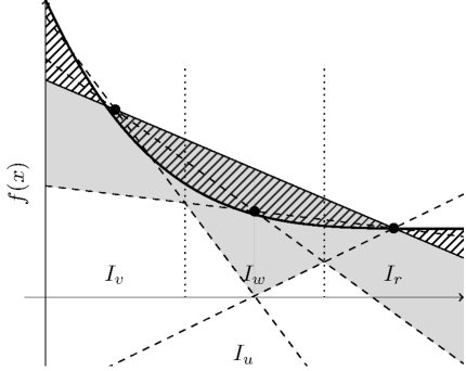 Figure 1
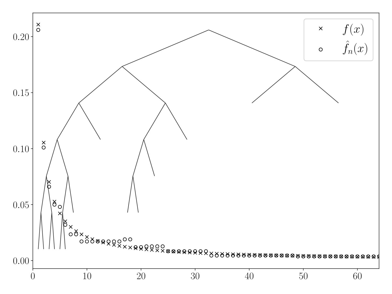 Figure 2
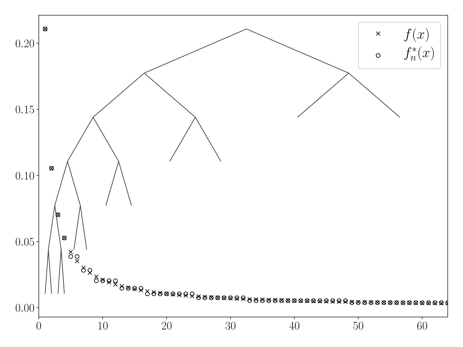 Figure 3
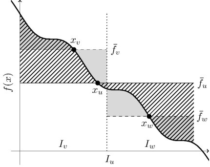 Figure 4
Peer Reviews
No public reviews on file for this paper yet. If you reviewed it on a platform where reviews are public (OpenReview, ICLR, NeurIPS, ICML), you can paste yours below so the community can read it here.
Videos
No videos yet. Explain this paper in a talk, walkthrough, or lecture? Add one.
Discrete minimax estimation with trees
Luc Devroyelabel=e1][email protected] [
Tommy Reddadlabel=e2][email protected] [ McGill University
School of Computer Science
McGill University
3480 University Street
Montréal, Québec, Canada
H3A 2A7
Abstract
We propose a simple recursive data-based partitioning scheme which produces piecewise-constant or piecewise-linear density estimates on intervals, and show how this scheme can determine the optimal minimax rate for some discrete nonparametric classes.
60G07,
density estimation,
minimax theory,
discrete probability distribution,
Vapnik-Chervonenkis dimension,
monotone density,
convex density,
histogram,
keywords:
[class=MSC]
keywords:
\startlocaldefs\endlocaldefs
and
t1Supported by NSERC Grant A3456. t2Supported by NSERC PGS D scholarship 396164433.
Contents
1 Introduction
Density estimation or distribution learning refers to the problem of estimating the unknown probability density function of a common source of independent sample observations. In any interesting case, we know that the unknown source density may come from a known class. In the parametric case, each density in this class can be specified using a bounded number of real parameters, e.g., the class of all Gaussian densities with any mean and any variance. The remaining cases are called nonparametric. Examples of nonparametric classes include bounded monotone densities on , -Lipschitz densities for a given constant , and log-concave densities, to name a few. By minimax estimation, we mean density estimation in the minimax sense, i.e., we are interested in the existence of a density estimate which minimizes its approximation error, even in the worst case.
There is a long line of work in the statistics literature about density estimation, and a growing interest coming from the theoretical computer science and machine learning communities; for a selection of new and old books on this topic, see [13, 14, 16, 22, 32, 33]. The study of nonparametric density estimation began as early as in the 1950’s, when Grenander [20] described and studied properties of the maximum likelihood estimate of an unknown density taken from the class of bounded monotone densities on . Grenander’s estimator and this class received much further treatment over the years, in particular by Prakasa Rao [29], Groeneboom [21], and Birgé [7, 8, 9], who identified the optimal -error minimax rate up to a constant factor, and also gave an efficient adaptive estimator which worked even when the boundedness parameter was unknown. Since then, countless more nonparametric classes have been studied, and many different all-purpose methods have been developed to obtain minimax results about these classes: for the construction of density estimates, see e.g., the maximum likelihood estimate, skeleton estimates, kernel estimates, and wavelet estimates, to name a few; and for minimax rate lower bounds, see e.g., the methods of Assouad, Fano, and Le Cam [13, 14, 16, 35]. See [5, 10, 18, 24] for recent related works in nonparametric shape-constrained regression.
One very popular style of density estimate is the histogram, in which the support of the random data is partitioned into bins, where each bin receives a weight proportional to the number of data points contained within, and such that the estimate is constant with the given weight along each bin. Then, the selection of the bins themselves becomes critical in the construction of a good histogram estimate. Birgé [8] showed how histograms with carefully chosen exponentially increasing bin sizes will have -error within a constant factor of the optimal minimax rate for the class of bounded non-increasing densities on . In general, the right choice of an underlying partition for a histogram estimate is not obvious.
In this work, we devise a recursive data-based approach for determining the partition of the support for a histogram estimate of discrete non-increasing densities. We also use a similar approach to build a piecewise-linear estimator for discrete non-increasing convex densities—see Anevski [1], Jongbloed [26], and Groeneboom, Jongbloed, and Wellner [23] for works concerning the maximum likelihood and minimax estimation of continuous non-increasing convex densities. Both of our estimators are minimax-optimal, i.e., their minimax -error is within a constant factor of the optimal rate. Recursive data-based partitioning schemes have been extremely popular in density estimation since the 1970’s with Gessaman [19], Chen and Zhao [11], Lugosi and Nobel [28], and countless others, with great interest coming from the machine learning and pattern recognition communities [15]. Still, it seems that most of the literature involving recursive data-based partitions are not especially concerned with the rate of convergence of density estimates, but rather other properties such as consistency under different recursive schemes. Moreover, most of the density estimation literature is concerned with the estimation of continuous probability distributions. In discrete density estimation, not all of the constructions or methods used to develop arguments for analogous continuous classes will neatly apply, and in some cases, there are discrete phenomena that call for a different approach. See Jankowski and Wellner [25] for a recent treatment on the properties of a variety of estimators of discrete non-increasing densities.
2 Preliminaries and summary
Let be a given class of probability densities with respect to a base measure on the measurable space , and let . If is a random variable taking values in , we write to mean that
[TABLE]
The notation X_{1},\dots,X_{n}\mathbin{\mathrel{\overset{i.i.d.}{\scalebox{2.0}[1.0]{\sim}}}}f means that for each , and that are mutually independent.
Typically in density estimation, either , is the Borel -algebra, and is the Lebesgue measure, or is countable, , and is the counting measure. The former case is referred to as the continuous setting, and the latter case as the discrete setting, where is more often called a probability mass function in the literature. Throughout this paper, we will only be concerned with the discrete setting, and even so, we still refer to as a class of densities, and as a density itself. Plainly, in this case, signifies that
[TABLE]
Let be unknown. Given the samples X_{1},\dots,X_{n}\mathbin{\mathrel{\overset{i.i.d.}{\scalebox{2.0}[1.0]{\sim}}}}f, our goal is to create a density estimate
[TABLE]
such that the probability measures corresponding to and are close in total variation (TV) distance, where for any probability measures , their TV-distance is defined as
[TABLE]
The TV-distance has several equivalent definitions; importantly, if and are probability measures with corresponding densities and , then
[TABLE]
where for any function , we define the -norm of as
[TABLE]
(In the continuous case, this sum is simply replaced with an integral.) In view of the relation between TV-distance and -norm in (2.2), we will abuse notation and write
[TABLE]
There are various possible measures of dissimilarity between probability distributions which can be considered in density estimation, e.g., the Hellinger distance, Wasserstein distance, -distance, -divergence, Kullback-Leibler divergence, or any number of other divergences; see Sason and Verdú [31] for a survey on many such functions and the relations between them. Here, we focus on the TV-distance due to its several appealing properties, such as being a metric, enjoying the natural probabilistic interpretation of (2.1), and having the coupling characterization (2.3).
If is a density estimate, we define the risk of the estimator with respect to the class as
[TABLE]
where the expectation is over the i.i.d. samples from , and possible randomization of the estimator. From now on we will omit the dependence of on unless it is not obvious. The minimax risk or minimax rate for is the smallest risk over all possible density estimates,
[TABLE]
We can now state our results precisely. Let and let be the class of non-increasing densities on , i.e., set of of all probability vectors for which
[TABLE]
Theorem 2.1**.**
Let be
[TABLE]
There is a universal constant such that, for sufficiently large not depending on ,
[TABLE]
Let be the class of all non-increasing convex densities on , so each satisfies (2.4) and
[TABLE]
Theorem 2.2**.**
Let be
[TABLE]
There is a universal constant such that, for sufficiently large not depending on ,
[TABLE]
We emphasize here that the above results give upper and lower bounds on the minimax rates and which are within universal constant factors of one another, for the entire range of .
Our upper bounds will crucially rely on the next results, which allow us to relate the minimax rate of a class to an old and well-studied combinatorial quantity called the Vapnik-Chervonenkis (VC) dimension [34]: For a family of subsets of , the VC-dimension of , denoted by , is the size of the largest set such that for every , there exists such that . See, e.g., the book of Devroye and Lugosi [16] for examples and applications of the VC-dimension in the study of density estimation.
Theorem 2.3** (Devroye, Lugosi [16]).**
Let be a class of densities supported on , and let be a class of density estimates satisfying for every . Let be the Yatracos class of ,
[TABLE]
For , let be the probability measure corresponding to . Let also be the empirical measure based on X_{1},\dots,X_{n}\mathbin{\mathrel{\overset{i.i.d.}{\scalebox{2.0}[1.0]{\sim}}}}f, where
[TABLE]
Then, there is an estimate for which
[TABLE]
The estimate in Theorem 2.3 is called the minimum distance estimate in [16]—we omit the details of its construction, though we emphasize that if computing takes one unit of computation for any and , then selecting takes time polynomial in the size of , which is often exponential in the quantities of interest; for instance, if is the Yatracos class of , then a simple construction shows that contains all subsets of containing only odd numbers, whence
[TABLE]
where the upper bound is trivial.
Theorem 2.4** (Devroye, Lugosi [16]).**
Let be as in Theorem 2.3, and let . Then, there is a universal constant for which
[TABLE]
Remark 2.5**.**
The quantity in Theorem 2.4 is precisely equal to if is the Borel -algebra on .
Corollary 2.6**.**
Let be as in Theorem 2.3. Then, there is a universal constant for which
[TABLE]
3 Non-increasing densities
This section is devoted to presenting a proof of the upper bound of Theorem 2.1. The lower bound is proved in Appendix A.1 using a careful but standard application of Assouad’s Lemma [2]. Part of our analysis in proving Theorem 2.1 will involve the development of an explicit efficient estimator for a density in .
3.1 A greedy tree-based estimator
Suppose that is a power of two. This assumption can only, at worst, smudge some constant factors in the final minimax rate. Using the samples X_{1},\dots,X_{n}\mathbin{\mathrel{\overset{i.i.d.}{\scalebox{2.0}[1.0]{\sim}}}}f\in\mathcal{F}_{k}, we recursively construct a rooted ordered binary tree which determines a partition of the interval , from which we can build a histogram estimate for . Specifically, let be the root of , where . We say that covers the interval . Then, for every node in covering the interval
[TABLE]
we first check if , and if so we make a leaf in . Otherwise, if
[TABLE]
are the first and second halves of , we verify the condition
[TABLE]
where are the number of samples which fall into the intervals , i.e.,
[TABLE]
The inequality (3.1) is referred to as the greedy splitting rule. If (3.1) is satisfied, then create nodes covering and respectively, and add them to as left and right children of . If not, make a leaf in .
After applying this procedure, one obtains a (random) tree with leaves , and the set forms a partition of the support . Let be the histogram estimate based on this partition, i.e.,
[TABLE]
The density estimate is called the greedy tree-based estimator. See Figure 1 for a typical plot of , and a visualization of the tree .
Remark 3.1**.**
Intuitively, we justify the rule (3.1) as follows: We expect that is at least as large as by monotonicity of the density , and the larger the difference , the finer a partition around and should be to minimize the error of a piecewise constant estimate of . However, even if and were equal in expectation, we expect with positive probability that may deviate from on the order of a standard deviation, i.e., on the order of , and this determines the threshold for splitting.
Remark 3.2**.**
One could argue that any good estimate of a non-increasing density should itself be non-increasing, and the estimate does not have this property. This can be rectified using a method of Birgé [8], who described a transformation of piecewise-constant density estimates which does not increase risk with respect to non-increasing densities. Specifically, suppose that the estimate is not non-increasing. Then, there are consecutive intervals , such that has constant value on and on , and . Let the transformed estimate be constant on , with value
[TABLE]
i.e., the average value of on . Iterate the above transformation until a non-increasing estimate is obtained. It can be proven that this results in a unique estimate , regardless of the order of merged intervals, and that
[TABLE]
3.2 An idealized tree-based estimator
Instead of analyzing the greedy tree-based estimator of the preceding section, we fully analyze an idealized version. Indeed, in (3.1), the quantities are distributed as for , where we define
[TABLE]
If we replace the quantities in (3.1) with their expectations, we obtain the idealized splitting rule
[TABLE]
where we note that , since is non-increasing. Using the same procedure as in the preceding section, replacing the splitting rule with (3.2), we obtain a deterministic tree with leaves , and we set
[TABLE]
i.e., is constant and equal to the average value of on each interval for . We call the idealized tree-based estimate. See Figure 2 for a visualization of and . It may be instructive to compare Figure 2 to Figure 1.
Of course, and both depend intimately upon knowledge of the density ; in practice, we only have access to the samples X_{1},\dots,X_{n}\mathbin{\mathrel{\overset{i.i.d.}{\scalebox{2.0}[1.0]{\sim}}}}f, and the density itself is unknown. In particular, we cannot practically use as an estimate for unknown . Importantly, as we will soon show, we can still use along with Corollary 2.6 to get a minimax rate upper bound for .
Proposition 3.3**.**
[TABLE]
Proof.
Writing out the TV-distance explicitly, we have
[TABLE]
Let , and define . If , then , so assume that . In this case, let and be the left and right halves of the interval , and let and be the average value of on and respectively. Write also
[TABLE]
Refer to Figure 3. We view as the positive area between the curve and the line ; in the figure, this is the patterned area. Then, is the positive area between and on , which is represented as the gray area on in Figure 3, and is the positive area between and on , the gray area on in Figure 3. For , let be the largest point in for which . By the triangle inequality,
[TABLE]
Furthermore,
[TABLE]
where the second equality follows by the choice of . A similar relation holds for , whence
[TABLE]
where this last inequality follows from the splitting rule (3.2), since and . So,
[TABLE]
by the Cauchy-Schwarz inequality. ∎
Proposition 3.4**.**
If and , then
[TABLE]
Proof.
Note that has height at most . Let be the set of nodes at depth in which have at least one leaf as a child, for , and label the children of the nodes in in order of appeareance from right to left in as . Since none of the nodes in are themselves leaves, then by (3.2),
[TABLE]
and in particular since , then so that . In general,
[TABLE]
and this recurrence relation can be solved to obtain that
[TABLE]
Let be the set of leaves at level in . The leaves at level in order from right to left form a subsequence of . Write for the total probability mass of held in the leaves , i.e.,
[TABLE]
By (3.3) and since for each ,
[TABLE]
so that
[TABLE]
Summing over all leaves and using the facts that and ,
[TABLE]
By Hölder’s inequality,
[TABLE]
so finally
[TABLE]
Proof of the upper bound in Theorem 2.1.
The case is trivial, and follows simply because the TV-distance is always upper bounded by .
Suppose next that . In this regime, we can use a histogram estimator for with bins of size for each element of . It is well known that risk of this estimator is on the order of [16].
Finally, suppose that . Let be the class of all piecewise-constant probability densities on which have parts; in particular, . Let be the Yatracos class of ,
[TABLE]
Then, , where is the class of all unions of at most intervals in . It is well known that , so . By Corollary 2.6 and Proposition 3.3, there are universal constants for which
[TABLE]
By Proposition 3.4, we see that for sufficiently large , there is a universal constant such that
[TABLE]
Remark 3.5**.**
Fix and let be the class of all non-increasing densities supported on and bounded from above by . Our method can be applied to prove a minimax rate upper bound . Now, the tree underlying the idealized tree-based estimator is truncated at some given level, say to be specified, and the idealized estimator should take on the average value of the true density on the truncated leaves. Write for the depth of the node in . As in Proposition 3.3,
[TABLE]
The argument of Proposition 3.4 allows us to control the first sum, so that for some universal constant ,
[TABLE]
On the other hand, since for the left child and the right child of , then
[TABLE]
An optimal choice of has that for a universal constant ,
[TABLE]
From here, using the same method as in the proof of Theorem 2.1, it follows that for some universal ,
[TABLE]
4 Non-increasing convex densities
Recall that is the class of non-increasing convex densities supported on . Then, forms a subclass of , which we considered in Section 3. This section is devoted to extending the techniques of Section 3 in order to obtain a minimax rate upper bound on . Again, the lower bound is proved using standard techniques in Appendix A.2.
In this section, we assume that is a power of three. In order to prove the upper bound of Theorem 2.2, we construct a ternary tree just as in Section 3, now with a ternary splitting rule, where if a node has children in order from left to right, we split and recurse if
[TABLE]
Here we obtain a tree with leaves . If has children from left to right, let be the midpoint of for . Let the estimate on be the line passing through the points and . Again, if , then . We refer to as the idealized tree-based estimate for .
Remark 4.1**.**
Since is non-increasing, the operation of Remark 3.2 can again by applied to to obtain a non-increasing estimate for which
[TABLE]
Proposition 4.2**.**
[TABLE]
Before proving this, we first note that by convexity of , the slope of the line passing through and is at least the slope of the line passing through and . Equivalently,
[TABLE]
Proof of Proposition 4.2.
As in the proof of Proposition 3.3, we have
[TABLE]
for . We refer to Figure 4 for a visualization of the quantity , which is depicted as the patterned area.
For , write
[TABLE]
By convexity of ,
[TABLE]
Observe also by convexity that and . So, the line segment between and lies above . Let be the line passing through the points and . Then,
[TABLE]
Let be the midpoint of and , and be the midpoint of and . Let be the leftmost point where intersects , if at all. Then,
[TABLE]
Since the right-hand side is non-negative, then indeed and it must be that lies above to the left of . Similarly, if denotes the rightmost point where the line passing through and intersects , then and lies above to the right of . Therefore,
[TABLE]
It remains to bound and . Let be the point where the line passing through and intersects . As before, this points exists, and since is non-increasing, . Futhermore,
[TABLE]
where the inequality follows from convexity and earlier remarks. A similar argument follows for .
In total,
[TABLE]
The result then follows from the splitting rule (4.1) and the Cauchy-Schwarz inequality. ∎
Proposition 4.3**.**
If and , then
[TABLE]
Proof.
The tree has height at most . Let be the set of nodes at depth in with at least one leaf as a child, for , labelled in order of appearance from right to left in as . By the convex splitting rule (4.1), and since is non-increasing,
[TABLE]
so in particular, , and . In general,
[TABLE]
We claim now that , which we prove by induction; the base case is shown above, and by the induction hypothesis,
[TABLE]
for all , while the cases can be manually verified. Then, by monotonicity of ,
[TABLE]
Let now be the set of leaves at level in . The leaves at level in order from right to left form a subsequence of . Let be the total probability mass of held in the leaves . By (4.3) and since for each ,
[TABLE]
so that
[TABLE]
Summing over all leaves,
[TABLE]
By Hölder’s inequality,
[TABLE]
so finally
[TABLE]
Proof of the upper bound in Theorem 2.2.
The proof is similar to that of Theorem 2.1. ∎
Remark 4.4**.**
As in Remark 3.5, the argument can replicated in the continuous case, for bounded non-increasing convex densities supported on .
5 Discussion
It seems likely, given our results on the idealized tree-based estimators from Section 3.2 and Section 4, that the greedy tree-based estimators also behave well. In particular, we suspect that our greedy tree-based estimators are minimax-optimal within logarithmic factors. We leave this open to future work.
It is also often desirable for nonparametric estimators to be adaptive, in the sense that they attain the optimal minimax rate without depending on some of the important features of the nonparametric class in question. In some cases, an adaptive density estimate can be constructed by first estimating these features, and then building a density estimate assuming the estimated features. For example, in [8], an adapative estimate for non-increasing densities is developed by first estimating the size of the support, and plugging this estimated support size into a non-adaptive estimate. We expect that in this manner, our method can be made adaptive.
The techniques of this paper seem to naturally extend to higher dimensions. Take, for instance, the class of block-decreasing densities, whose minimax rate was identified by Biau and Devroye [6]. This is the class of densities supported on bounded by some constant , such that each density is non-increasing in each coordinate if all other coordinates are held fixed. The discrete version of this class has each density supported on , with the monotonicity constraint. In order to estimate such a density, one could devise an oriented binary splitting rule analogous to (3.2) and carry out a similar analysis as performed in Section 3.2.
Furthermore, we expect that there are many other classes of one-dimensional densities whose optimal minimax rate could be identified using our approach, like the class of -monotone densities on , where a function is called -monotone if it is non-negative and if is non-increasing and convex for all if , and where is non-negative and non-increasing if . This paper tackles the cases of and . Write for the class of -monotone densities on . See Balabdaoui and Wellner [3, 4] for texts concerning the density estimation of -monotone densities. It seems likely that our method could be applied to prove the following conjecture.
Conjecture 5.1**.**
Let be
[TABLE]
Let be fixed. There are constants depending only on such that, for ,
[TABLE]
The main obstacle in proving the above would be the development of good local estimates for -monotone densities, in the same flavor as Proposition 3.3 and Proposition 4.2.
Our approach also likely can be applied to the class of all log-concave discrete distributions, where we recall that is called log-concave if
[TABLE]
See [17, 27, 30] for a small selection of works on the density estimation of -dimensional log-concave continuous densities. The optimal Hellinger distance minimax rate (within logarithmic factors) for this class was recently obtained by Dagan and Kur [12], who showed that it is attained by the maximum-likelihood estimate. There remains a small gap between the best known upper and lower bounds in the TV-distance minimax rate as of the time of writing.
Acknowledgments
We would like to thank the three reviewers and an associate editor for their helpful comments and suggestions.
Appendix A Lower bounds
Lemma A.1** (Assouad’s Lemma [2, 16]).**
Let be a class of densities supported on the set . Let be a partition of , and for and be some collection of functions. For , define the function by
[TABLE]
such that each is a density on . Let agree with on all bits except for the -th bit. Then, suppose that
[TABLE]
and
[TABLE]
Let be the hypercube of densities
[TABLE]
If , then
[TABLE]
A.1 Proof of the lower bound in Theorem 2.1.
Suppose first that . Let be consecutive intervals of even cardinality, starting from the leftmost atom . Split each in two equal parts, and . Let , and set
[TABLE]
It is clear that each is a density. In order for each to be monotone, we require that
[TABLE]
and in particular
[TABLE]
Pick . Since for , it suffices to take
[TABLE]
Let be the smallest even integer at least equal to , so that , and thus
[TABLE]
Since the support of our densities is , then we ask that this last upper bound not exceed . We can guarantee this in particular with a choice of and for which
[TABLE]
Fix . Then,
[TABLE]
so
[TABLE]
On the other hand,
[TABLE]
Now pick
[TABLE]
and for which
[TABLE]
or equivalently,
[TABLE]
Note that now implies that . With this choice, Lemma A.1 implies that
[TABLE]
So we need only verify that these choices of and are compatible with (A.1). Since , then there is an integer choice of in the range
[TABLE]
In particular, we can verify that
[TABLE]
since for all . Moreover, since , then , so that
[TABLE]
where this last inequality holds since for all , so that (A.2) is proved.
When , we argue by inclusion that
[TABLE]
The only remaining case is . In this case, we offer a different construction. Now, each will have size for , where . Fix to be specified later, and set
[TABLE]
We insist that
[TABLE]
for some . Since each must be a density, we need that
[TABLE]
Both of these conditions will be satisfied if we pick
[TABLE]
Furthermore, the largest probability of an atom here is
[TABLE]
for . Then, for , we can compute
[TABLE]
so
[TABLE]
and
[TABLE]
Pick . Then, since and , then , and
[TABLE]
so that
[TABLE]
A.2 Proof of the lower bound in Theorem 2.2.
Let be the partition in Lemma A.1, for an integer to be specified. Let be the smallest element of , and suppose that each is chosen to be a positive multiple of . We will define the functions based on parameters , to be specified. Let linearly interpolate between the points
[TABLE]
on , and between the points
[TABLE]
on . Let linearly interpolate between the points
[TABLE]
on , and between the points
[TABLE]
on . Then, each will be nonincreasing as long as for each , and
[TABLE]
Each will be convex as long as the largest slope on is at most the smallest slope on for each . Equivalently,
[TABLE]
Now, pick for some , to be specified, and
[TABLE]
for which (A.3) is immediately satisfied. The condition (A.4) is then equivalent to
[TABLE]
Pick . It is sufficient to make the choice
[TABLE]
Let be the smallest integer multiple of at least as large as , so that . If , then
[TABLE]
Since the support of our densities is , this upper bound must not exceed , so we impose that
[TABLE]
We must tune in order for each to be a density. By monotonicity, we must have
[TABLE]
and
[TABLE]
so there is a choice of where
[TABLE]
as long as . Now, fix . Then,
[TABLE]
and
[TABLE]
as long as , whence
[TABLE]
Now, pick
[TABLE]
and for which
[TABLE]
or equivalently,
[TABLE]
Note that now implies that . With this choice, Lemma A.1 has
[TABLE]
so it remains to verify that our choices of and are compatible with (A.5). Since , then there is an integer choice of in the range
[TABLE]
In particular, we can verify that
[TABLE]
since for all . Moreover, since , then , so that
[TABLE]
since for all , so that (A.6) is proved.
When , we argue by inclusion that
[TABLE]
It remains to prove the case . Observe that , so the lower bound for follows from Appendix A.1, so we assume that . Now, each will have size for , where . Fix to be specified later, and set
[TABLE]
and
[TABLE]
Each will be non-increasing as long as , and
[TABLE]
for each . Convexity will follow if
[TABLE]
or equivalently,
[TABLE]
We need also that , , and
[TABLE]
Take for to be specified.. Monotonicity follows, and convexity will follow if
[TABLE]
So take each . Then,
[TABLE]
and in particular,
[TABLE]
Take for some , whence
[TABLE]
By monotonicity,
[TABLE]
and
[TABLE]
so that the right choice of satisfies
[TABLE]
Fix . Then,
[TABLE]
and if ,
[TABLE]
Finally, pick . Since and , then , and
[TABLE]
so by Lemma A.1,
[TABLE]
The reference list from the paper itself. Each links out to its DOI / PubMed record.
- 1[1] {barticle} [author] \bauthor \bsnm Anevski, \bfnm Dragi \binits D. ( \byear 2003). \btitle Estimating the derivative of a convex density. \bjournal Statist. Neerlandica \bvolume 57 \bpages 245–257. \bdoi 10.1111/1467-9574.00229 \bmrnumber 2028914 \endbibitem
- 2[2] {barticle} [author] \bauthor \bsnm Assouad, \bfnm Patrice \binits P. ( \byear 1983). \btitle Deux remarques sur l’estimation. \bjournal C. R. Acad. Sci. Paris Sér. I Math. \bvolume 296 \bpages 1021–1024. \bmrnumber 777600 \endbibitem
- 3[3] {barticle} [author] \bauthor \bsnm Balabdaoui, \bfnm Fadoua \binits F. and \bauthor \bsnm Wellner, \bfnm Jon A. \binits J. A. ( \byear 2007). \btitle Estimation of a k 𝑘 k -monotone density: limit distribution theory and the spline connection. \bjournal Ann. Statist. \bvolume 35 \bpages 2536–2564. \bdoi 10.1214/009053607000000262 \bmrnumber 2382657 \endbibitem
- 4[4] {barticle} [author] \bauthor \bsnm Balabdaoui, \bfnm Fadoua \binits F. and \bauthor \bsnm Wellner, \bfnm Jon A. \binits J. A. ( \byear 2010). \btitle Estimation of a k 𝑘 k -monotone density: characterizations, consistency and minimax lower bounds. \bjournal Stat. Neerl. \bvolume 64 \bpages 45–70. \bdoi 10.1111/j.1467-9574.2009.00438.x \bmrnumber 2830965 \endbibitem
- 5[5] {barticle} [author] \bauthor \bsnm Bellec, \bfnm Pierre C. \binits P. C. ( \byear 2018). \btitle Sharp oracle inequalities for least squares estimators in shape restricted regression. \bjournal Ann. Statist. \bvolume 46 \bpages 745–780. \bdoi 10.1214/17-AOS 1566 \bmrnumber 3782383 \endbibitem
- 6[6] {barticle} [author] \bauthor \bsnm Biau, \bfnm Gérard \binits G. and \bauthor \bsnm Devroye, \bfnm Luc \binits L. ( \byear 2003). \btitle On the risk of estimates for block decreasing densities. \bjournal J. Multivariate Anal. \bvolume 86 \bpages 143–165. \bdoi 10.1016/S 0047-259X(02)00028-3 \bmrnumber 1994726 \endbibitem
- 7[7] {barticle} [author] \bauthor \bsnm Birgé, \bfnm Lucien \binits L. ( \byear 1987). \btitle Estimating a density under order restrictions: nonasymptotic minimax risk. \bjournal Ann. Statist. \bvolume 15 \bpages 995–1012. \bdoi 10.1214/aos/1176350488 \bmrnumber 902241 \endbibitem
- 8[8] {barticle} [author] \bauthor \bsnm Birgé, \bfnm Lucien \binits L. ( \byear 1987). \btitle On the risk of histograms for estimating decreasing densities. \bjournal Ann. Statist. \bvolume 15 \bpages 1013–1022. \bdoi 10.1214/aos/1176350489 \bmrnumber 902242 \endbibitem