On topological transitions in metals
Xuzhe Ying, Alex Kamenev

TL;DR
This paper explores whether topological transitions in metals can be detected through transport measurements, finding that certain transport coefficients show clear discontinuities unaffected by bulk metallic transport.
Contribution
It demonstrates that specific transport coefficients exhibit sharp discontinuities at topological transitions, which are not obscured by bulk metallic effects.
Findings
Transport coefficients show discontinuous changes at topological transitions
Discontinuities are robust against bulk metallic transport effects
Certain signatures of topological transitions are detectable in transport measurements
Abstract
We investigate if a sharp topological transition in a metal with a large Fermi surface may be detected in transport measurements. In particular, we address if a skew scattering and a side jump on elastic disorder in the bulk of such a metal masks signatures of the topological transition. We conclude that certain transport coefficients exhibit discontinuous changes across the transition. These discontinuities are not smeared or dwarfed by the bulk metallic transport in a broad range of parameters.
Click any figure to enlarge with its caption.
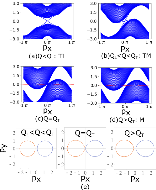 Figure 1
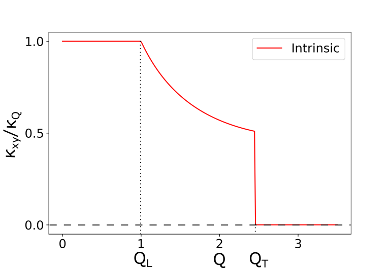 Figure 2
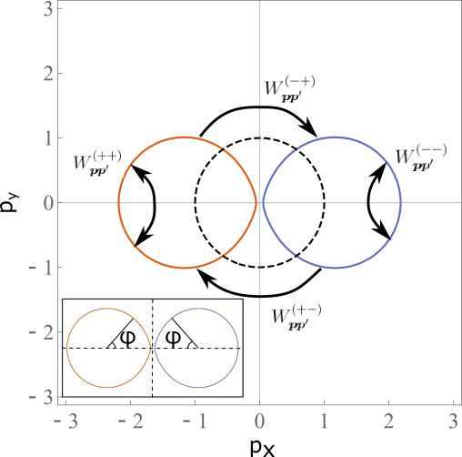 Figure 3
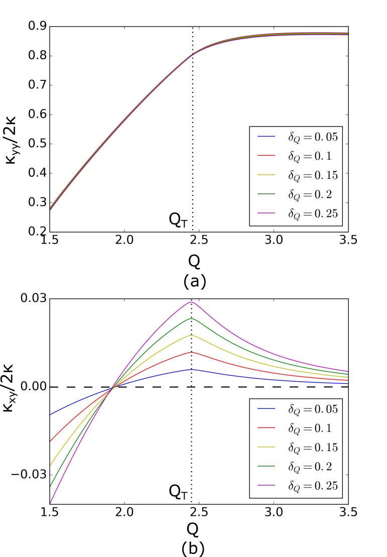 Figure 4
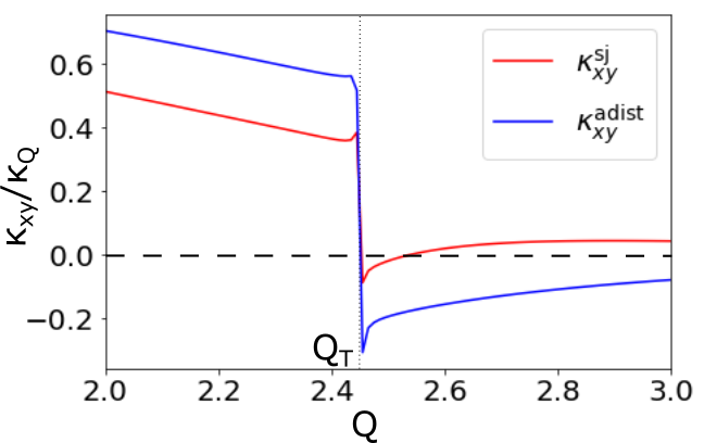 Figure 5
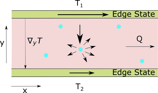 Figure 6
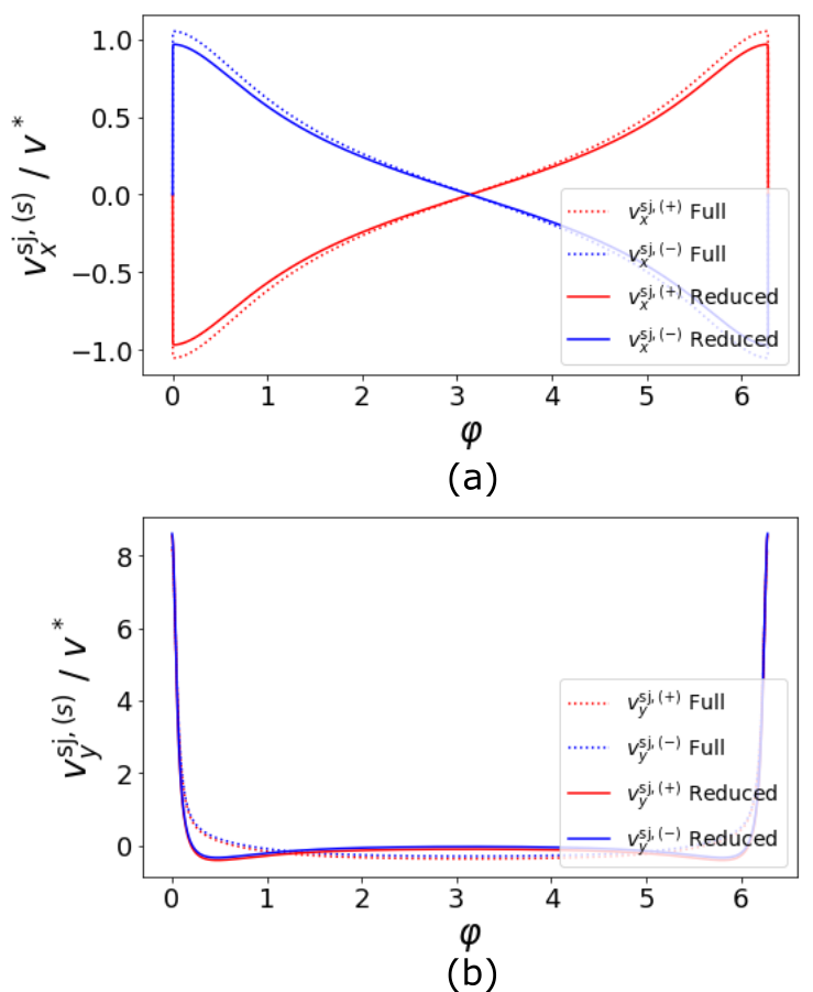 Figure 7
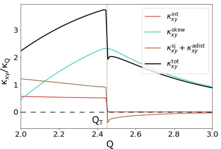 Figure 8
Peer Reviews
No public reviews on file for this paper yet. If you reviewed it on a platform where reviews are public (OpenReview, ICLR, NeurIPS, ICML), you can paste yours below so the community can read it here.
Videos
No videos yet. Explain this paper in a talk, walkthrough, or lecture? Add one.
On topological transitions in metals
Xuzhe Ying
School of Physics and Astronomy, University of Minnesota, Minneapolis, MN 55455, USA
Alex Kamenev
School of Physics and Astronomy, University of Minnesota, Minneapolis, MN 55455, USA
William I. Fine Theoretical Physics Institute, University of Minnesota, Minneapolis, MN 55455, USA
Abstract
We investigate if a sharp topological transition in a metal with a large Fermi surface may be detected in transport measurements. In particular, we address if a skew scattering and a side jump on elastic disorder in the bulk of such a metal masks signatures of the topological transition. We conclude that certain transport coefficients exhibit discontinuous changes across the transition. These discontinuities are not smeared or dwarfed by the bulk metallic transport in a broad range of parameters.
PACS numbers
††preprint: APS/123-QED????????????
I Introduction
Discovery of topological insulators and semimetals Bernevig and Hughes (2013); Shen (2012); Hasan and Kane (2010); Qi and Zhang (2011); Chiu et al. (2016) emphasized a fundamental fact that states of matter may be distinguished by topological indexes. The existence of topological indexes relies on symmetries of the system, rather than a specific Hamiltonian Chiu et al. (2016); Ryu et al. (2010); Wigner (1958); Dyson (1962); Schnyder et al. (2008); Kruthoff et al. (2017). States with different indexes are separated by topological phase transitions, which are often associated with sharp quantized changes of transport coefficients (Hall conductance in the integer quantum Hall effectPrange and Girvin (1987) being the oldest example). Topological transitions are often associated with gapped phases, such as insulators or superconductors. Recent studies of Weyl semimetals Hosur and Qi (2013); Armitage et al. (2018, 2018); Wan et al. (2011); Xu et al. (2015); Lv et al. (2015); Xu et al. (2014); Xu and Zhang (2015) have extended this notion to gapless states, if the chemical potential is tuned to a nodal Weyl (or Dirac) point Baum et al. (2015a, b). For example in Weyl semimetals with mirror symmetry the Hall conductance exhibits a discontinuous quantized change Burkov (2018a, b).
In the present work we investigate if sharp topological transitions may be detected in genuine metals with large Fermi surfaces and a finite density of bulk delocalized states. One may reason that the edge states, if coexist with the bulk extended states, provide a negligible contribution to transport coefficients in the thermodynamic limit. Moreover, if elastic scattering is present it mixes between the edge and the bulk, further degrading any topological signatures. Here we show that these arguments are too simplistic. We conclude that sharp, but non-quantized, discontinuities in transport coefficients persist into the genuine metallic state. Their magnitude is finite and may be comparable with (or even larger than) bulk contributions in the thermodynamic limit. These properties has to be protected by a certain symmetry. We thus refer to them as symmetry protected topological (SPT) metals. If disorder does not break the corresponding symmetry, the transport anomalies are robust to its presence.
To illustrate these points we consider a specific model of SPT metal with the particle-hole symmetry, introduced in Ref. [Ying and Kamenev, 2018]. The model is based on 2D superconductor, which is deformed by an applied flux or a super current. As the super current (hereafter denoted as ) is increased the band structure undergoes two transitions as shown in Fig. 1(a-d). First at , there is a Lifshitz transition from a topological superconductor to the topological metal state. The latter is characterized by two metallic bands with the Fermi surfaces shown in Fig. 1(e). Notice also the two edge states, propagating in the same direction, coexisting with the metallic bands, Fig. 1(b). At , there is the topological transition between the topological and the ordinary metal states. In the clean model the anomalous thermal Hall conductance exhibits a non-quantized discontinuityYing and Kamenev (2018) at .
In the present paper we investigate thermal transport in this model in the presence of a bulk elastic disorder, which preserves the particle-hole symmetry. The schematic setup is indicated in Fig. 2. It assumes an applied thermal gradient, in the -direction. We then evaluate linear response thermal current both in and -directions, which determine longitudinal, , and Hall, , thermal conductances. The latter is, in general, non-zero, because the time-reversal invariance is broken in two ways: (i) the choice of chirality of order parameter and (ii) the applied super current . As illustrated in Fig. 2, acquire contributions from both edge states and bulk elastic scattering.
The main focus of this paper is whether the discontinuity in , found in the clean modelYing and Kamenev (2018), Fig. 3, is observable in the presence of the bulk disorder. We found that this is indeed the case. The skew scattering mechanism results in a continuous contribution to , while the side jump mechanism enhances the discontinuity of the intrinsic contribution. Moreover, in the wide range of parameters the continuous skew scattering contribution is comparable to the discontinuity size. The discontinuity is not smeared by the disorder in the thermodynamic limit. (The discontinuity in should be understood in a scaling limit when and go to zero, while a finite temperature leads to a shop by continuous drop in .)
The structure of the paper is as follows: Section II introduces the model of SPT metal and discusses the intrinsic contribution to the thermal Hall conductance. Section III establishes the appropriate kinetic Boltzmann equation for impurity scattering of quasiparticles occupying particle-like and hole-like conduction bands. SectionIV presents our results and discussion of the topological signatures in the transport coefficients. The rest of the paper provides the necessary details to support the main results: Appendix A-C is devoted to a systematic evaluation of the impurity scattering rates; Appendix D-E is devoted to the side jump displacement and side jump velocities as well as its correction to the thermal Hall conductance.
II Model of SPT metal
We consider a model of SPT metalYing and Kamenev (2018), based on -D superconductor deformed by an applied supercurrent. It is described by the Bogoliubov-de Gennes (BdG) Hamiltonian:
[TABLE]
where
[TABLE]
is electron dispersion close to the bottom of a band and is the chemical potential. The dispersion relation is deformed by the applied flux (or the supercurrent) assumed to be in the -direction and denoted as . Notice that it enters the BdG Hamiltonian as a canonical substitution , where is the Pauli matrix in the particle-hole space.
The off-diagonal part of Eq. (1) is the -wave superconducting gap function. In the continuous limit, adopted here, it is given by
[TABLE]
where is -wave paring amplitude (notice that has a dimensionality of velocity). Throughout the paper we assume that the superconductivity is proximity induced and thus do not try to establish a value of through a self-consistency relation. We also do not discuss a possible suppression of by disorder.
It is instructive to rewrite the Hamiltonian (1) in the matrix notations:
[TABLE]
where is a vector of the Pauli matrices in the particle-hole space. This Hamiltonian has two quasiparticle bands with the energies, Fig. 1:
[TABLE]
where . Hereafter () is the label for the quasiparticle bands and takes the values of . The corresponding quasiparticle wavefunctions (Nambu spinors) are independent on and may be expressed through as
[TABLE]
where \mathcal{N}_{\boldsymbol{p}}=\big{[}2|\boldsymbol{d}(\boldsymbol{p})|(|\boldsymbol{d}(\boldsymbol{p})|+d_{z}(\boldsymbol{p}))\big{]}^{-1/2} is a normalization factor.
The two critical points, see Fig. 1, may be determined from the dispersion relation (5). The two Fermi surfaces form at the Lifshitz transition , when zero energy solution first appear. The topological phase transition takes place at , when the two bands touch at , because .
The Hamiltonian of Eq. (1) possesses the particle-hole symmetry, which is expressed as
[TABLE]
where the particle-hole symmetry operator is defined as , where is complex conjugation operator.
We study thermal Hall conductance of the system described by the Hamiltonian (1) in the geometry indicated in Fig. 2. The thermal gradient is applied in the direction, while the supercurrent flows in the -direction. In the linear response the heat current is given by , where is the thermal Hall conductance. It has two contributions: the intrinsic one due to the edge states and the impurity one due to the skew-scattering.
According to the Kubo-Str̆eda formula Read and Green (2000), the intrinsic (anomalous) thermal Hall conductance (in unit of ) is given by the integrated Berry curvature:
[TABLE]
where the momentum integration runs over the Brillouin zone (BZ) of a proper lattice modelYing and Kamenev (2018). In the superconducting phase the intrinsic conductance is quantized , Fig. 3. In the topological metal phase, , the quantization is broken by the fact that the Fermi surfaces need to be exempt from the BZ summation (at small temperature). At the topological phase transition the intrinsic Hall conductivity discontinuously jumps to zero. The discontinuity in the Hall conductance is a consequence of (and is protected by) the particle-hole symmetry, Eq. (7). These statements have a natural geometric interpretation in terms of the flux of the Berry monopole, as explained in Ref. [Ying and Kamenev, 2018].
We turn now to the contribution to the thermal Hall conductance due to the scattering of bulk quasiparticles on an elastic disorder.
III Kinetic equation treatment of elastic scattering
III.1 Review on Anomalous Hall Effect
Our treatment of the thermal Hall conductance of SPT metals shares some resemblance to the discussion of the anomalous Hall effect (AHE) in ferromagnetic metalsNagaosa et al. (2010); Nagaosa (2006). It was pioneered by Karplus and LuttingerKarplus and Luttinger (1954) who showed that a specific structure of Bloch wave functions gives rise to an anomalous Hall conductivity, which is known as the intrinsic contribution. Soon after, SmitSmit (1955, 1958) pointed out that impurities should play an important role in AHE through anisotropic scattering, which was called a skew scattering. Subsequently systematic diagrammatic calculationsSinitsyn et al. (2007); Goryo (2008); Lutchyn et al. (2009); König and Levchenko (2017); Ado et al. (2015) were developed to include both intrinsic and impurity scattering contribution to the AHE. It was shown that certain diagrams, e.g. ‘Mercedes star’ diagramSinitsyn et al. (2007); Goryo (2008); Lutchyn et al. (2009); König and Levchenko (2017) or ‘X’ and ‘’ diagramsAdo et al. (2015); König and Levchenko (2017), containing higher order terms in Born series must be included to see the effect of skew scattering. At the meantime, it was noticed that the ladder diagrams contributions are on the order of independent of impurity strengthNagaosa et al. (2010). This contribution was named as side jump, indicating that the shift of center of wave packets at impurity scattering events Sinitsyn et al. (2006); Nagaosa et al. (2010).
Alternatively, one can take a kinetic approach based on semiclassical Boltzmann transport equationSinitsyn et al. (2007); Sinitsyn (2008); König et al. (2018), which is equivalent to diagrammatic resummation and typically is more intuitive. In such kinetic approach, the nature of the Bloch waves is taken into account by the so-called anomalous velocity in the semiclassical equation of motion for a Bloch electronSundaram and Niu (1999):
[TABLE]
Here, the Bloch electron is subject to an external force and is the usual group velocity, while is the anomalous velocity. Here is the Berry curvature, given by momentum space curl of Berry connection, . Here, is the periodic part of the Bloch wavefunction.
Impurity scattering may be described by the semiclassical Boltzmann equation with a proper collision integral. It’s important that all orders in Born series for impurity scattering are taken into account by the Lippmann-Schwinger equationSinitsyn et al. (2007); Sinitsyn (2008); Li et al. (2015). In the linear response one can solve the Boltzmann equation to find a stationary distribution function: , where is the equilibrium distribution function and is the deviation from equilibrium due to the external force. Finally the current is given by:
[TABLE]
where in the linear response and . Notice that since the anomalous velocity is already proportional to the external force, the intrinsic contribution relies only on the equilibrium distribution .
In addition, for a Bloch electron, the side jump effects will give additional contributions to the currentSinitsyn et al. (2006):
[TABLE]
This is a result of the center of a wave packet experiencing a displacement upon impurity scattering events. Such a displacement, called the side jump displacement, , depends on the scattering incoming and outgoing states. Here, we briefly reproduce the side jump treatment, following Ref. [Sinitsyn et al., 2006].
One effect of the side jump is that the quasiparticle velocity acquires an additional component. Qualitatively, at each scattering events, the center of a wave packets is shifted by the side jump displacement . Impurity scattering occurs at a rate of the inverse mean free time . As a result, the quasiparticles acquire the side jump velocity , leading to a contribution to the current of the form:
[TABLE]
The second contribution, , originates from the fact that the side jump displacement requires an extra work performed by the external force. As a result, the quasiparticle energy changes by , leading to an ‘anomalous’ correction, , to a stationary distribution function (see below). This contributes to the current as:
[TABLE]
while the total current acquires the form:
[TABLE]
This scheme refers to the electric current, rather than to the thermal one. To access the latter the Wiedemann-Franz law may be employed for noninteracting system as shown by Qin, Niu and ShiQin et al. (2011) based on the Luttinger’s theory of the thermal transportLuttinger (1964). Here we employ a kinetic theory of superconductors recently developed by Li, Andreev and SpivakLi et al. (2015). These authors were interested in a transport of thermally excited quasiparticles in the gapped regime. We adopt their approach to the low-temperature transport in the deformed model with the two Fermi surfaces.
III.2 Kinetic Equation
Here we develop a semiclassical Boltzmann equation approach for the quasiparticles with the energies and wavefunctions given by Eqs. (5) and (6) correspondingly. The applicability of this approach is limited to a weak disorder, where the longitudinal conductance is much larger than the conductance quantum. At low temperature this is only possible at . In this regime the two Fermi surfaces are present and a weak disorder induces elastic scattering between states close to the Fermi surfaces as shown in Fig. 4.
Within each band, labeled as , the quasiparticle states are assigned a distribution function, . As in Fig. 4, the elastic scattering induces intra as well as inter band transitions, which enter the Boltzmann equation through the collision integrals (see eg. Ref. [Kamenev, 2011]). The coupled Boltzmann equations for the two bands take the form:
[TABLE]
where is quasiparticle velocity. Notice that the anomalous velocity due to Berry curvatureSundaram and Niu (1999) is not included here since it gives rise to the intrinsic contribution of Hall conductivity and does not mix with impurity contribution in the limit of linear response.
As indicated in Fig. 4, the collision integrals involve several scattering processes between quasiparticle states: scattering within each band with scattering rates and ; scattering between two bands with scattering rates and . Thus the elastic collision integrals take the form:
[TABLE]
where the integral is defined as . Here, in the collision integral, the two distribution functions are evaluated at a slightly different location. The difference in position is given by the side jump displacement:
[TABLE]
We now assume that a small temperature gradient is applied in -direction and look for the deviations of the distribution functions from their equilibrium form:
[TABLE]
where is the equilibrium Fermi distribution. The deviations from equilibrium Fermi distribution can be separated into two part: (i) is the solution of the Boltzmann equation with elastic collision by neglecting the side jump effect; (ii) is called the ‘anomalous distribution function’, compensating the effect of the position change (side jump) over the impurity scattering events. These two parts can be solved independently, due to the linearity of the collision integral, Eq. (16) (and the Boltzmann equation, Eq. (15)). Since we restricted ourselves to the linear response, we only seek for the deviations and proportional to the temperature gradient.
III.3 Skew Scattering
Neglecting for now the side jump effect, the collision integral, Eq. (16), reads:
[TABLE]
The effect of skew scattering manifested itself in the asymmetry of the scattering rate. Namely, in the absence of the time-reversal symmetry the matrix elements are not symmetric:
[TABLE]
Or more explicitly (as will be derived in Appendix A-C), the scattering rates have the following formLi et al. (2015):
[TABLE]
where the azimuthal angle () defines the direction of the momentum (). And is a small deflection angle, which depends on the metallic density of states and the impurity potential (see Eq. (53) in Appendix A):
[TABLE]
Its presence is crucial for the asymmetrical property Eq. (20), given that the prefactors are symmetric.
Therefore the collision integral does not conform to the detailed balance. As a result, it can’t be written in the form . Nevertheless the form (19), linear in the distribution functions, is the correct one and it is this form that follows from the Keldysh formalismSturman (1984); Kamenev (2011)111We are indebted to Anton Andreev for discussions of this issue. The collision integral still vanishes at equilibrium, , where is the Fermi function. This is enforced by the unitarity conditionLifshitz and Pitaevskij (1981):
[TABLE]
As a result, only the deviation from equilibrium distribution frunction is present in Eq. (19).
The collision integral, Eq. (19), is set equal to the kinetic terms on the left hand side of Boltzmann equation, Eq. (15). With a small temperature gradient in -direction, the linear response approximation reads:
[TABLE]
If the scattering rates are known, this equation may be solved for the linear deviations . The thermal conductivity is found then from calculating the heat current:
[TABLE]
where and are the thermal Hall and longitudinal thermal conductivity respectively.
III.4 Side Jump
The side jump refers to the shift of the center of a Bloch wavepacket upon an impurity scattering eventSinitsyn et al. (2006): , where a quasiparticle is scattered from state to . This leads to the two effects: (i) the quasiparticles acquire an additional velocity and as a result, there is an additional current denoted as ; (ii) the distribution function acquires an anomalous part and the corresponding correction to the current is denoted as . While treating the side jump, we disregard the small skewness of the scattering rates, i.e. we assume here . In other words we consider the scattering rates to be detailed balance related: . The error we commit by this approximation is of the higher order in and .
The jump velocity is given by:
[TABLE]
while the corresponding contribution to the transversal current is given by:
[TABLE]
The anomalous distribution originates from the collision integral, Eq. (16). Notice that the latter is nonlocal in space. It can be transformed into a local form by expanding the distribution function in terms of the side jump displacement:
[TABLE]
The anomalous distribution serves to compensating the nonlocality, by fulfilling the condition:
[TABLE]
This can be further simplified employing the linear response relation:
[TABLE]
Equation (29) can be thus cast into the form:
[TABLE]
where the collision integral is given below with a symmetric scattering rate:
[TABLE]
Solving this equation for the ‘anomalous distribution’ , one obtains the second contribution to the transversal current:
[TABLE]
An important observation is that the side jump contribution to the thermal Hall conductance is independent of mean free time . This can be seen by noticing that the side jump current , while the side jump velocity is proportional to the scattering rate: . Moreover, as we show below, the side jump contribution to the thermal Hall conductance is of the same order as the intrinsic part.
IV Results and discussion
With the general framework formulated above we solved the Boltzmann equation in the linear response approximation and evaluated the corresponding thermal conductivites. Details of these calculations are delegated to the Appendices. Here we present the results.
Figure 5 summaries our results for the skew scattering contribution to the diagonal and off-diagonal thermal conductivity. They are measured in units of (twice) the thermal conductivity of the normal metal ():
[TABLE]
Here is the diffusion constant (with and being the normal metal Fermi velocity and relaxation time respectively), is dimensionless 2D normal state conductance and is thermal conductance quanta. The topological phase transition takes place at . We present the results for only, since in the opposite limit the system is a thermal insulator and the quasiparticle contribution is exponentially small.
One notices that the diagonal conductivity is essentially independent on the asymmetry factor and approaches the normal metal value above the topological transition. The off-diagonal exhibits approximately linear dependence on , which in turn is linear in the weak disorder amplitude, , Eq. (22). This is due to the fact that the off-diagonal part, originating from the skew scattering, is proportional to the antisymmetric part of the rate matrix, Eq. (56). The off-diagonal conductivity exhibits maximum at the topological phase transition and slowly approaches zero deep into the non-topological metallic phase, . Notice that: (i) is a continuous function of through the topological transition and (ii) its magnitude is much less than that of the diagonal . The latter observation follows from the fact that
[TABLE]
where is the symmetric part of the scattering rates and we employ Eq.(55). In the limit , assumed hereafter, it follows that .
The latter fact is important for the possibility to detect the topological transition within the metallic phase. Indeed, the kinetic theory developed here is valid in the weak scattering limit, when normal-state dimensionless conductance is large . Consequently the diagonal thermal conductivity . However the off-diagonal one appears to be of the order . This value may be comparable to (or even smaller than) the thermal conductance quantum , even in a good metal, . The skew scattering contribution to the diagonal conductivity, , on the other hand, is much larger than all other terms. We thus do not discuss other contributions to the diagonal conductivity.
Figure 6 shows the side jump contributions to the off-diagonal thermal conductivity . It exhibits a discontinuity at the topological phase transition. The magnitude of the discontinuity is given by (see Appendix D-E):
[TABLE]
Those are of the same sign and order of magnitude as the discontinuity in the intrinsic part . In addition, they should be added together. Therefore, the total discontinuity at the topological phase transition is:
[TABLE]
The discontinuity is non-quantized and depends on band-structure parameters, such as in our model. On the other hand, it does not depend on impurities concentration and strength, as long as the sample dimensions exceed elastic mean free path. In the opposite limit of a ballistic sample, the discontinuity is smaller and is given solely by the intrinsic contribution. Comparing the discontinuity with the smooth skew scattering part (35), we observe that the two may be comparable in a wide range of the relevant dimensionless parameters, such as the ratio , the normal state conductance and asymmetry factor .
Figure 7 summarises the total off-diagonal conductivity, along with its three constitutive components: the skew-scattering contribution, Eq. (35), the intrinsic contribution Eq. (8) and side jump, Eq. (36). The total exhibits discontinuous jump at the topological phase transition in the limit of small temperature. This discontinuity takes place in the presence of the metallic bulk states and bulk disorder, as long as the particle-hole symmetry, Eq. (7), is preserved. Therefore the topological transition exhibits the sharp signature in transport measurements not only in gapped phases, but also in gapless systems with finite density of states at the Fermi level. Unlike the gapped case, the corresponding jump is non-quantized.
One may be concerned if impurity scattering between the bulk and the edge states may change these conclusions. Such processes are not accounted for in the developed kinetic approach. Indeed, the intrinsic part knows only about the equilibrium distribution function, Eq. (8), not affected by the impurity scattering. Formally this is due to the fact that the anomalous velocity is already proportional to and thus to the linear response accuracy one should take the unperturbed distribution function. Physically, it reflects the fact that the edges are in local equilibrium with the adjacent bulk heat reservoir. Since the edge states are exponentially confined to the sample’s boundaries, Fig. 2, they can’t be affected by the perturbation , which is spread across the bulk. As a result, the impurity scattering between an edge and an adjacent bulk is exactly the same as in equilibrium: it does not affect the occupation of the edge state and does not change the corresponding thermal current. This reasoning breaks down very close to the topological transition, where the edge states spread into the bulk and thus acquire sensitivity to the perturbation . This happens in earnest only for , where is the localization length critical exponent. This leads to a finite size smearing of the discontinuity, which is not present in the thermodynamic limit . The discontinuity is smeared at a finite temperature, much like the integer quantum Hall transitions.
V Acknowledgments
We are grateful to A. Andreev, M. Ye, D. Chichinadze, A. Levchenko and M. Sammon for useful discussions. We are also grateful to a referee for his/her insistence to include consideration of the side jump effect. This work was supported by NSF Grant No. DMR-1608238.
Appendix A Scattering rates
We turn now to the microscopic evaluation of the scattering rates . The off-diagonal response, , is a consequence of the asymmetry in the scattering rate, Eq. (20), which appears in the absence of the time-reversal symmetry and is known as the skew scattering mechanism. In our model the time reversal symmetry is already broken by superconductivity, Eq. (3), and the supercurrent further introduces anisotropy to the system. As a result, the detailed balance is violated, which leads to anomalous transport in SPT metal.
We restrict ourselves with the weak point-like impurities with impurity density . Therefore the scattering rates are given by:
[TABLE]
where is the scattering amplitudes of an individual impurity between quasiparticle states.
Scattering process should contain all orders in Born series and the Lippmann-Schwinger equation is used to find scattering -matrix , which determines scattering amplitudesLi et al. (2015); Sturman (1984); Sinitsyn (2008). Consider a generic Hamiltonian:
[TABLE]
where is the Hamiltonian free of impurities and is the impurity potential. The scattering -matrix is formally defined by the Lippmann-Schwinger equationAltland and Simons (2010):
[TABLE]
where is the bare Green’s function. The scattering amplitudes between quasiparticle states could be determined from -matrix:
[TABLE]
where is the quasiparticle eigenstate.
Following Li, Andreev and SpivakLi et al. (2015) we first solve Eq. (40) in the original particle-hole basis and then transform to the quasiparticle basis as:
[TABLE]
A remark about notations is due: the labels are labeling particle-hole states, while are labeling the quasiparticle bands. Thus, the summation indices is over particle-hole states and are the elements of the quasiparticle wavefunctions, given by Eq. (6). In the particle-hole basis equation (40) takes the formLi et al. (2015):
[TABLE]
where and . In this same basis the Hamiltonian takes the form of the BdG Hamiltonian (4) and the point-like impurity potential is independent of momenta . Therefore, the scattering matrix is independent of momenta and is only a function of the frequency . Hence Eq.(43) can be rewritten in a compact way as a matrix equation in the particle-hole spaceLi et al. (2015):
[TABLE]
where the Green function is defined as . The formal solution for the scattering matrix is:
[TABLE]
Close to the topological phase transition, , the summation of the Green function over momenta may be separated into two parts: and , as indicated in Fig. 4. The Hamiltonian, Eq.(4), has very different asymptotic behavior in these two regimes. Since we considered small temperatures, only the quasiparticle states near the zero energy are important. Therefore, the quantity of interest here is actually . For small momenta, , the Hamiltonian in Eq.(4) is approximately a tilted massive Dirac Hamiltonian with the mass of :
[TABLE]
with corrections on the order of and . Hence, summation of the Green function over momenta is:
[TABLE]
It’s clear that the terms with numerator linear in momenta and vanish upon summation. Hence the result is proportional to the mass term . Performing the integration, as detailed in Appendix B, one finds:
[TABLE]
For large momenta , one can neglect the off-diagonal terms in the Hamiltonian (3), leaving two copies of the normal metal decoupled from each other.
Therefore, summation of the Green results in the 2D density of states of a metal:
[TABLE]
where is a density of states at the chemical potential. Taken together Eqs. (48) and (49) yield:
[TABLE]
The scattering matrix can be obtained from Eq. (45)Li et al. (2015):
[TABLE]
where
[TABLE]
It’s clear that the scattering matrix is a smooth function of the supercurrent around the topological phase transition at . As explained below, the phase is responsible for the skew scattering. Close to the topological phase transition one finds from Eq. (52):
[TABLE]
approximately a constant proportional to the impurity potential .
To find scattering amplitudes between the quasiparticle states one needs to transform the particle-hole matrix (51) to the quasiparticle basis according to Eq. (42):
[TABLE]
where the quasiparticle spinors are given by Eq. (6). The scattering rates are defined as , where is impurity density. A straightforward calculation outlined in Appendix C leads to the following structure of the rate matrix:
[TABLE]
where and are symmetric with respect to the momenta interchange and and are the azimuthal angles of the corresponding momenta (i.e. ). As can be seen from Eq. (68), the dependence of the rates on the azimuthal angles comes solely from superconductivity present in the Hamiltonian (1). This in turn leads to an antisymmetric part of the rate matrix
[TABLE]
which is responsible for the off-diagonal thermal conductivity.
Once the scattering rates are found (see Appendix C), the linearized Boltzmann equation (24) may be solved numerically for the deviation of the distribution function from its equilibrium value. It is convenient to parametrize such deviations in terms of angles labeling position along the two, , Fermi surfaces, see inset in Fig. 4,
[TABLE]
where is a suitably chosen cutoff (typically a few dozens). The absence of the term reflects the elastic nature of the scattering, which ensures quasiparticle number conservation at any energy. We solve for the harmonic amplitudes and and then evaluate linear response current according to Eq. (25).
One can do the same for solving for the ‘anomalous distribution’ , once the side jump velocity is found in the Appendix D-E.
Appendix B Calculations leading to Eq.(48)
In this section, we show details for deriving Eq.(48):
[TABLE]
The first step is to replace summation by integration:
[TABLE]
Notice the Green’s function takes the following form at small momenta:
[TABLE]
The terms in the numerator here linear in momenta vanishes upon integration. Thus, the quantity to calculate is:
[TABLE]
The angular integration results in:
[TABLE]
where is the step function. Its presence puts an additional constraint on the integration over the magnitude of momentum . To simplify further calculations we focus on the vicinity of the topological phase transition and thus , while . The above integral thus simplifies down to:
[TABLE]
Noticing that the ‘mass’ , where , one arrives at Eq.(48).
Appendix C Scattering Rates
Here we derive explicit expressions for the scattering rates in terms of functions in the BdG Hamiltonian Eq. (4). As discussed in the main text one needs to transform the scattering -matrix , Eq. (51), in the particle-hole basis to the quasiparticle basis with the help of the wavefunctions through Eq.(38):
[TABLE]
where according to Eq.(54):
[TABLE]
where the spinors may be written in terms of and the azimuthal angle as:
[TABLE]
This particular form of wavefunctions is a direct result of -wave superconductivity and leads to a nontrivial angular dependence of . The scattering matrix in particle-hole space is:
[TABLE]
This way one finds for the scattering amplitudes between the quasiparticle states:
[TABLE]
The scattering rates are then found with the help of Eq.(38):
[TABLE]
Although cumbersome, these expressions allow to estimate the magnitude of thermal Hall conductivity, , resulting in Eq.(35). Indeed, the typical symmetric and antisymmetric parts of have the form:
[TABLE]
Assuming and , one finds:
[TABLE]
Appendix D Side Jump Displacement and Velocity
D.1 Side Jump Displacement and Velocity
In this section, we turn to the microscopic calculation of the side jump displacement and the side jump velocity . The actual calculation is rather tedious. Instead of providing all the details, we simply sketch the derivation process. Then we present the most relevant terms in the side jump velocity and estimate the discontinuity in the off-diagonal conductance around topological phase transition.
We employed the gauge invariant definition of the side jump displacement derived in Ref. [Sinitsyn et al., 2006]:
[TABLE]
where the differential operator is defined as . The terms in the first line is also known as the Berry connection, . Given the quasiparticle wavefunctions Eq. (6), it’s straightforward to show:
[TABLE]
As before, is the quasiparticle band index.
The second line involves the scattering amplitude , which is derived in the previous Appendix C. Here, we make further simplifications. First, as argued in Sec. III, we took when the side jump is under consideration. This is the same as neglecting the interplay between the skew scattering and the side jump effect. Second, we focus ourselves to the regime very close to the topological phase transition, . With those two simplifications, the scattering amplitudes take a simple form following Eq. (54):
[TABLE]
The impurity potential does not depend on the momenta. As a result:
[TABLE]
Or equivalently:
[TABLE]
where is the unnormalized wavefunction. The unnormalized wavefunction simplifies the detailed calculations a little bit. Taking the derivative on the argument of a complex valued function (in this case or ) gives:
[TABLE]
In the numerator, means taking the imaginary part of the quantity in the square bracket.
Above we derived the working expressions for the side jump displacement. However, it’s more important to define the side jump velocity:
[TABLE]
Close to the topological phase transition , the scattering rates is given by:
[TABLE]
Following this procedure, one would end up with a rather cumbersome expression. Fortunately, if one focus on the vicinity of topological phase transition, the side jump velocity is governed by part of the full expression:
[TABLE]
Fig. 8 is a comparison of the side jump velocity obtained from the full definition, Eq. (78), and the reduced expression, Eq. (80).
Before explaining the features of Eq. (80), we should remind our readers that the terms in Eq. (80) are not the only nonvanishing terms for the side jump velocity. However, those are the only terms that change sign over the topological phase transition. Therefore, they should give rise to a discontinuity in the off-diagonal conductance, . From now on, we simply focus on Eq. (80).
In Eq. (80), both expressions change sign over the topological phase transition. In Eq. (80a), the side jump velocity in -direction is explicitly proportional to a factor of , where is the Dirac mass in Eq. (46).
Meanwhile, for the side jump velocity in -direction Eq. (80b), the factor of changes sign. The normalization factor is \mathcal{N}_{\boldsymbol{p}}=\big{[}2|\boldsymbol{d}(\boldsymbol{p})|(|\boldsymbol{d}(\boldsymbol{p})|+d_{z}(\boldsymbol{p}))\big{]}^{-1/2}. For small momentum , the quasiparticles are described by Eq. (46). The side jump velocity takes the following form:
[TABLE]
As a result, the side jump velocity in both - and -directions is at least proportional to the sign of . Thus, they should change sign over the topological phase transition. This directly leads to the discontinuity in the thermal Hall conductance, .
The second observation is that both expressions are proportional to the inverse of the mean free path . is the mean free time. As discussed, the direct result of this feature is that the side jump contribution to is independent of the impurity strength, if we confine ourselves to the diffusive regime.
D.2 Estimation of the Discontinuity in
With the side jump velocity in Eq. (80), we were able to estimate the discontinuity in the thermal Hall conductance with relaxation time approximation. The correct sign and order of magnitude could be found. Technical details are provided in the Appendix E.
Start with the discontinuity in :
[TABLE]
With relaxation time approximation, Eq. (24) reduces to:
[TABLE]
It’s straightforward that the distribution function is:
[TABLE]
The first part of the side jump current could be defined from Eq. (27):
[TABLE]
Notice the presence of mean free time in the above equation. It will cancel the dependence in the side jump velocity. Thus, the side jump contribution should be independent of mean free time (or mean free path ). By performing the integration explicitly as in Appendix E, one finds:
[TABLE]
The discontinuity in can be read off directly to the second order in :
[TABLE]
In the second line, was factored out.
Similarly, the anomalous distribution function can be estimated with the relaxation time approximation:
[TABLE]
The associated current is given by Eq. (33):
[TABLE]
Following the similar procedure, the discontinuity in was estimated to be:
[TABLE]
Appendix E Integration over side jump velocity
In this appendix, we provide the details for evaluation of the integrals of side jump contribution to the off-diagonal thermal conductance.
Start with :
[TABLE]
With relaxation time approximation, Eq. (24) reduces to:
[TABLE]
It’s straightforward that the distribution function is:
[TABLE]
The first part of the side jump current could be defined from Eq. (27):
[TABLE]
The trick to perform the integration is to change the integration measure:
[TABLE]
Notice that both the side jump velocity and the group velocity () are proportional to . Therefore the integrand in the current expression is even in . One could just focus on the upper plane with . Focusing on the upper half plane would introduce a factor of in the last expression in Eq. (95). Then the current expression reduces to
[TABLE]
Further simplification can be made if one think about really low temperature. Namely, only a tiny energy window around Fermi surfaces is under consideration:
[TABLE]
The second integral gives a factor of:
[TABLE]
The first integral should be understood as an integration on the Fermi surfaces. Namely, the momenta are implicitly constrained by . The integral could be evaluated analytically:
[TABLE]
Details of this integral is as follows:
[TABLE]
First, notice that the momenta are constrained by , or more explicitly:
[TABLE]
As a result, we could change the integration variable to:
[TABLE]
Meanwhile, could also be expressed in terms of :
[TABLE]
Notice that . With all those quantities, the integral transforms to:
[TABLE]
In the last line, . The integration in the last line could be evaluated analytically:
[TABLE]
Therefore, putting everything together, we obtained:
[TABLE]
where the summation over the band index gives an additional factor of . The discontinuity in can be read off directly to the second order in :
[TABLE]
In the second line, was factored out.
Similarly, the anomalous distribution function can be estimated from Eq. (31) with the relaxation time approximation:
[TABLE]
The associated current is given by Eq. (33):
[TABLE]
Following the similar procedure, we arrived at the expression:
[TABLE]
As before,
[TABLE]
The other integral can be calculates as follows:
[TABLE]
Keep in mind that the momenta are constrained by the condition . We focus on small momentum regime, where the side jump velocity takes a large value:
[TABLE]
where is the cutoff when the quasiparticles ceased to behave like a Dirac particle. The above integration could be evaluated in two steps. First:
[TABLE]
Notice that the ‘exact’ expression for . For small momentum , we could simplify . At the same time, has approximately the same limitation. With this simplification, the integration is straightforward:
[TABLE]
Second, we evaluate:
[TABLE]
For momentum in the region , one direct simplification is that . Namely, is neglected. With this simplification, the constraint reads:
[TABLE]
The integration reduces to
[TABLE]
Putting together the two-step integration, we get:
[TABLE]
With the results for the integrations, one finds the current to be:
[TABLE]
The discontinuity in was estimated to be:
[TABLE]
The reference list from the paper itself. Each links out to its DOI / PubMed record.
- 1Bernevig and Hughes (2013) B. A. Bernevig and T. L. Hughes, Topological Insulators and Topological Superconductors (Princeton University Press, Princeton, NJ, 2013).
- 2Shen (2012) S.-Q. Shen, Topological Insulators (Springer-Verlag, Berlin, 2012).
- 3Hasan and Kane (2010) M. Z. Hasan and C. L. Kane, Rev. Mod. Phys. 82 , 3045 (2010) . · doi ↗
- 4Qi and Zhang (2011) X.-L. Qi and S.-C. Zhang, Rev. Mod. Phys. 83 , 1057 (2011) . · doi ↗
- 5Chiu et al. (2016) C.-K. Chiu, J. C. Y. Teo, A. P. Schnyder, and S. Ryu, Rev. Mod. Phys. 88 , 035005 (2016) . · doi ↗
- 6Ryu et al. (2010) S. Ryu, A. P. Schnyder, A. Furusaki, and A. W. W. Ludwig, New J. Phys. 12 , 065010 (2010).
- 7Wigner (1958) E. P. Wigner, Ann. Math. 67 , 325 (1958).
- 8Dyson (1962) F. J. Dyson, J. Math. Phys. 3 , 1199 (1962).