Optimal Control of Hybrid Optomechanical Systems for Generating Non-Classical States of Mechanical Motion
Ville Bergholm, Witlef Wieczorek, Thomas Schulte-Herbrueggen and, Michael Keyl

TL;DR
This paper demonstrates how coupling a two-level system to a cavity optomechanical system and applying optimal control techniques can generate non-classical states of mechanical motion with negative Wigner function regions.
Contribution
It introduces a hybrid optomechanical system with a two-level system and develops optimal control methods to produce non-classical mechanical states beyond linear regimes.
Findings
Successfully drives the system to non-classical target states
Uses realistic experimental parameters for optimization
Naive control schemes are ineffective for non-classical state preparation
Abstract
Cavity optomechanical systems are one of the leading experimental platforms for controlling mechanical motion in the quantum regime. We exemplify that the control over cavity optomechanical systems greatly increases by coupling the cavity also to a two-level system, thereby creating a hybrid optomechanical system. If the two-level system can be driven largely independently of the cavity, we show that the non-linearity thus introduced enables us to steer the extended system to non-classical target states of the mechanical oscillator with Wigner functions exhibiting significant negative regions. We illustrate how to use optimal control techniques beyond the linear regime to drive the hybrid system from the near ground state into a Fock target state of the mechanical oscillator. We base our numerical optimization on realistic experimental parameters for exemplifying how optimal control…
Click any figure to enlarge with its caption.
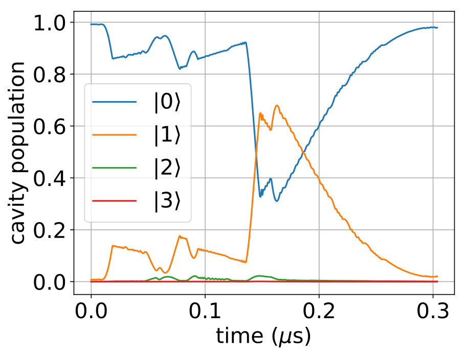 Figure 1
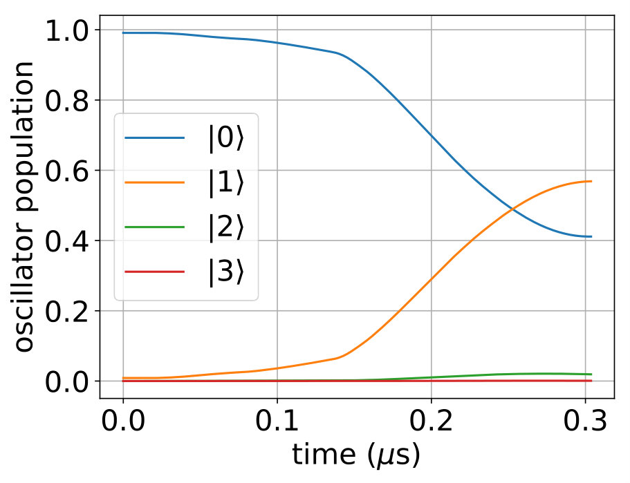 Figure 2
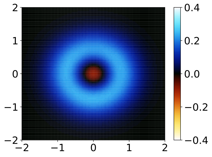 Figure 3
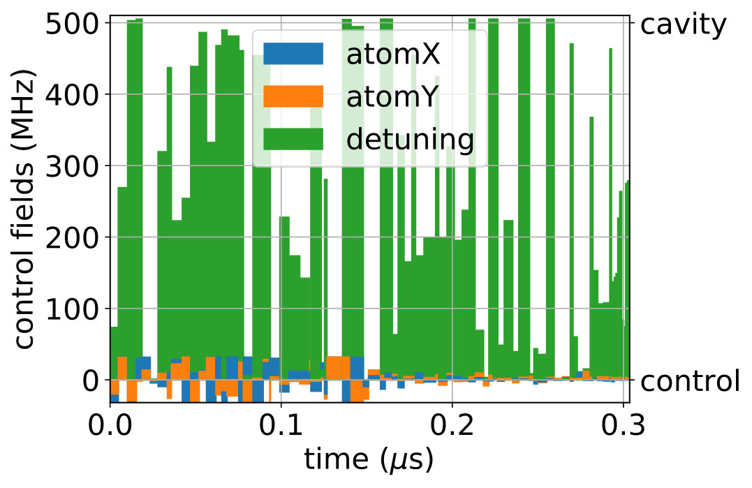 Figure 4
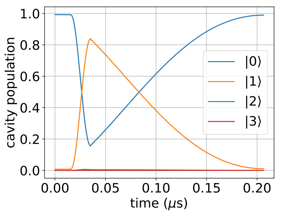 Figure 5
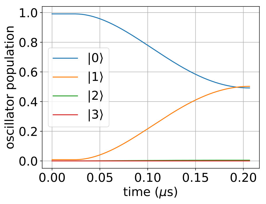 Figure 6
 Figure 7
 Figure 8
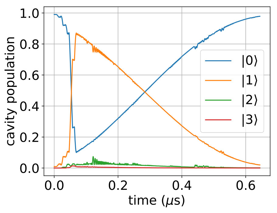 Figure 9
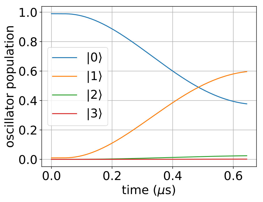 Figure 10
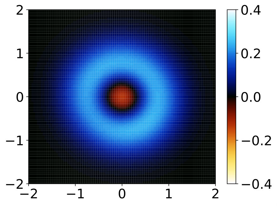 Figure 11
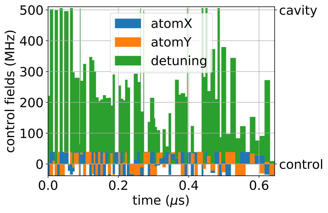 Figure 12
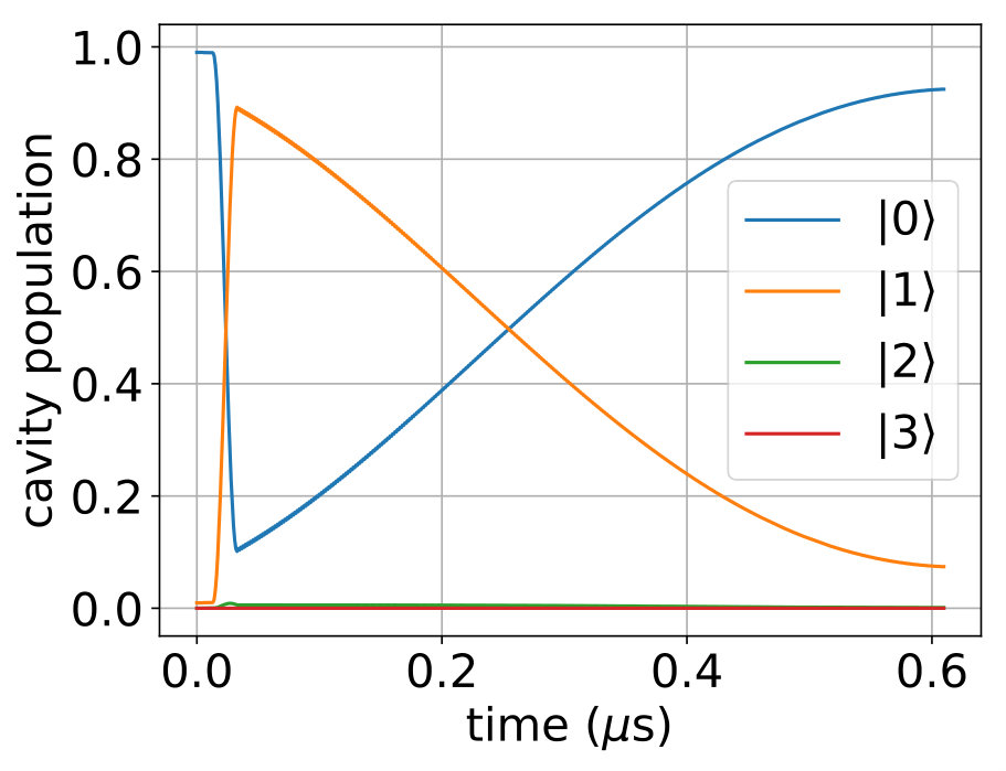 Figure 13
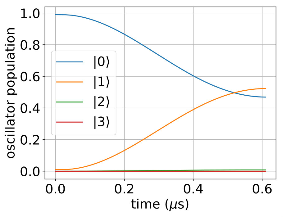 Figure 14
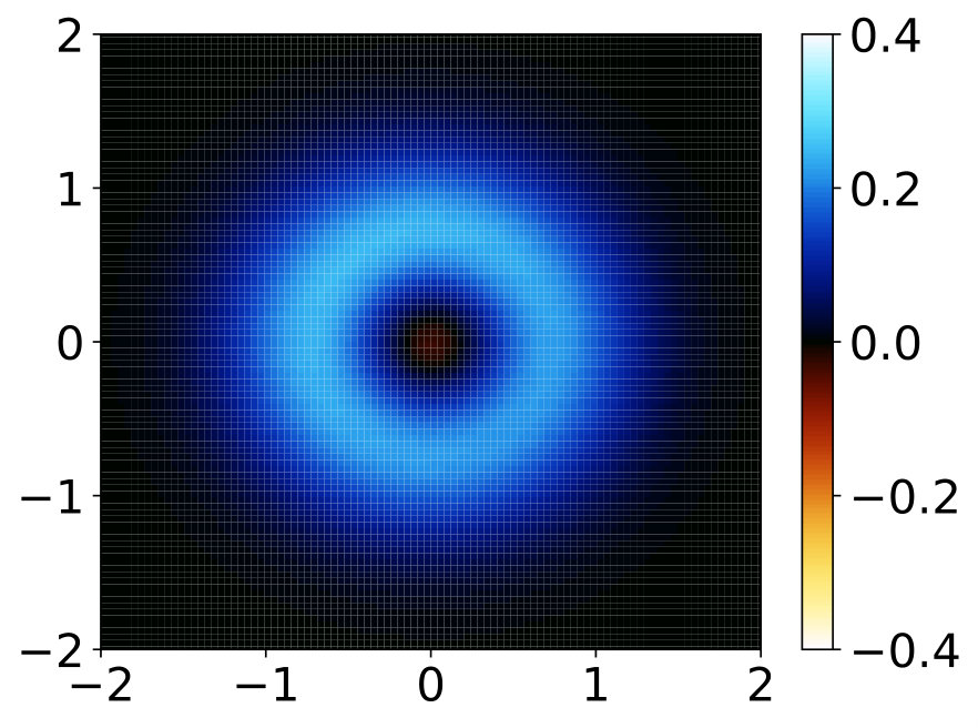 Figure 15
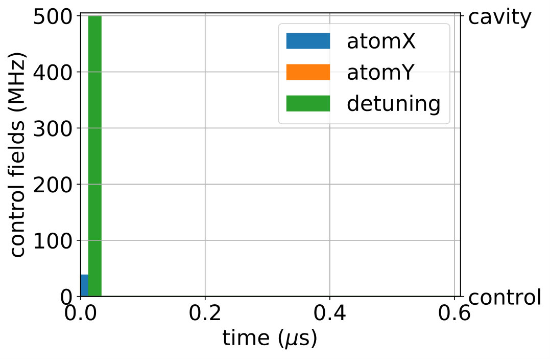 Figure 16
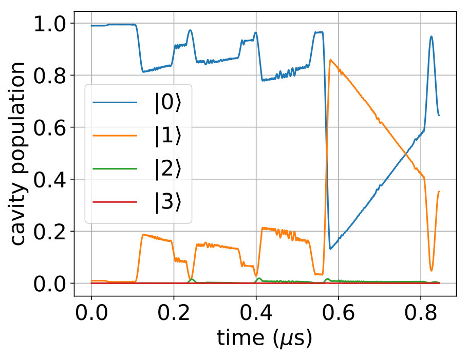 Figure 17
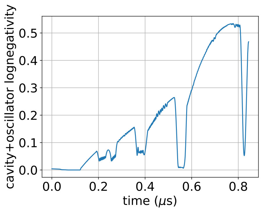 Figure 18
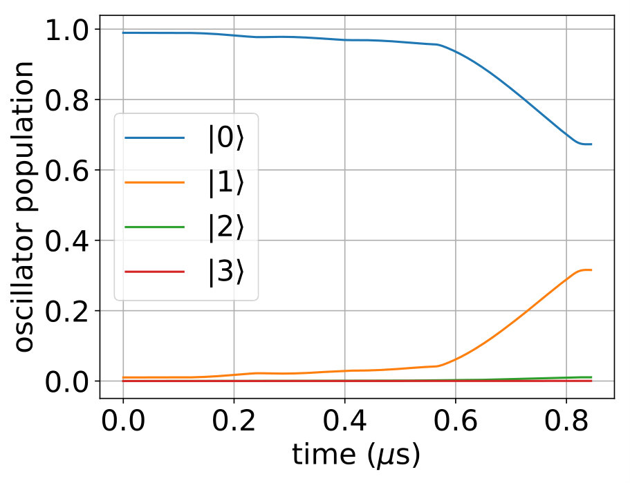 Figure 19
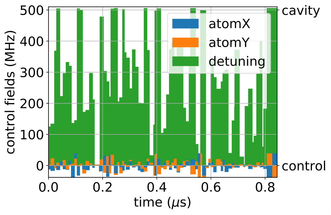 Figure 20
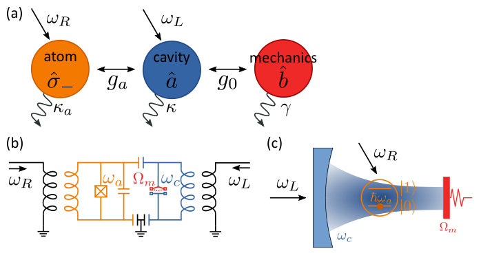 Figure 21
| parameter set | sequence type | dim | fidelity | log-negativity | figure |
|---|---|---|---|---|---|
| Set 2 | optimal control | 3 | 0.6451 | 0.4643 | |
| 4 | 0.6450 | 0.4680 | 6 |
| symbol | meaning | Set 1 | Set 2 | ||
|---|---|---|---|---|---|
| transformed atom annihilation operator | |||||
| transformed cavity annihilation operator | |||||
| transformed oscillator annihilation operator | |||||
| cavity shift (boosts the linearized coupling) | 100 | 120 | |||
| oscillator shift, real part | |||||
| oscillator shift, imaginary part | |||||
| atom resonance frequency | 9–13.5 | GHz | |||
| cavity resonance frequency | 10.188 | GHz | |||
| oscillator resonance frequency | 15.9 | MHz | |||
| atom-cavity coupling | 12.5 | MHz | |||
| cavity-oscillator coupling | kHz | ||||
| boosted atom-cavity coupling | GHz | ||||
| boosted cavity-oscillator coupling | MHz | ||||
| atom decay rate | 1 | MHz | |||
| cavity decay rate | MHz | ||||
| oscillator decay rate | 150 | Hz | |||
| cavity-driving laser frequency | |||||
| cavity-driving laser amplitude | 3.18 | 3.82 | GHz | ||
| cavity-driving laser phase | |||||
| atom control frequency | |||||
| atom control amplitude | 32 | 38 | MHz | ||
| atom control phase | |||||
| cavity resonance frequency shift | MHz | ||||
| shifted cavity resonance frequency | 10.188 | GHz | |||
| laser detuning | |||||
| shifted laser detuning | |||||
| shifted atom detuning | |||||
| shifted atomic control detuning | |||||
| temperature | mK | ||||
| atom Boltzmann factor | |||||
| cavity Boltzmann factor | |||||
| oscillator Boltzmann factor | |||||
| expected number of oscillator phonons | |||||
| effective oscillator decay rate | kHz | ||||
| measure | definition | Set 1 | Set 2 |
|---|---|---|---|
| sideband resolution | 15.9 | 79.5 | |
| cavity-oscillator cooperativity | 298 | 343 | |
| cavity-oscillator coupling-dissipation ratio | 1.2 | 1.8 | |
| atom-cavity cooperativity | 156 | 781 | |
| atom-cavity coupling-dissipation ratio | 12.5 | 12.5 |
| term | significance | Set 1 | Set 2 |
|---|---|---|---|
| driving laser, co-rotating | 99 | 120 | |
| driving laser, counter-rotating | 0.078 | 0.094 | |
| atomic control, counter-rotating | 0.00082 | 0.00098 | |
| , non-linear part | 0.00075 | 0.00019 | |
| , two-mode squeezing | 0.038 | 0.011 | |
| , counter-rotating | 0.00063 | 0.00063 | |
| , counter-rotating | 0.063 | 0.076 |
Peer Reviews
No public reviews on file for this paper yet. If you reviewed it on a platform where reviews are public (OpenReview, ICLR, NeurIPS, ICML), you can paste yours below so the community can read it here.
Videos
No videos yet. Explain this paper in a talk, walkthrough, or lecture? Add one.
Optimal Control of Hybrid Optomechanical Systems for Generating Non-Classical States of Mechanical Motion
Ville Bergholm
Dept. Chemistry, Technical University of Munich (TUM), 85747 Garching, Germany and
Munich Centre for Quantum Science and Technology (MCQST), Schellingstr. 4, 80799 München, Germany
Witlef Wieczorek
Department of Microtechnology and Nanoscience (MC2), Chalmers University of Technology, 41296 Göteborg, Sweden
Thomas Schulte-Herbrüggen
Dept. Chemistry, Technical University of Munich (TUM), 85747 Garching, Germany and
Munich Centre for Quantum Science and Technology (MCQST), Schellingstr. 4, 80799 München, Germany
Michael Keyl
Dahlem Centre for Complex Quantum Systems, Free University of Berlin, 14195 Berlin, Germany
(March 17, 2024)
Abstract
Cavity optomechanical systems are one of the leading experimental platforms for controlling mechanical motion in the quantum regime. We exemplify that the control over cavity optomechanical systems greatly increases by coupling the cavity also to a two-level system, thereby creating a hybrid optomechanical system. If the two-level system can be driven largely independently of the cavity, we show that the non-linearity thus introduced enables us to steer the extended system to non-classical target states of the mechanical oscillator with Wigner functions exhibiting significant negative regions. We illustrate how to use optimal control techniques beyond the linear regime to drive the hybrid system from the near ground state into a Fock target state of the mechanical oscillator. We base our numerical optimization on realistic experimental parameters for exemplifying how optimal control enables the preparation of decidedly non-classical target states, where naive control schemes fail. Our results thus pave the way for applying the toolbox of optimal control in hybrid optomechanical systems for generating non-classical mechanical states.
I Introduction
In view of quantum technologies (see, e.g., Dowling and Milburn (2003)), optimal control techniques provide an increasingly useful toolbox to take quantum hardware to the limits of reaching target states with high fidelity, precision, sensitivity and robustness—one prominent example being feedback stabilization of predefined photon-number states in a box Sayrin et al. (2011); Haroche (2013). Systematic strategies to unlock and exploit the hardware potential in experimental settings with the help of optimal control methods can be found in a quantum control roadmap Glaser et al. (2015).
A recent physical system that has been added to the family of quantum hardware are mechanical resonators Schwab and Roukes (2005); Poot and van der Zant (2012); Aspelmeyer et al. (2014). Pioneering experiments realized cooling of mechanical motion to the quantum ground state by direct cryogenic O’Connell et al. (2010) or by laser-based cooling techniques Chan et al. (2011); Teufel et al. (2011a). A current focus lies on generating non-classical mechanical states, which are required to fully leverage mechanical resonators for applications in quantum metrology Geraci et al. (2010); Johnsson et al. (2016), as quantum transducers Stannigel et al. (2010); Safavi-Naeini and Painter (2011) or for fundamental tests of quantum mechanics Marshall et al. (2003); Romero-Isart (2011); Schmöle et al. (2016). Along these lines, the control over excitations of single phonons has been demonstrated by coupling mechanical motion to artificial atoms O’Connell et al. (2010); Chu et al. (2017) or to cavity light fields Riedinger et al. (2016); Hong et al. (2017).
Cavity optomechanical systems constitute a successful platform for quantum control of mechanical motion Aspelmeyer et al. (2014). Importantly, the optomechanical interaction is intrinsically non-linear and, thus, would lend itself for directly generating non-classical states of mechanical motion Bose et al. (1997); Mancini et al. (1997); Marshall et al. (2003). However, in real-world physical realizations Chan et al. (2011); Teufel et al. (2011b), the single-photon strong coupling regime Rabl (2011); Nunnenkamp et al. (2011) required for exploiting this non-linearity has not been achieved to date, with notable exceptions in cold atom optomechanics setups Murch et al. (2008); Brennecke et al. (2008). Therefore, it is common practice to boost the optomechanical interaction by a coherent drive at the cost of losing its intrinsic non-linear character. Non-classical mechanical states can nevertheless be generated when coupling an optomechanical system to other non-linear systems Hammerer et al. (2009); O’Connell et al. (2010); Pflanzer et al. (2013); Ramos et al. (2013), by introducing the non-linearity in the measurement process Jacobs et al. (2009); Vanner et al. (2013a); Riedinger et al. (2016); Clarke and Vanner (2019), by injecting non-classical states of light Akram et al. (2010); Rabl (2011); Nunnenkamp et al. (2011); Riedinger et al. (2016); Hong et al. (2017), or by coupling to the squared mechanical position quadrature Thompson et al. (2008); Sankey et al. (2010); Vanner (2011); Romero-Isart et al. (2011).
In the present work we focus on a hybrid optomechanical system for non-classical state generation. More precisely, we choose a system consisting of a mechanical resonator that is parametrically and weakly coupled to a cavity, which in turn is strongly coupled to a two-level system (see Fig. 1). Such a system has been analyzed before in the context of strong atom-mechanics coupling Hammerer et al. (2009), dissipative state engineering Pflanzer et al. (2013), tripartite polaron dynamics Restrepo et al. (2014), and optical bistability Jiang et al. (2016). It finds direct relevance in present experimental implementations Lecocq et al. (2015a); Schmidt et al. (2018) and potential future implementations in nano-optic Tiecke et al. (2014); Chan et al. (2011) or ion-trap scenarios Neumeier et al. (2018).
In our study, we first establish controllability of the optomechanical hybrid system in the absence of dissipation processes. We then apply optimal control algorithms and suggest concrete controls in an experimentally realistic setting for generating a non-classical state of mechanical motion. As an example, we choose to focus on generating a single-phonon Fock state and use numerical optimization to find pulse sequences for optimally generating such a state. In order to be close to realistic experimental settings, we adapt parameters from the electromechanics implementation of Ref. Lecocq et al. (2015a) for illustrating the gain of optimal control over established control techniques.
In many instances, quantum optimal control Butkovskiy and Samoilenko (1990); Peirce et al. (1988); Krotov (1996); Khaneja et al. (2005); D’Alessandro (2007) provides both framework and algorithms to go beyond conventional approaches. In cavity optomechanics, standard control techniques imply making use of interactions in the linearized regime using cw-driving Vitali et al. (2007); Paternostro et al. (2007); Wilson-Rae et al. (2007); Marquardt et al. (2007); Hofer et al. (2011); Hofer and Hammerer (2015, 2017), multi-tone driving Kronwald et al. (2013); Brunelli et al. (2018); Houhou et al. (2018) or pulsed driving Vanner et al. (2011); Vanner (2011); Vanner et al. (2013a) for generating entangled states Palomaki et al. (2013); Riedinger et al. (2018); Ockeloen-Korppi et al. (2018), squeezed states Wollman et al. (2015); Pirkkalainen et al. (2015); Lecocq et al. (2015b) or for performing state tomography Vanner et al. (2013b). The leap that optimal control techniques offer is to accommodate the specifics of the system for finding experimental protocols that can be run in a much shorter time frame or that achieve a higher fidelity in state preparation. Optimal control may, thus, find control sequences that embrace limitations in the system’s parameters, which otherwise may prevent generating desired target states. Indeed, optimal control schemes have already been analyzed for optomechanical systems for enhancing cooling performance Wang et al. (2011); Machnes et al. (2012); Triana et al. (2016), for generating optomechanical entanglement Stefanatos (2017), or for squeezing Basilewitsch et al. (2019). A recent account on treating optomechanical systems including feedback as linear control systems can be found in Hofer and Hammerer (2017).
In the present work, we move to the framework of bilinear control systems Elliott (2009) and cutting-edge algorithms Machnes et al. (2011) to show how (by adding a two-level atom) this setting allows for generating a non-classical mechanical Fock state in a parameter regime, where conventional steering methods fail. Our methodology can be extended for optimal generation of mechanical Schrödinger cat states Mancini et al. (1997); Brunelli et al. (2018) or cubic phase states Houhou et al. (2018), provided the truncation of the Hilbert space required for our computational optimization can be extended to higher Fock state numbers.
Our paper is structured as follows: in Sec. II we present the Hamiltonian of the hybrid optomechanical system and derive a drift and control part, in Sec. III we discuss the controllability of our system from a general perspective, in Sec. IV we present the numerical algorithms our optimal control optimization is based on, in Sec. V we use optimal control based on realistic experimental parameters to generate a single phonon Fock state and finally, in Sec. VI, we discuss the results and give an outlook on future work. Appendix A summarizes a detailed derivation of the Hamiltonian of the hybrid optomechanical system treated here and lists the entire parameter setting.
II Theoretical models: drift and control Hamiltonian
The optomechanical system of interest is described in the lab frame by the Hamiltonian
[TABLE]
where and are the annihilation operators of the cavity and the oscillator, and the last term represents driving of the optical cavity by a laser. The quadrature of the cavity is defined as the direction of the driving. The driving Rabi frequency is connected to the laser power and the cavity decay rate by .
The system may be made more amenable to control by adding a strongly non-linear element in the form of a controllable two-level atom in the cavity with the Hamiltonian
[TABLE]
Above, the three terms represent the atom itself, the atom-cavity coupling, and a classical control signal driving the atom, respectively. denote the atomic raising and lowering operators.
Dissipation processes to be taken into account are decay processes in the cavity and damping of the mechanical oscillator. The former are described by the Lindblad operator . This assumes that the effective temperature of the cavity surroundings is zero, which is a good approximation for most cavities. To describe the damping in the mechanical oscillator we use the Lindblad operators and , where is the effective decay rate, the base decay rate, the expected number of oscillator phonons in the steady state, and the oscillator Boltzmann factor. Finally, we describe the atomic decay by with the atom decay rate . Combining all dissipation processes we end up with a standard Markovian master equation
[TABLE]
where is the density operator of the overall system.
To get a set of equations better prone for numerical simulation we simplify the described setup in a number of steps (cf. Appendix A for detailed calculations):
We transform the cavity into a frame co-rotating with the laser by applying the unitary . This is followed by a rotating wave approximation (RWA) to drop the counter-rotating terms. 2. 2.
Simultaneously, we transform the atom by and apply again the RWA. 3. 3.
Due to driving the cavity with a laser field, the cavity (without atom, and oscillator) ends up in a coherent steady state . From a computational point of view it is useful to consider oscillations around (and not around the cavity vacuum), since this step allows more radical truncations of the physical Hilbert space. Hence we apply a phase space shift to get new creation and annihilation operators , with
[TABLE]
with appropriately chosen parameters ; cf. Appendix A.3 for exact values. The shift, in particular, will act as a multiplicative factor to in a new linear interaction term coupling the cavity and the oscillator. 4. 4.
The atomic operators are replaced by the phase-rotated versions with
[TABLE] 5. 5.
If the average photon number is high, the non-linear optomechanical interaction term can be linearized and replaced by a hopping interaction. 6. 6.
At the end we drop another counter-rotating interaction term (i.e. another RWA), to make the system completely time independent (apart from the control terms).
Finally, we end up with the following drift and control Hamiltonians:
[TABLE]
and with the modified Lindblad operators
[TABLE]
Now we can replace the Hamiltonian part of Eq. (3) by and the by the of Eq. (6) to get a new master equation
[TABLE]
Its time dependence is entirely wrapped up in the control functions with . In principle one could also control the frequency and amplitude of the laser drive (see, e.g., Machnes et al. (2012)) thus leading to a modulation of the cavity-laser detuning and the cavity-oscillator coupling . For simplicity, in this work we keep the cavity laser drive constant in order to exploit the drive continuously for three tasks: (i) cooling of the oscillator into its ground state, (ii) using the swap interaction between cavity and oscillator and (iii) separating the interaction time scales between the atom-cavity and the cavity-oscillator couplings. Yet, other parameter regimes or target states may require control of the external laser drive, which we leave for future work.
In our case, the optimal control task now amounts to finding control amplitudes such that an appropriately chosen initial state evolves after a time into some best approximation to a given target state of the mechanical oscillator (after tracing out cavity and atom). An obvious candidate for the initial state is the steady state the system evolves into if we only consider laser driving of the cavity. The steady state is influenced by the presence of the atom and thus changes with the detuning of the atom. If the detuning is large, is close to the ground state. Numerical calculations can be found in Appendix A.4.
III Controllability
Before analysing an experimentally realistic scenario, let us sketch that asking for controllability of the hybrid optomechanical system proposed is well-posed from a control theoretical point of view. To this end, we neglect dissipation for the moment and solely look at the coherent evolution given by .
It is well known that the extent of control over harmonic oscillator modes or light modes greatly increases by coupling the modes to a controllable two-level atom, whereby the system actually becomes fully controllable Law and Eberly (1996); Brockett et al. (2003); Rangan et al. (2004). For the Jaynes-Cummings model of one or several atoms coupled to an oscillator mode, some of us showed in Keyl et al. (2014) that breaking the symmetry by controls on the atom leads to approximate full controllability (in the strong operator topology). Here acts on the atom and is the number operator of the oscillator.
Systematically extending similar lines, approximate controllability of the Jaynes-Cummings-Hubbard model (now comprising an entire network of cavities each containing one mode and one two-level atom, where the interaction between two cavities is given by a hopping term) is analyzed in detail in Heinze and Keyl (2018). It is shown that any pure state of the overall system can be prepared with arbitrarily small error starting from an arbitrary pure initial state by controlling the atoms individually and the cavity-cavity interactions globally. Yet when looking at the mechanical oscillator as another cavity, this result does not directly cover our case, because the oscillator in turn is not coupled to another controllable two-level system. Moreover, the reasoning in Heinze and Keyl (2018) indicates that the given scenario is a minimal requirement for full controllability. Hence, in our case this means one could not prepare any pure state of the overall system either.
Fortunately, the overall state of the system is not needed, since in the extended system suggested here, we are interested in the partial state of the oscillator only, where the situation is much easier. Consider the atom-cavity subsystem first. This part is well studied and known to be fully controllable Brockett et al. (2003); Rangan et al. (2004); Yuan and Lloyd (2007); Bloch et al. (2010); Keyl et al. (2014) in the sense that one can reach with arbitrary small error any pure state of atom and cavity from any initial state by using and only—with not needed except for speed-up.
In contrast, cavity and oscillator alone just follow quasi-free dynamics, which is much more limited. Even when allowing for control of the coupling strength, one is far from full controllability, since the time-evolution operator would be confined to the Schrödinger representation of the metaplectic group Folland (2016). However, with the Hamiltonian components given in Eqs. (4) and (5), it is easy to see that—in entire analogy to the classical phase space—the states of cavity and oscillator become (approximately) flipped after a certain time. Hence a possible strategy to control the overall system is: prepare a state of the cavity first and wait until it flips over to the oscillator. This indicates that one can actually prepare any pure state of the oscillator from an arbitrary pure initial state.
In this idealized controllability assessment of our setup, note that atom-cavity coupling is 10 times stronger than the boosted cavity-oscillator coupling thus leading to a separation of time scales. In simple cases this allows to treat atom-cavity and cavity-oscillator system independently as described above. In other words, a simple cavity state can be prepared before the swapping to the oscillator has effectively started. After this preparation phase, the effects of the still present atom-cavity interaction can be continuously compensated by further control pulses on the atom (such that the swapping can go on undisturbed). This approximation only breaks down if the preparation of the cavity state takes so long that it gets compromised by the cavity-oscillator swap. In that case it may be necessary to resort to controlling the parameter in order to manipulate the cavity-oscillator coupling . Another limitation to the controllability assessment just outlined is dissipation. So both the numerical analysis and the experiment have to address mixed states with the dissipation time limiting the overall control time.
The state-of-the-art of using optimal control with linear feedback for optomechanical systems has been summarized in the recent comprehensive review by Hofer and Hammerer Hofer and Hammerer (2017). Note that the systems thus far addressed do not use the interaction with an atom, but rather a feedback loop from homodyne detection on a beam coupled out of the cavity. The information gathered is then used to drive the cavity with a linear feedback Hamiltonian of the form
[TABLE]
where are annihilation and creation operators of the cavity and is the amplitude of the feedback signal. From the point of view of Lie-algebraic systems and control theory, such systems come with limitations: since all terms in the overall Hamiltonian are at most quadratic in creation and annihilation operators, Hamiltonians of that form constitute a finite dimensional Lie algebra. Therefore, the manifold of time evolution operators thus generated is also finite dimensional (no matter whether the terms are time dependent or not) and can thus be described by finitely many parameters. A given initial state with Wigner function evolves following a classical phase flow, i.e. the solution of the initial value problem for the classical system. The latter, however, is but a multi-dimensional harmonic oscillator driven by a force which is constant in space. Hence, if has no negative parts, this cannot change under such a form of time evolution. For instance, if is Gaussian, it stays Gaussian all the time.
Adding an atom interacting with the cavity as used in our context is meant to overcome exactly these limitations. One may look at it as adding a third oscillator which only interacts via its two lowest levels with the rest of the system. The corresponding interaction term cannot be written as a quadratic polynomial in creation and annihilation operators of the now three-dimensional oscillator system. Therefore it breaks the covariance of the canonical commutation relations given in terms of the metaplectic representation, and the reasoning from the previous paragraph does not apply. Therefore, adding a two-level atom allows for preparing any state of the harmonic oscillator subsystem from any initial state.—The remaining question of how severe the restrictions imposed by a realistic dissipative system are, and up to which degree the theoretical possibilities can actually be exploited by pulse sequences shall be explored in the sequel by some examples using numerical optimal control.
IV Numerical algorithms
In view of going beyond Gaussian states, the extended hybrid optomechanical setting lends itself to be treated as a bilinear control system Elliott (2009) with states following
[TABLE]
Its form is determined by a non-switchable drift term , while the control is brought about by (typically piecewise constant) control amplitudes governing the time dependence of the otherwise constant control operators . The connection to the Lindblad master Eq. (II) above is given by the identifications111 Here, , and are linear ‘superoperators’ acting on the state . For numerics, a convenient concrete representation takes as the column vector stacking all columns of the matrix . With the conventions of Ref. (Horn and Johnson, 1991, Chp. 4), Hamiltonian commutator superoperator components are obtained as , and the Lindbladian dissipator as \hat{\Gamma}:=\sum_{k}\bar{V}_{k}\otimes V_{k}-\tfrac{1}{2}\big{(}{\rm 1\negthickspace l}{}\otimes(V_{k}^{\dagger}V_{k})+(V_{k}^{\top}\bar{V}_{k})\otimes{\rm 1\negthickspace l}{}\big{)}. The Lindblad master eqn. (II) can then readily be read and treated as vector differential equation of the type .
[TABLE]
Given this equation of motion, the optimal control task then amounts to minimizing the Euclidean distance between the (possibly mixed) target state on the one hand and the final state of the system on the other hand. Typically results after steps of time propagation in slots of piecewise constant quantum maps (with for as uniform width of time intervals) propagating the state according to Eqn. (II)
[TABLE]
Likewise, the distance between the truncations to the sublevels of interest and may be taken, or alternatively, a Lagrange-type penalty term may be added to the cost functionals discussed in the outlook.
Explicitly allowing for changing purity and mixed target states requires some generalization of the standard task (with constant purity) discussed in Ref. Machnes et al. (2011). To this end, we extract from the (squared) Euclidean distance (in terms of the Frobenius norm )
[TABLE]
those terms depending on time (and therefore on the controls) and rescale to arrive at the cost functional
[TABLE]
Taking the derivative with respect to the control amplitude in the time slot then gives
[TABLE]
where the difference instead of just now takes care of the purity change. In the unital case, the derivative of the propagating quantum map would make use of being normal (so in slight abuse of language it has orthogonal eigenvectors associated to the real eigenvalues ) to take the form described in Aizu (1963); Wilcox (1967) and used in Machnes et al. (2011):
[TABLE]
In the general (non-normal) case mostly encountered here we have to resort to finite differences according to
[TABLE]
where has to be sufficiently small in the sense . Given , steepest-descent of the cost functional with the controls would follow a recursion in reading
[TABLE]
with as step size, while the standard Newton update would take the form
[TABLE]
with denoting the inverse Hessian in the iteration. For convenience the array of piecewise constant control amplitudes is concatenated to the control vector for each time slot , while is the corresponding gradient vector. In this work we use the bfgs quasi-Newton algorithm Nocedal and Wright (2006) to approximate the inverse Hessian as explained in Machnes et al. (2011).
V Results by optimal control
The numerical optimization results presented in this section are for two variants of the circuit cavity electromechanical system described in Lecocq et al. (2015a). It consists of a mechanical oscillator coupled to a microwave cavity. The cavity mode is further coupled to a superconducting qubit (“atom”). In the original implementation the atom-cavity coupling is fairly strong, MHz, but the cavity-oscillator coupling is much weaker, Hz. In all of our simulations we have artificially boosted the single-photon optomechanical coupling strength by one order of magnitude, which together with the boost resulting from coherent driving of the cavity brings the optomechanical system in the required strong-coupling regime222 Note that one could in principle boost instead of to reach the required strong coupling regime between the mechanical oscillator and the cavity. However, boosting also increases the interaction of the atom with the cavity, which complicates the control scheme as discussed in Appendix A.5..
The two parameter sets we use are
- •
Set 1: Coupling enhancement factor , is boosted by a factor of to kHz, cavity decay rate MHz and the device is operated at a temperature of mK.
- •
Set 2: Coupling enhancement factor , is boosted by a factor of to kHz, cavity decay rate MHz and the device is operated at a temperature of mK. Compared to Set 1, we have assumed an optical cavity with a smaller linewidth, which allowed us to reduce the boost of the optomechanical coupling strength333 If the coupling strength we propose turns out to be experimentally infeasible, our results indicate that the loss in controllability due to a lower can be compensated by further decreasing . We are confident that one could reach a regime experimentally where is mildly increased beyond the value reported in Lecocq et al. (2015a), e.g., by reducing the gap between the plates of the capacitor, and at the same time the optical quality factor of the microwave cavity is improved, e.g., by using a three-dimensional implementation Reagor et al. (2013). . We have also assumed a dilution fridge operating at mK.
A full list of parameters is found in the Appendix in Table 3, along with related parameter ratios in Table 4. In the following, we shortly discuss parameter ratios that are relevant for achieving quantum control as commonly known from optomechanical or cavity QED setups. We require the optomechanical system to be sideband-resolved, i.e., . This facilitates efficient state swap of the cavity state to the mechanical oscillator by selecting the beam-splitter (hopping) interaction from the optomechanical interaction Hamiltonian and at the same time suppressing the undesired two-mode squeezing part of the Hamiltonian. We need the optomechanical cooperativity to be larger than unity (), which allows the mechanical oscillator to be laser-cooled close to the quantum ground state, the initial state of our system. We need to be in the strong coupling regime, both for the cavity-oscillator part () as well as for the atom-cavity part (). The former facilitates coherent swapping of the state of the cavity to the oscillator, and the latter from the atom to the cavity. All these conditions are fulfilled for all chosen parameter sets.
The system is controlled by driving the atomic transition harmonically (the atomX and atomY controls), and by adjusting the atomic resonance frequency , which changes the detuning of the atom from the driving signal (the detuning control). The frequency of the driving signal is MHz below the shifted cavity resonance frequency , which allows us to draw a clear separation between the atom being resonant with the drive, or with the cavity, or neither.
At the beginning of the optimization each control field in the sequence is initialized to a random value. The control sequence is first optimized for a short computational time (about s) without dissipation to quickly obtain a reasonable starting sequence, and then for a longer computational time (several hours) with the computationally heavier dissipation processes included. Due to many local minima (typical of open-system optimization), generically one has to repeat the optimization with random initial sequences dozens of times to obtain sufficiently good results.
We simulate the harmonic oscillator modes by truncating the infinite-dimensional Fock space into a finite-dimensional one. To make sure our control sequences remain valid in the untruncated case, we apply a penalty functional on the population of the highest Fock state included in the simulation (currently ) during the optimization, thus obtaining control sequences which avoid exciting the higher-lying states. To verify the results, we finally simulate the optimized control sequence using a higher truncation dimension ( instead of ). The evolution does not change significantly for any of our sequences thus justifying our optimization method.
V.1 Fock state optimization
Here our optimization task is, starting from the steady state of the system, to create the Fock state in the oscillator, without exciting the states and up in either the cavity or the oscillator. Note that the task cannot be accomplished exactly due to dissipation.
We quantify the non-classicality of the resulting oscillator state using the CV-mana Albarelli et al. (2018), an easily computable monotone, as the measure of Wigner negativity. It is defined as the logarithm of the integral of the absolute value of the Wigner function, . It has the value zero for all classical states (i.e. states with nonnegative Wigner functions). For the exact target state we obtain . The purpose of the non-classicality measure, given a measurement procedure with a specific level of uncertainty, is to say whether the measurement results expected in our state could have been produced by a classical state instead.
The results of the Fock state optimization are presented in Figs. 2 and 3, and summarized in Table 1. We notice that with both parameter sets we are able to obtain a clearly non-classical state (with the population significantly higher than the population and the CV-mana noticeably larger than zero), while keeping the excitation of the higher-lying states in both the cavity and the oscillator to a minimum. As expected, Set 2 yields a slightly better result. In both regimes, mere pulses leave the system in a classical state or indistinguishably close to one, while optimal-control derived sequences attain significantly non-classical states with fidelities being limited mostly by dissipation.
Comparison to pulse sequences
We may compare the optimized control sequences preparing the Fock state in the oscillator to a naive excitation transfer control sequence consisting of just pulses (or their drift Hamiltonian analogs). The sequence consists of three segments. The first pulse excites the atom, the second moves the atom in resonance with the cavity until the excitation is transferred there, and the final segment moves the atom back out of resonance and waits until the excitation has hopped from the cavity into the oscillator. Since there are several simultaneously active interaction terms as well as dissipation, this somewhat naive sequence does not perform very well.
We may improve on it by optimizing the durations of each of the three pulses such that the population transfer during each step is maximized. The optimized -pulse sequences are presented in Figs. 4 and 5, and their performance is summarized in Table 1. Unlike the fully optimized sequences, the pulses facilitate observing the timescales of various interaction processes. For example, in Fig. 4(b) the population of the state of the cavity first go up from zero to on the timescale of the atom-cavity interaction MHz, and fall back to zero roughly on the timescale of the boosted cavity-oscillator interaction MHz, expedited by dissipation.
With the Set 1 parameters the -pulse sequence fails to produce a substantially non-classical state, as can be seen from the Wigner function which has a barely visible negative region in the middle. With the Set 2 parameters the pulses fare a little better, but remain inferior to the fully optimized control sequence, as shown in Table 1.
V.2 Entangled state optimization
Here we aim for a different target state, namely the entangled cavity-oscillator state . Again, dissipation prevents us from achieving this exact state. We quantify the entanglement between the optical and the mechanical mode using the logarithmic negativity of the reduced cavity-oscillator state. The logarithmic negativity of a bipartite state is defined as , where are the singular values of the partial transpose of . The logarithmic negativity is zero for all positive partial transpose (PPT) states (which include all separable states), and has the value for the exact target state.
The results of the entangled state optimization are presented in Fig. 6, and summarized in Table 2. With the Set 2 parameters we are able to obtain a decidedly non-classical entangled optomechanical state with minimal excitation of the higher-lying Fock states.
VI Conclusions and Outlook
In the present work we have shown how adding a steerable atom on top of a cavity coupled to a mechanical oscillator paves the way to (approximate) full controllability on the oscillator side. The system thus extended allows for preparing any state of the harmonic oscillator subsystem from any initial state, within the limits imposed by dissipation. More precisely, the extension overcomes the limitations of previous designs confined to a cavity coupled to an oscillator (without interaction to an atom), where linear feedback from homodyne detection came with the inevitable confinement to interconverting within equivalence classes of Gaussian oscillator states or more generally of states with constant Wigner negativity. It is only by adding an interacting atom that we obtain controlled dynamics including interconversion between different equivalence classes of oscillator states.
For illustration, we focused on generating the mechanical Fock state , and the optomechanical entangled state , truncating the control state space at dimension . However, higher truncations at or larger are imaginable. A larger control state space would allow studying the generation of further non-classical states of interest, such as mechanical Schrödinger cat states Mancini et al. (1997); Brunelli et al. (2018) or higher NOON states Ren et al. (2013), relevant for studying macroscopic non-classicality Marshall et al. (2003), or cubic phase states Yukawa et al. (2013); Houhou et al. (2018), relevant for Gaussian quantum computation Houhou et al. (2018).
Another aspect, where optimal control may be important, is to account for the multimode character of the mechanical oscillator Wieczorek et al. (2015); Nielsen et al. (2017). In particular, when using pulsed control schemes, multiple mechanical modes lying in the finite bandwidth of the pulsed optical drive will be addressed simultaneously. This might lead to undesired optomechanical correlations, which could readily be treated by including Lagrange-type penalties into the target function subject to optimal control.
Optimal control techniques giving non-classical mechanical states are thus anticipated to find future application, e.g., in nano-optic Tiecke et al. (2014); Chan et al. (2011), ion-trap Neumeier et al. (2018) or circuit QED implementations Lecocq et al. (2015a); Schmidt et al. (2018) of hybrid quantum optomechanical systems.
Acknowledgements.
We acknowledge fruitful discussions with Giulia Ferrini and Markus Aspelmeyer and, at an earlier stage, Stephan Welte. We are grateful to an anonymous referee for highly constructive comments. The work was supported in part by the Excellence Network of Bavaria (enb) through the programme Exploring Quantum Matter (ExQM) and by Deutsche Forschungsgemeinschaft (dfg, German Research Foundation) under Germany’s Excellence Strategy exc-2111–390814868. W.W. acknowledges funding from Chalmers’ Excellence Initiative Nano and from the Knut and Alice Wallenberg Foundation.
Appendix A Deriving the optomechanical Hamiltonian
A.1 Introduction
The simplest realization of an optomechanical system is a single-mode Fabry-Pérot cavity with one mirror semitransparent for coupling to the outside world, and the other mirror attached to a sufficiently harmonic mechanical oscillator Aspelmeyer et al. (2014). The optical cavity is driven through the semitransparent mirror using laser(s). There are also other systems that follow similar dynamics, e.g. quantum electromechanical circuits, and the discussion below applies to them as well.
Let us assume that there is just a single cavity mode and a single oscillator mode that are relevant. We denote the annihilation operators of the cavity and the oscillator by and , and the corresponding dimensionless position and momentum by and , respectively.444 We use , where and are the units of the position and momentum quadratures, i.e. the dimensionless position and momentum operators of the cavity are and , and those of the oscillator are and . Let the zero-point motion of the mechanical oscillator have the standard deviation . The resonance frequency of the optical cavity depends on its length, which is modulated by the position of the mechanical oscillator, given by . Linearizing, we obtain
[TABLE]
In the lab frame the optomechanical system is thus described by the Hamiltonian
[TABLE]
where the last term represents driving of the optical cavity by a laser. The quadrature of the cavity is defined as the direction of the driving. The driving Rabi frequency is connected to the laser power by .
The system may be made more controllable by adding a controllable two-level atom in the cavity, with the Hamiltonian
[TABLE]
Above, the three terms represent the atom itself, the atom-cavity coupling, and a classical control signal driving the atom, respectively. The driving defines the atomic direction, and we (for now) introduce the arbitrary phases and to keep the atom-cavity interaction term as generic as possible.
The dissipation processes in the cavity are described by the Lindblad operator . This assumes that the effective temperature of the cavity surroundings is zero, which is an excellent approximation for microwave cavities cooled to ultra-low temperatures or for optical cavities operating at room temperature. Likewise, the atomic decay is described by the Lindblad operator . For the mechanical oscillator, due to its lower resonance frequency, we need both the annihilation and creation Lindblad operators , where is the effective decay rate, is the expected number of oscillator phonons in the steady state given by the Bose-Einstein distribution function, and is the oscillator Boltzmann factor fulfilling .
The summary of the symbols used can be found in Table 3 along with the numerical values used in the simulations.
A.2 Moving into a rotating frame
To fix the terms driving the atom and the cavity we transform into a frame co-rotating with their frequencies, , obtaining
[TABLE]
where is the detuning between the laser and the cavity, and
[TABLE]
We may then perform a rotating wave approximation and drop all three counter-rotating terms (and their hermitian conjugates).
The Lindblad operators in the rotating frame acquire a rotating complex phase factor which has no effect on the dynamics since it cancels out.
A.3 Shifting and rotating the cavity and oscillator states
Ignoring the oscillator for the moment (setting ), with constant laser driving a pure coherent steady state forms in the cavity, where
[TABLE]
If the average photon number of the optical cavity is high enough, the non-linear interaction term is “linearized”; we may introduce shifted and rotated versions of the annihilation and creation operators, describing oscillations around the steady state:
[TABLE]
where are rotation angles and are complex shifts in the harmonic oscillator phase space, all of them unspecified for now. Moreover, we introduce the hatless position and momentum operators and based on . This yields
[TABLE]
The cavity Lindblad operator is equivalent to combined with the extra Hamiltonian term
[TABLE]
and the oscillator Lindblad operators to plus the extra Hamiltonian term
[TABLE]
Now the optomechanical Hamiltonian, expressed in terms of the transformed operators and including the Lindblad-induced terms above, is
[TABLE]
where we immediately dropped any terms that are mere multiples of identity. Next, the unwanted interaction cross-terms , and are eliminated by choosing . Thus is real, and since would be just an uninteresting inversion. We obtain
[TABLE]
where the shifted detuning , and the shifted cavity frequency . We can see that the shift acts as an enhancement factor on the linear cavity-oscillator interaction term . The remaining linear terms can be eliminated by fixing the remaining free parameters such that
[TABLE]
or
[TABLE]
This yields a cubic equation for . If we approximate (given in nearly all cavity optomechanics realizations), the oscillator shift is . If we instead assume the coupling enhancement factor given and treat the driving laser amplitude as a free parameter, we may easily solve and , and then and . This way we obtain and for the transformed coherent state parameter (cf. Eq. (28))
[TABLE]
We thus end up with the relatively simple Hamiltonian (plus the counter-rotating term)
[TABLE]
Next, we perform the same operator substitutions to the atomic Hamiltonian, again expressing and in terms of the hatless versions using Eqs. (29), together with the further substitutions
[TABLE]
yielding
[TABLE]
Since the new hatless atomic raising and lowering operators are simply phase-rotated versions of the originals, no extra Hamiltonian terms are induced by the Lindblad dissipator.
The phases , and were absorbed into the transformed operators and the control phase , and only remain in the counter-rotating terms (which we approximate away as they perturb the dynamics only slightly). The non-linear term in is also typically very weak and can be ignored in our weak coupling scenario, i.e., . In Table 5 we show significance estimates for all the discarded terms.
The dynamics (in the rotating frame) given by together with the Lindblad dissipator are equivalent to together with , but expressed in terms of the new, rotated and shifted operators and , which fulfill the original bosonic commutation relations. In terms of the eigenstates of the transformed number operator , if the cavity steady state is , and with realistic enhanced coupling strengths it remains close to . We have
[TABLE]
The operator shift (29) thus enables us to truncate the computational Hilbert space much more heavily, even when is large. From now on we always use the shifted-and-rotated operators and their eigenstates.
A.4 Steady state
The full system Hamiltonian, after dropping the counter-rotating terms in Eqs. (38) and (40), is
[TABLE]
Depending on whether we want a two-mode squeezing or a hopping interaction, we choose the laser-cavity detuning .
In the absence of atomic control, , is an arbitrary constant, and we may choose to obtain
[TABLE]
The presence of the atom modifies the steady state into which the system evolves during an initial period of laser driving of the cavity. The strong term makes the steady state impure, unless the atom is far detuned from the cavity in which case the system ends up close to the ground state (of the transformed operators), as the oscillator is cooled by the hopping interaction with the cavity. With this assumption, with Set 1 parameters we obtain a steady state with the cavity populations and the oscillator populations .
At the start of the control sequence, , we transform the steady state to the simulation frame. Since the frames coincide at this point, this does nothing to the state.
A.5 Control system
If , in order to obtain a constant drift Hamiltonian, we need one more rotating frame transformation to stop the rotation of the atom-cavity interaction term while keeping either the two-mode squeezing or the hopping interaction term fixed. This is accomplished using the generator (in terms of the transformed operators), which yields
[TABLE]
where .
The term in the above equation, resulting from the shifted part of the atom-cavity interaction term, is somewhat problematic. We propose three possible strategies for dealing with it:
- •
Actively cancel it using the control signal produced by the signal generator. For this strategy we need a high Rabi frequency for the control signal, and a high sample rate for the signal generator.
- •
Passively cancel it using another harmonic signal on top of , which also requires a high Rabi frequency for the canceling signal. Such a strong driving has been, e.g., used in Ref. Baur et al. (2009).
- •
Include it in the simulation and optimization. To have a fixed we need to set . Since is not that far from cavity resonance, this may weaken the control system.
We choose the hopping interaction by driving the cavity with a red-detuned laser, with the laser-cavity detuning . Dropping the counter-rotating interaction term, Eq. (A.5) yields the time-independent drift Hamiltonian
[TABLE]
In our control scheme, the atom resonance frequency is split into a constant part and a tunable part.
The remaining terms in Eq. (A.5) constitute the time-dependent control Hamiltonian. The atomic control signal is split into and components and that can be independently adjusted:
[TABLE]
The factors were introduced to make the control fields normal frequencies. The dissipation processes are described using the Lindblad operators .
X
X
The reference list from the paper itself. Each links out to its DOI / PubMed record.
- 1Dowling and Milburn (2003) J. P. Dowling and G. Milburn, “Quantum Technology: The Second Quantum Revolution,” Phil. Trans. R. Soc. Lond. A 361 , 1655–1674 (2003) . · doi ↗
- 2Sayrin et al. (2011) C. Sayrin, I. Dotsenko, X. Zhou, B. Peaudecerf, T. Rybarczyk, S. Gleyzes, P. Rouchon, M. Mirrahimi, H. Amini, M. Brune, J.M. Raimond, and S. Haroche, “Real-Time Quantum Feedback Prepares and Stabilizes Photon Number States,” Nature 477 , 73–77 (2011) . · doi ↗
- 3Haroche (2013) S. Haroche, “Nobel Lecture: Controlling Photons in a Box and Exploring the Quantum to Classical Boundary,” Ann. Phys. 525 , 753–776 (2013) . · doi ↗
- 4Glaser et al. (2015) S.J. Glaser, U. Boscain, T. Calarco, C. Koch, W. Köckenberger, R. Kosloff, I. Kuprov, B. Luy, S. Schirmer, T. Schulte-Herbrüggen, D. Sugny, and F.K. Wilhelm, “Training Schrödinger’s Cat: Quantum Optimal Control — Strategic Report on Current Status, Visions and Goals for Research in Europe,” Eur. Phys. J. D 69 , 279 (2015) . · doi ↗
- 5Schwab and Roukes (2005) K.C. Schwab and M.L. Roukes, “Putting Mechanics into Quantum Mechanics,” Physics Today 58 , 36–42 (2005) . · doi ↗
- 6Poot and van der Zant (2012) M. Poot and H.S.J. van der Zant, “Mechanical Systems in the Quantum Regime,” Physics Reports 511 , 273–335 (2012) . · doi ↗
- 7Aspelmeyer et al. (2014) M. Aspelmeyer, T.J. Kippenberg, and F. Marquardt, “Cavity Optomechanics,” Rev. Mod. Phys. 86 , 1391–1452 (2014) . · doi ↗
- 8O’Connell et al. (2010) A. D. O’Connell, M. Hofheinz, M. Ansmann, Radoslaw C. Bialczak, M. Lenander, Erik Lucero, M. Neeley, D. Sank, H. Wang, M. Weides, J. Wenner, John M. Martinis, and A. N. Cleland, “Quantum Ground State and Single-Phonon Control of a Mechanical Resonator,” Nature 464 , 697–703 (2010) . · doi ↗