Expected size of a tree in the fixed point forest
Samuel Regan, Erik Slivken

TL;DR
This paper investigates the local limit of the fixed-point forest, an infinite random tree derived from a permutation sorting algorithm, and computes the expected size and leaves of its subtrees.
Contribution
It generalizes the fixed-point forest model and provides explicit calculations for the expected size, leaves, and variance bounds of subtrees within this model.
Findings
Expected size of a subtree is computed.
Expected number of leaves in a subtree is derived.
Bounds on the variance of subtree sizes are established.
Abstract
We study the local limit of the fixed-point forest, a tree structure associated to a simple sorting algorithm on permutations. This local limit can be viewed as an infinite random tree that can be constructed from a Poisson point process configuration on . We generalize this random tree, and compute the expected size and expected number of leaves of a random rooted subtree in the generalized version. We also obtain bounds on the variance of the size.
Click any figure to enlarge with its caption.
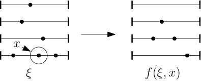 Figure 1
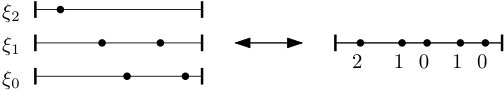 Figure 2
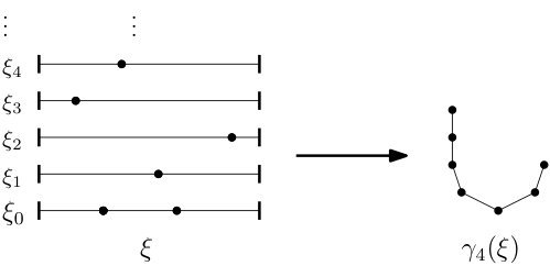 Figure 3
Peer Reviews
No public reviews on file for this paper yet. If you reviewed it on a platform where reviews are public (OpenReview, ICLR, NeurIPS, ICML), you can paste yours below so the community can read it here.
Videos
No videos yet. Explain this paper in a talk, walkthrough, or lecture? Add one.
Taxonomy
TopicsStochastic processes and statistical mechanics · Bayesian Methods and Mixture Models · Data Management and Algorithms
\publicationdetails
212019215628
Expected size of a tree in the fixed point forest
Samuel Regan\affiliationmark1 and Erik Slivken\affiliationmark2 Partially supported by ERC Starting Grant 680275 MALIG
University of California Davis
Dartmouth College
(2019-3-30; 2019-7-16; 2019-9-10)
Abstract
We study the local limit of the fixed-point forest, a tree structure associated to a simple sorting algorithm on permutations. This local limit can be viewed as an infinite random tree that can be constructed from a Poisson point process configuration on . We generalize this random tree, and compute the expected size and expected number of leaves of a random rooted subtree in the generalized version. We also obtain bounds on the variance of the size.
keywords:
sorting algorithms, random trees, Poisson point processes, random permutations
1 Introduction
We start with a simple sorting algorithm on a deck of cards labeled though . If the value of the top card is , place it in the th position from the top in the deck. Repeat until the top card is a . Viewing the deck of cards as a permutation in one-line notation , we create a new permutation, , by removing the value from beginning of the permutation and putting it into position . For example, if then . This induces a graph whose vertices are the permutations of and edges are pairs of permutations Note that has a fixed point at the position
This graph is a rooted forest, which we denote by and call the fixed point forest. A rooted forest is a union of rooted trees, and a tree is a graph that does not contain any closed loops involving distinct vertices. A permutation that begins with 1 is called the base of the tree in which they are contained. A thorough introduction to the fixed point forest can be found in Johnson et al. (2017).
The fixed point forest was first studied in McKinley (2015). The largest tree in has size bounded between and and has as its base the identity permutation. The longest path from a leaf to a base is and is unique, starting from the permutation and ending at the identity.
Let denote the set of permutations of length . For , let denote the collection of fixed points of other than . For each we create a new permutation such that
[TABLE]
We say we bump the value in to create and call a child of . We let denote the set of children of . Every child satisfies hence is connected to in .
Let be the rooted tree in that contains , with designated as the root instead of the unique permutation that starts with in . Let be the subtree of rooted at and consisting of and its descendants, so that We call this the descendant tree of (See Figure 1). Note that for any permutation , there is some such that .
By Theorem 3.5 in Johnson et al. (2017), there exists a tree, , such that as , for chosen uniformly at random from permutations of size , the randomly rooted tree , converges in the local weak sense to . This limiting tree is described in Section 2 of Johnson et al. (2017), and the subtree of which corresponds to the local weak limit of has a similar description, denoted by . In Johnson et al. (2017), they find the distribution for the shortest and longest paths from the root to a leaf in . The main purpose of the paper is to study the size of . For , we define a generalization of , denoted such that . We compute the expected size and expected number of leaves of and show that they are both unbounded for . Finally we find bounds on the second moment of the size of . We show that the second moment has a phase transition from finite to infinite somewhere between and
2 Local limits, point process configurations, and trees
Poisson Point Processes
The following briefly introduces an important probabilistic object: Poisson point processes. A thorough treatment can be found in Kingman (1993).
We say a random variable is if it satisfies If and are two independent and , respectively, then their sum is .
A point process on is an integer-valued measure on Borel sets of . It may be viewed as a collection of points, which represent the atoms of the measure. A point process configuration on is a collection of point processes, each on , and can be viewed as a collection of labelled points on
A Poisson point process on with intensity is a random integer-valued measure which satisfies two properties: For any Borel subset with Borel measure , the number of atoms of the point process in is given by , and for any disjoint Borel subsets of the number of atoms in each are independent. Conditioned on the number of atoms in the location of each of the atoms is independent and uniform in .
Collections of Poisson point processes can be merged to create a single poisson point process. Suppose is a point process on and is point process on with and both independent. Then the union of and is distributed like a point process. The reverse is also true. Let be a point process on and label each atom [math] with probability and otherwise. Let denote the point process consisting of the atoms labeled [math] and the point process of the remaining atoms. Then and are, respectively, independent Poisson() and Poisson() point processes on . This can be generalized further to . If is a Poisson() point process each atom in is independently labeled such that the label is with probability for , then the collection of atoms labeled is a Poisson() point process and each is independent of the rest.
Let and be two independent Poisson( point processes. For , define \xi^{\prime}_{1}=\xi_{2}\big{|}_{[0,x)}+\xi_{1}\big{|}_{(x,1]} to be the point process consisting of the atoms from restricted to the interval and the atoms from restricted to the interval . If is independent of and then the resulting process is also a Poisson() point process.
Weak Convergence
We give a brief definition of the version of local weak convergence that is used to define and . See Aldous and Steele (2004) or Benjamini and Schramm (2001) for a proper discussion of local weak convergence, which is sometimes referred to as Benjamini-Schramm convergence.
Let be a sequence of rooted graphs. For any rooted graph , the -neighborhood of the root, denoted , is the subgraph of induced from all vertices that are distance at most from the root. The rooted graph is the local weak limit of if for every and every finite graph ,
[TABLE]
From point process configurations to trees
Let be a point process configuration on where each is a point process on For each atom define the bump map where
[TABLE]
See Figure 2 for an illustration of this map. Given a point process configuration, , the bump map allows us to recursively define a tree with root whose vertices are point process configurations. Define to be the root of the tree with corresponding point process configuration . Suppose is a vertex in the tree with corresponding point process configuration given by . For each , create a new vertex in the tree with point process configuration given by the bump map . The newly created vertex is a considered a child of . We call this tree the bump tree of and denote it by For fixed let denote the -neighborhood of the root in Only the atoms in are necessary to determine the structure of the , so we may write and assume for . The map is continuous because a slight perturbation of the atoms will not change the relative order of the points in . See Figure 3 for an example of a finite neighborhood of the root of the bump tree for a point process configuration.
For a permutation of length , we say the index or the value is -separated if We define the separation word of point-wise by . No two permutations have the same separation word. From this word we can construct a point process configuration by placing an atom in at position if is a -separated point in .
By Proposition 3.4 in Johnson et al. (2017), for fixed , as tends to infinity,
[TABLE]
where is a point process on . From the arguments of Theorem 3.5 in Johnson et al. (2017), letting , we have by continuity of and the Continuous Mapping Theorem [Billingsley (1999)]. Furthermore, it is seen that is the same as the -neighborhood of the descendant tree with high probability. Therefore is the local weak limit of .
We now can state our main results. For , let be a collection of independent point processes on and let be the corresponding bump tree of . Let denote the number of vertices and the number of leaves in Finally let and denote the expectation and probability associated with point processes. We now may state our main results.
Theorem 1**.**
For , , and diverges.
Theorem 2**.**
For , , and diverges.
Theorem 3**.**
For , diverges. For , is finite.
3 Comparison with Galton-Watson trees
In this section we compare our results to the well-studied Galton-Watson tree Watson and Galton (1875); Neveu (1986).
A Galton-Watson tree, , can be constructed through a simple random process. Start with a root and a nonnegative integer-valued random variable . Create children of where is distributed as and independent copy of . For each child, , of repeat this process, where is an independent copy of . Depending on the distribution of , the resulting tree will have drastically different behavior.
Fix a nonnegative integer-valued random variable with finite expectation and finite second moment Let . Let denote the number of children of the root of and for , let denote the number of vertices in the subtree consisting of the th child and all of its descendants. Each is distributed identically as an independent copy of . We denote the size of conditioned on by . Taking expectation we have and thus
[TABLE]
and so
[TABLE]
A similar approach for the second moment gives the equation
[TABLE]
which can be simplified to
[TABLE]
Given that and is finite, (1) shows that finite. In particular if is then agrees with from Theorem 1, while Theorem 3 shows the second moment cannot agree with the second moment if since the former is finite while the latter diverges.
The approach used to compute and cannot be used to compute and because the subtrees from the root in are not independent of each other.
4 Words from point process configurations
For a collection of point processes on , , let be the word constructed from the relative order of the atoms in . For example see Figure 4. Assuming that no two atoms of are in the same location, the structure of the -neighborhood of the root in the tree can be constructed directly from this word. Let denote the space of finite words with letters from .
If is a point process configuration, this induces a probability measure on for every . The following lemma describes this distribution.
Lemma 4**.**
Let be a point process configuration and the word given by the relative order of the first point processes of . Let denote a fixed word of length in . Then
[TABLE]
and
[TABLE]
Proof.
Construct the independent point processes from a single point process by labeling each atom independently from , choosing the label uniformly at random. The probability that is precisely the probability that a point process has atoms in , the right hand side of (2). As the labeling is independent for each atom, each of the possible labelings is equally likely, so the probability that for a fixed of length is computed by dividing the right hand side of (2) by , giving (3). ∎
For of length we write in one line notation. For a fixed subset of indices let . We may refine Lemma 4 even further.
Lemma 5**.**
Let be a word in . Let , and be a set of indices such that . Then,
[TABLE]
Proof.
Conditioned on , the labels of the atoms indexed by are chosen independently so
[TABLE]
and the statement follows. ∎
The tree with word will agree up to a relabeling of the vertices of the tree if A vertex in the tree corresponds to bumping a particular set of atoms in a particular order. Therefore the measure on words in is exactly the measure we need to understand the .
We can translate our language of bumping atoms in to bumping letters in words. Let . For each , we construct a new word by removing the chosen [math] and reducing every letter to the left of it by We say the index of this letter [math] is bumped and indices less than the bumped index are shifted. The set of indices of the [math]s in a word are called the bumpable indices. The set of words that can be constructed by bumping a single [math] in are called the children of and denoted For example the word has has two children, and , where is used to indicate bumped indices or indices shifted below zero. Once the letter at an index becomes in a word it can never become [math] in one of its descendants. We construct a rooted tree, denoted , following a process that mirrors our construction of for point process configurations. We let denote the -neighborhood of the root in .
We may omit the symbol in the labeling of the tree. The symbol is used to emphasize that the set of indices is the same for each word in the same tree. See Figure 5 for the rooted tree in associated with the word . The sequence of indices that are bumped to reach the vertex in is called the bumping sequence of .
For and every vertex there is a corresponding set of atoms that must be bumped in a particular order to reach . This sequence of atoms induces an ordered set of indices and permutation, , of length such that is obtained by bumping the atoms at the indices in order where each of the indices must be [math] when they are bumped. We say the set of indices reaches by the order . Since is a tree, any such is reachable by a unique pair .
For a set of indices , we say is complete in if there exists an order and a sequence of words such that for , is obtained by bumping the index in . Whether or not is complete in is independent of the letters not in . The following lemma gives conditions on when is complete in .
Lemma 6**.**
If is complete in with , there is a unique such that a vertex in is reachable by . If , then for each there is a unique sequence of values such if then there exists a vertex in that is reachable by .
Finally, is complete with respect to if and only if for .
Proof.
Since is complete in there is at least one and in such that is reachable by . First is bumpable if and only if In order for to be bumpable after bumping up to , the label of must be [math], and therefore index must be shifted exactly times by bumping indices larger then For this to occur there must be exactly integers such that and In terms of we have for ,
[TABLE]
The sequence of values is the unique inversion table (Knuth (1998)) for the permutation . No two permutations have the same inversion table and thus must be unique. Given a , if is the inversion table for then will be complete with respect to .
Finally we have that is an inversion table if and only if for . We also have that by definition. ∎
Define the following truncated factorial function:
[TABLE]
Note that .
Let denote the set of subwords of length such such that is complete in if and only if . For any and , by Lemma 6,
[TABLE]
and for , this simplifies to
[TABLE]
5 Expectation of and
Let denote the number of vertices in . Let denote the number of leaves in that are distance less than from the root. Note that a leaf in that is distance from the root may not be a leaf in By Theorem 5.1 in Johnson et al. (2017), the longest path to a leaf in is almost surely finite and therefore is identical to for large enough To compute the expectation of and it suffices to compute the expectation of and and let tend to infinity.
Let be chosen from . For let Similarly let denote the set of leaves in , so that for , , the number of leaves in exactly distance from the root. By linearity of expectation
[TABLE]
and
[TABLE]
For a fixed , let be the set of all subsets of indices . Consider a fixed and a word of length with letters less than . If a word has length , there are possible fillings of the indices in and there are ways to fill the indices of so that is complete in .
By Lemma 5 we have
[TABLE]
By the one-to-one correspondence with complete indices in of size with vertices in exactly distance from the root, the expectation of is
[TABLE]
For ,
[TABLE]
and , so
[TABLE]
of Theorem 1.
From (7), for and . Then and by Monotone Convergence Theorem
[TABLE]
∎
Expected number of leaves
For a set of indices of size that are complete in , let denote the word obtained after bumping every index in . The vertex labelled with is a leaf if it contains no bump-able indices, that is has no [math]s. Let and For , an index is bump-able in if and only if If and , and hence cannot be bump-able. Otherwise if , there are choices for so that is not bump-able.
Let denote the number words, of length in such that corresponds to a leaf in . There are possible ways to fill in the indices of . For ,
[TABLE]
For this simplifies to
[TABLE]
Thus for we have
[TABLE]
For the expectation of is
[TABLE]
Summing over gives
[TABLE]
of Theorem 2.
From (12), for and . Then and by Monotone Convergence Theorem
[TABLE]
∎
6 Expectation of
For let . Let be the set of all ordered pairs of subsets of , , such that , , and and let . We denote the set of distinct subwords on the indices such that and both and are complete by . The size of is denoted by and only depends on the relative order of and . Suppose . For both subwords to be complete, each index must have letters strictly less than , each index must have letters strictly less than , and each index must have letters strictly less than . Thus
[TABLE]
The following lemma provides uniform bounds of for all .
Lemma 7**.**
Fix and . For , if , then
[TABLE]
Otherwise if , then
[TABLE]
Proof.
For a fixed and , will reach its minimum value over when the product in the denominator is maximized in the right hand side of (14). The denominator of is maximized when every index in is less than every index in so . In this case for the denominator of the right hand side of (14) is given by
[TABLE]
and
[TABLE]
Otherwise for
[TABLE]
For the other direction is maximized when the denominator in the right-hand side of (14) is minimized. This occurs when every index in is greater than every index in . In this case,
[TABLE]
These bounds on will give us bounds on Let For a fixed set of indices let denote the indicator function that is if is complete and [math] if is not complete or is not a subset of indices of . Then
[TABLE]
with . We also have
[TABLE]
For a fixed pair , using Lemma 5 we have
[TABLE]
The value of depends on but the upper and lower bounds from Lemma 7 only depend on and . Thus we have bounds of (16) that are uniform for all . For each the size of is . Thus
[TABLE]
Summing over in (17) gives the lower bound
[TABLE]
Similarly for the upper bound we have
[TABLE]
of Theorem 3.
In this section we make repeated use of the identity
[TABLE]
See Wilf (2006) for a variety of similar identities.
By Fatou’s Lemma so
[TABLE]
The right hand side of (20) can be simplified further. Suppose Then
[TABLE]
There is an issue when in (22) and (23). But in this case in (21), so (22) becomes which is finite. Otherwise (23) diverges precisely when which occurs if For the other direction we have
[TABLE]
The last line (24) converges when which occurs when ∎
As increases from to a phase transition occurs where becomes infinite. With a more precise analysis of the size of that depends more closely on the relative order of and , one might be able to obtain the exact location where this phase transition occurs.
Acknowledgements
We wish to express thanks to Tobias Johnson and Anne Schilling for useful discussions.
The reference list from the paper itself. Each links out to its DOI / PubMed record.
- 1Aldous and Steele (2004) D. Aldous and J. M. Steele. The objective method: probabilistic combinatorial optimization and local weak convergence. In Probability on discrete structures , volume 110 of Encyclopaedia Math. Sci. , pages 1–72. Springer, Berlin, 2004. 10.1007/978-3-662-09444-0_1 . URL http://dx.doi.org/10.1007/978-3-662-09444-0_1 . · doi ↗
- 2Benjamini and Schramm (2001) I. Benjamini and O. Schramm. Recurrence of distributional limits of finite planar graphs. Electron. J. Probab. , 6:no. 23, 13 pp. (electronic), 2001. ISSN 1083-6489. 10.1214/EJP.v 6-96 . URL http://dx.doi.org/10.1214/EJP.v 6-96 . · doi ↗
- 3Billingsley (1999) P. Billingsley. Convergence of probability measures . Wiley Series in Probability and Statistics: Probability and Statistics. John Wiley & Sons, Inc., New York, second edition, 1999. ISBN 0-471-19745-9. 10.1002/9780470316962 . URL http://dx.doi.org/10.1002/9780470316962 . A Wiley-Interscience Publication. · doi ↗
- 4Johnson et al. (2017) T. Johnson, A. Schilling, and E. Slivken. Local limit of the fixed point forest. Electron. J. Probab. , 22:Paper No. 18, 26, 2017. ISSN 1083-6489. 10.1214/17-EJP 36 . URL https://doi.org/10.1214/17-EJP 36 . · doi ↗
- 5Kingman (1993) J. F. C. Kingman. Poisson processes , volume 3 of Oxford Studies in Probability . The Clarendon Press, Oxford University Press, New York, 1993. ISBN 0-19-853693-3. Oxford Science Publications.
- 6Knuth (1998) D. E. Knuth. The Art of Computer Programming, Volume 3: (2Nd Ed.) Sorting and Searching . Addison Wesley Longman Publishing Co., Inc., Redwood City, CA, USA, 1998. ISBN 0-201-89685-0.
- 7Mc Kinley (2015) G. Mc Kinley. A problem in card shuffling, UC Davis Undergraduate Thesis, 2015. https://www.math.ucdavis.edu/files/1114/3950/6599/Mc Kinley_UG_Thesis_SP 15.pdf .
- 8Neveu (1986) J. Neveu. Arbres et processus de Galton-Watson. Ann. Inst. H. Poincaré Probab. Statist. , 22(2):199–207, 1986. ISSN 0246-0203. URL http://www.numdam.org/item?id=AIHPB_1986__22_2_199_0 .