Fiend -- Finite Element Quantum Dynamics
Janne Solanp\"a\"a, Esa R\"as\"anen

TL;DR
Fiend is a Python-based simulation package for solving the 3D time-dependent Schrödinger equation in cylindrically symmetric systems, enabling detailed studies of electron dynamics under complex electromagnetic fields with advanced numerical methods.
Contribution
It introduces a finite element method-based solver with full minimal coupling for inhomogeneous vector potentials, supporting flexible and accurate quantum dynamics simulations.
Findings
Supports inhomogeneous vector potentials beyond dipole approximation
Uses FEM for spatial discretization and advanced time-stepping methods
Provides user-friendly API with extensive documentation
Abstract
We present Fiend - a simulation package for three-dimensional single-particle time-dependent Schr\"odinger equation for cylindrically symmetric systems. Fiend has been designed for the simulation of electron dynamics under inhomogeneus vector potentials such as in nanostructures, but it can also be used to study, e.g., nonlinear light-matter interaction in atoms and linear molecules. The light-matter interaction can be included via the minimal coupling principle in its full rigour, beyond the conventional dipole approximation. The underlying spatial discretization is based on the finite element method (FEM), and time-stepping is provided either via the generalized-{\alpha} or Crank-Nicolson methods. The software is written in Python 3.6, and it utilizes state-of-the-art linear algebra and FEM backends for performance-critical tasks. Fiend comes along with an extensive API documentation,…
Click any figure to enlarge with its caption.
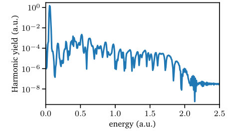 Figure 1
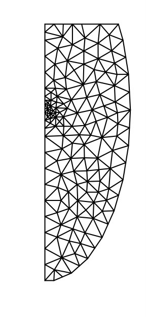 Figure 2
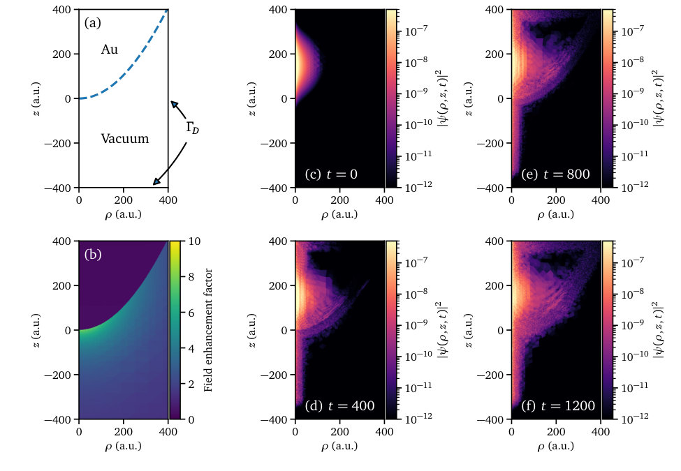 Figure 3
Peer Reviews
No public reviews on file for this paper yet. If you reviewed it on a platform where reviews are public (OpenReview, ICLR, NeurIPS, ICML), you can paste yours below so the community can read it here.
Videos
No videos yet. Explain this paper in a talk, walkthrough, or lecture? Add one.
Taxonomy
TopicsStrong Light-Matter Interactions · Photonic and Optical Devices · Quantum and electron transport phenomena
Fiend – Finite Element Quantum Dynamics
J. Solanpää
E. Räsänen
Computational Physics Laboratory, Tampere University, Tampere FI-33101, Finland
Abstract
We present Fiend – a simulation package for three-dimensional single-particle time-dependent Schrödinger equation for cylindrically symmetric systems. Fiend has been designed for the simulation of electron dynamics under inhomogeneous vector potentials such as in nanostructures, but it can also be used to study, e.g., nonlinear light-matter interaction in atoms and linear molecules. The light-matter interaction can be included via the minimal coupling principle in its full rigour, beyond the conventional dipole approximation. The underlying spatial discretization is based on the finite element method (FEM), and time-stepping is provided either via the generalized- or Crank-Nicolson methods. The software is written in Python 3.6, and it utilizes state-of-the-art linear algebra and FEM backends for performance-critical tasks. Fiend comes along with an extensive API documentation, a user guide, simulation examples, and allows for easy installation via Docker or the Python Package Index.
keywords:
Time-dependent Schrödinger equation, finite element method, atoms, nanostructures, light-matter interaction, strong field physics
††journal: Computer Physics Communications
**PROGRAM SUMMARY
** Program Title: Fiend
Journal Reference:
Catalogue identifier:
Licensing provisions: MIT License
Programming language: Python 3.6
Computer: Tested on x86_64 architecture.
Operating system: Tested on Linux and macOS.
RAM: Simulation dependent: from megabytes to hundreds of gigabytes.
Parallelization: MPI-based parallelization. Thread-based parallelization via BLAS and LAPACK backends.
Classification: 2.2 Spectra, 2.5 Photon Interactions, 4.3 Differential equations, 6.5 Software including Parallel Algorithms
External routines/libraries:
PETSc, SLEPc, FEniCS, HDF5
petsc4py, slepc4py, mpi4py, h5py, numpy, scipy, matplotlib, psutil, mypy, progressbar2
*Nature of problem:
*Solution of time independent and time dependent single active electron Schrödinger equations in cylindrically symmetric systems including interactions with spatially inhomogeneous vector potentials.
*Solution method:
*Finite element discretization of the Schrödinger equation. Time evolution via the generalized- or Crank-Nicolson methods.
*Restrictions:
*Cylindrically symmetric single active electron systems.
*Unusual features:
*Finite element discretization of the equations allowing inhomogeneous spatial dependence of the vector potential (e.g., plasmon-enhanced fields). Integration with the FEniCS finite element suite. Installable from the Python Package Index. Pre-installed Docker images available.
*Additional comments:
*The source code is also available at https://fiend.solanpaa.fi.
Python package available at https://pypi.org/project/fiend/.
Docker images are available at https://hub.docker.com/r/solanpaa/fiend/.
*Running time:
*From minutes to weeks, depending on the simulation.
1 Introduction
Simulation of three-dimensional (3D) single particle quantum mechanics (QM) is still one of the most used computational approaches in the strong field and attosecond communities. In these fields, the nonlinear interaction of the atomic or molecular electron with the driving laser field requires fast and accurate integration of the 3D time dependent Schrödinger equation (TDSE). Recent applications include, e.g., benchmarking of approximate models [1, 2, 3, 4, 5, 6], study of high-order harmonic generation [7, 8, 9], and the study of photoionization [10, 11, 12, 13, 14].
Recently the strong-field and attosecond communities have turned their attention to related phenomena in nanostructures. There the nanostructure geometry and plasmonic effects cause the electromagnetic field to become extremely inhomogeneous [15] which, in turn, causes significant differences to the traditional ultrafast and strong-field phenomena in atoms and molecules. Recent studies include, e.g., nanostructure-enhanced photoionization of gases [16, 17, 18] and electron emission from nanostructures such as tips [19, 20, 21, 22, 23, 24, 25, 26, 27, 28] and rods [29, 30, 31, 32, 33].
There are already multiple software designed for integrating the three-dimensional time-dependent Schrödinger equation (TDSE). Open-source software include, e.g., Qprop [34], Octopus [35, 36], QnDynCUDA [37], and WavePacket [38], but there are also plenty of other options such as SCID-TDSE [39], tRecX [40, 41], and ALTDSE [42]. Qprop, SCID-TDSE, and QnDynCUDA solve the TDSE using a grid-based representation of the radial coordinates and spherical harmonics for the angular dependence; TRecX and WavePacket support multiple basis sets; Octopus relies on a real-space grid; and ALTDSE requires end-user to provide the matrices in an appropriate eigenbasis.
However, efficient and accurate simulation of ultrafast and strong-field phenomena in nanostructures and nanostructure-enhanced gases requires specialized TDSE-solvers. Most importantly, since the laser electric field has strong spatial inhomogeneity, it is imperative to have position-dependent control of simulation accuracy. In addition, it would be beneficial to have the TDSE-solver directly interface with a solver for the electromagnetic problem.
To this end, we have developed Fiend, a QM simulator based on finite element method (FEM). Fiend provides solvers for the time independent and time-dependent single active electron Schrödinger equations in cylindrically symmetric systems111Although the restriction to cylindrically symmetric systems can be lifted relatively easily if needed. for solving time-independent and time-dependent Schrödinger equations in cylindrically symmetric systems. We have designed Fiend to integrate with the open source FEniCS finite element suite [43, 44, 45, 46, 47, 48, 49] allowing for easy description of complicated system geometries. Being FEM-based, Fiend also allows the use of potentials with integrable singularities.
Fiend is written in Python 3.6, but much of the heavy number-crunching is delegated to well-tested and efficient external libraries. The software is modular and easy to extend. We also provide a comprehensive unit- and integration-test suite to ensure reliability. Moreover, we provide straightforward installation methods either via the Python Package Index [50] or as Docker images [51].
This paper is organized as follows. In Sec. 2 we describe the finite element discretization of the Schrödinger equations and the time-propagation schemes. Section 3 focuses on the design and implementation of Fiend. Section 4 provides a few example simulation, and finally, in Sec. 5 we summarize this paper and possible extensions of the presented software suite.
2 Finite element quantum mechanics
2.1 Systems
Fiend is designed for simulating cylindrically symmetric single (active) electron systems interacting with time and (optionally) position dependent vector potentials. The Hamiltonian operator of these systems can be written as
[TABLE]
where is the planar radial coordinate operator, the -coordinate operator, the kinetic energy operator with respect to planar radial motion222 Note that is not proportional to the square of the planar radial momentum operator, i.e.,
\begin{split}\hat{T}_{\rho}&=-\frac{1}{2}\left(\frac{\partial^{2}}{\partial_{\rho}^{2}}+\frac{1}{2}\frac{\!\partial}{\partial_{\rho}}\right)\\ &\neq\frac{1}{2}\left[-{\mathrm{i}\mkern 1.0mu}\left(\frac{\!\partial}{\partial_{\rho}}+\frac{1}{2\rho}\right)\right]^{2}=\frac{\hat{p}_{\rho}^{2}}{2}.\end{split}
(2)
This is a peculiarity of quantum mechanics in cylindrical coordinates [52]., the -component of the momentum operator, the static potential, and the light-matter interaction operator.
Fiend readily supports three types of interaction operators . First, for linearly polarized vector potentials in the length gauge the interaction operator is given by
[TABLE]
secondly, in the velocity gauge the interaction operator reads
[TABLE]
and finally for more general cylindrically symmetric inhomogeneous vector potentials we provide the interaction operator
[TABLE]
Moreover, Fiend supports all interaction operators of the form .
The above interaction operators conserve the magnetic quantum number , and by default, we simulate only the subspace. Correspondingly, the coordinate space domain is a two-dimensional slice of the cylindrical coordinates, , which we truncate for numerical simulations to a finite domain [see Fig. 1(a)].
2.2 Time independent Schrödinger equation
On the domain the time-independent Schrödinger equation (TISE) can be written as
[TABLE]
where is the th eigenpair. This equation is accompanied by continuity boundary condition at ,
[TABLE]
Elsewhere on the boundary we can choose freely between zero Neumann boundary conditions (ZNBCs) and zero Dirichlet boundary conditions (ZDBCs) – depending on the requirements of our model. For example, in Fig. 1(a) where we have imposed ZNBC on the upper boundary of the simulation domain, , and ZDBC on the arc .
To discretize TISE, we begin by looking for eigenpairs of the weak form corresponding to Eq. (6) and the boundary conditions described above. The weak form is given by
[TABLE]
where is the standard Sobolev space on of real-valued -integrable functions with integrable first derivatives. Notice also that includes ZDBCs, and the natural inner product is
[TABLE]
Furthermore, we must restrict ourselves to a finite dimensional approximation of . First, the simulation domain is described using an unstructured triangular mesh which supports arbitrary refinement [see, e.g., Fig. 1(b)]. Next, we construct a basis of continuous low-order Lagrange polynomials , each with compact support on the mesh elements. This basis spans a finite dimensional function space
[TABLE]
where the TISE weak form [Eq. (8)] can be written as a finite dimensional generalized Hermitian eigenvalue equation
[TABLE]
Here is a vector of the real-valued expansion coefficients of the th eigenstate, the corresponding eigenvalue, and
[TABLE]
are the overlap, kinetic energy, and potential energy matrices, respectively. Note that since the static potential of the system is implemented only via Eq. (14) which involves integration, we can use any static potential for which Eq. (14) is finite, e.g., the Coulomb potential.
2.3 Time dependent Schrödinger equation
In a similar manner as with TISE, TDSE can be discretized as
[TABLE]
where is a vector of the complex-valued expansion coefficients of the wave function . , , and are constructed the same way as for TISE (except we add an imaginary absorbing potential to ), and the light-matter interaction matrix is given by
[TABLE]
The basis of the discrete function space for TDSE can, in general, be different from the one used for TISE. This is useful in practice since often the stationary states can be computed in a much smaller simulation domain than needed for an accurate description of the TDSE. We can change the function space by three methods: (1) using a larger simulation domain for the TDSE, (2) refining the mesh according to the requirements of the TDSE simulation, and (3) change the degree of our basis functions according to the required accuracy.
For evolving the discretized state, i.e., the expansion coefficients according to Eq. (15), Fiend implements two approximations of the time evolution operator: the Crank-Nicolson (CN) method [53] and the generalized- method [54].
The Crank-Nicolson method can be written as
[TABLE]
and it is a unitary time-reversible transformation [53] as long as the matrix inversion is performed to a sufficient accuracy.
The generalized- method was originally developed for integrating the equations of motion arising from fluid dynamics [54], but we have successfully applied it to the TDSE integration. To the best of our knowledge, the -method has not been proven to be unitary nor is it exactly time-reversible. Nevertheless, we have achieved accuracies comparable to the CN method – and in the case of extremely inhomogeneous vector potentials, the generalized- method seems to be significantly more stable than CN.
2.4 Incorporation of boundary conditions
The continuity boundary condition at and ZNBCs are automatically included by dropping the boundary integrals when deriving Eqs. (8) and (13). However, the ZDBCs must be included in the system matrices via the following modifications: the rows and columns of , , , and corresponding to the degrees of freedom (DOFs) on the boundary with ZDBCs set to zero. Only for we must set the corresponding diagonal elements to one to ensure invertibility. Note that it’s crucial to zero out not only the rows but also the corresponding columns of the matrices to retain hermiticity.
Embedding ZNBCs via the vanishing boundary terms when deriving Eqs. (8) and (13) causes a practical issue: Some operators such as , , and become non-Hermitian. Minor adjustments at the boundaries can remedy this, namely,
[TABLE]
where is the outwards facing unit normal on the simulation domain boundary at point . This trick has been previously used to obtain the correct Hermitian operators in hyperspherical coordinates [52].
Another aspect to consider is the weak enforcement of ZNBCs compared to ZDBCs. If there was significant electron density on the Neumann boundary , it will start to oscillate and eventually violate the ZNBC. This can be remedied when operating with matrix inverses as in the second step of the CN-propagator. We can add an extra error term, e.g., of the form
[TABLE]
to the error estimator in our numerical implementation. This will remove – or at least lessen – the issue arising from the weak enforcement of ZNBCs.
3 Implementation
3.1 Overview
We have implemented finite element discretization of TISE and TDSE in the Python software package Fiend following the recipes of Sec. 2. Fiend is written in Python 3.6 and it utilizes reliable libraries commonly pre-installed in high-performance clusters and supercomputers. For sparse linear algebra we use the Portable, Extensible Toolkit for Scientific Computation (PETSc) [55, 56, 57] and the Scalable Library for Eigenvalue Problem Computations (SLEPc) [58, 59]. Meshing and other standard FEM-related parts are built on top of the components of the FEniCS project [43, 44, 45, 46, 47, 48, 49], and filesystem IO is largely based on HDF5 [60] via h5py [61, 62]. In postprocessing and visualization we use also numpy [63], scipy [64], and matplotlib [65]. Fiend is parallelized using MPI via mpi4py [66, 67, 68].
The PETSc-dependency is slightly complicated as PETSc needs to be compiled either with real number support (x)or with complex number support. Fiend, on the other hand, needs real numbers for TISE and post-processing but complex numbers for propagation. Consequently, the user must install both the real and complex versions of PETSc/SLEPc stacks and switch between these for different simulation steps. This factitious requirement for two different installations of PETSc can be revisited in the future upon the completion of DOLFIN-X [69] and FFC-X [70] including the merge of complex number support in FEniCS [71],
To ease installation, we provide a Docker [51] container with Fiend and all its dependencies preinstalled, see https://hub.docker.com/r/solanpaa/fiend/ for more details. In the same spirit, Fiend is also available in the Python Package Index [50] and can be installed with pip [72].
3.2 Library usage and numerical methods
A typical usage of the Fiend suite is demonstrated in Fig. 2. First we solve the TISE to obtain a set of stationary states. This includes meshing the domain for the time independent simulation and assembling the system matrices (12)–(14) with appropriate boundary conditions (see Sec. 2.4).
The TISE eigenproblem, Eq. (11), is solved (by default) with Rayleigh Quotient Conjugate Gradient (RQCG) method combined with classical Gram-Schmidt orthogonalization of the Krylov subspace basis with adaptive iterative refinement for increased numerical stability. RQCG is a variational method which essentially minimizes the Rayleigh quotient
[TABLE]
of a desired number of orthonormal vectors with respect to the bilinear product induced by [59]. Upon convergence, this corresponds to smallest real eigenpairs of TISE.
Step 2 (see Fig. 2) is to prepare the discrete description of the TDSE. This includes meshing the domain for the time dependent problem, interpolating stationary states to the new mesh, and also assembly of the system matrices (12)–(14) and the time-independent part(s) of Eq. (16).
The propagation in Step. 3 (Fig. 2) requires the user to load the environment with complex number PETSc. The time-dependent Hamiltonian is constructed from the matrices computed in the previous step, and the discrete TDSE (15) is solved with PETSc’s propagators. We also provide code templates for easy implementation of new propagators.
Finally, we provide a set of example scripts for postprocessing. These scripts include, e.g., visualization of the integrated electron density in time and temporal shape of the laser field, but there are also scripts to compute more complex observables such as the high-harmonic and photoelectron spectra.
All the numerical methods in Fiend depend on efficient sparse linear algebra operations implemented in PETSc. By default, matrix inversions and the solution of linear equations are carried out with Generalized Minimal RESidual method (GMRES) [73], where the convergence criterion is computed with respect to the norm induced by the inner product in Eq. (9). Unfortunately, the PETSc linear algebra backend does not allow us to build the basis of the Krylov subspace with respect to a custom inner product. However, we have found the basis built with the standard Hermitian inner product to be sufficient performance-wise. Direct solvers such as SuperLU_DIST [74, 75, 76] and MUMPS [77, 78] are supported only with matrices that can be explicitly constructed without too high cost.
3.3 Note on meshing
We provide a way to generate meshes with arbitrary refinement in the coordinate space. The user should supply a function returning the maximum allowed cell circumradius333Radius of the smallest circle enclosing the given triangular cell. at coordinate , and the mesh can be refined until all cells of the mesh have circumradius below the desired one.
By default, the maximum cell circumradius is given by [79]
[TABLE]
For the cell circumradii are below , and as , the maximum cell circumradius increases monotonically to .
4 Examples and test cases
4.1 Field-free propagation
To assess the stability and accuracy of the numerical methods implemented in Fiend, we compute a field-free propagation of an electron prepared in a superposition of Hydrogen 1s and 2s states,
[TABLE]
This state is propagated up to of time. The simulation domain up to is meshed using the default refinement introduced in Sec. 3.3 with , , and We assess the accuracy of the numerical solution by comparing the simulated state to the exact result:
[TABLE]
The stability is investigated by evaluating how much the norm of the state differs from unity, i.e.,
[TABLE]
Both the -propagator and the CN propagator reach an accuracy of 0.00524 % for the overlap with the time-step , and the norm of the simulated state deviates from unity only by . This demonstrates the applicability of the propagators for the simulation of FE-discretized TDSE in cylindrical coordinates.
4.2 High-harmonic generation
Next we demonstrate the applicability of Fiend to simulate high-order harmonic generation (HHG). According to the three-step model [80, 81], an atomic electron is excited to continuum and driven to oscillate around the atom [82]. Upon recombination with the parent ion, the excess energy is released as high-energy photons.
Full 3D simulation of HHG via TDSE is a difficult task due to the long extent of the electron wave function when driven by a short laser pulse. In order to obtain a decent description of the single-atom response for HHG, a large simulation domain is needed. We setup a simulation domain of radius with a more refined mesh at the origin and gradually sparser mesh for larger radii.
The intensity spectrum of the single-atom response is proportional to the square of the Fourier transform of the dipole acceleration [83],
[TABLE]
where we compute the dipole acceleration via Ehrenfest’s theorem [84], i.e.,
[TABLE]
In Fig. 3 we show the computed high-order harmonic spectrum computed for a hydrogen atom under a laser pulse with carrier frequency corresponding to , intensity full width at half maximum , and electric field peak intensity . The spectrum is a typical HHG spectrum from a femtosecond laser pulse, and it ends at the cut-off energy in a decent agreement with the three-step model’s cutoff [80, 81].
4.3 Metal nanotips and inhomogeneous fields
Metal nanotips have recently attracted attention due to their ability to enhance the laser electric field at the tip apex via plasmonic effects (see, e.g., [19, 20, 21, 22, 23, 24, 25, 26, 27, 28]). Fiend is capable of computing single-electron dynamics of these metal nanotapers including correctly the interaction with the inhomogeneous plasmon enhanced laser field.
The first step is to compute the plasmon enhanced near field. Here we consider a gold nanotip with apex radius and full opening angle of as demonstrated in Fig. 4(a). For typical laser wavelengths, such as used here, a quasistatic description of the laser vector potential is applicable, i.e.,
[TABLE]
where the spatial form is the same as for the electric field
[TABLE]
The electrostatic potential can be computed from the Poisson equation
[TABLE]
where is the dielectric function of the material at position . Inside the gold nanotip the complex dielectric function (at ) is [85, 86] and at vacuum .
We can describe Eq. (31) using cylindrical coordinates. The interface condition
[TABLE]
gives rise to the weak form
[TABLE]
with the test function space
[TABLE]
and the trial function space
[TABLE]
The simulation domain is a rectangular area, and the ZDBCs described above are imposed on the external boundaries denoted by . Note that Fig. 4(a) demonstrates the domain and boundaries for the quantum simulation – for Poisson equation we employ a much larger simulation domain. The equation (31) can be solved easily with the FEniCS FEM-suite and we provide an example script at demos/nanotip/1_near_field.py
The computed spatial distribution of the field, , is demonstrated in Fig. 4(b). The field is at its maximum at the nanotip apex and decays rapidly with the distance to the tip. We note that this quasistatic solution provides field-enhancement factor of which is comparable with experimental results [87].
In TDSE, we use a potential well for the static potential,
[TABLE]
where 5.31\text{,}\mathrm{e}\mathrm{V}$$ is the work function of Au (111)-surface [88].
We prepare the electron as a Gaussian wave packet [Fig. 4(c)] and assemble the system matrices – including the inhomogeneous field – with demos/nanotip/3_prepare_tdse.py. The preparation step is slightly more complex than for linearly polarized vector potentials, but the provided example script should work as a template for further expansions.
We use a pulse with full width at half maximum for the Gaussian envelope. The maximum electric field amplitude without nanostructure enhancement is set to . Snapshots of the electron density during propagation are shown in Figs. 4(c)-(f). As expected, the electron emission is concentrated at the tip apex where the field enhancement is at its highest. Only a small percentage (\sim$$2 %) of the electron density is absorbed at the simulation box boundary.
5 Summary
We have presented Fiend – a versatile solver for single-particle quantum dynamics in cylindrically symmetric systems. This Python package provides an easy path for the study of nonlinear strong-field phenomena in atoms and nanostructures under both homogeneous and inhomogeneous vector potentials. Moreover, the finite element discretization used by Fiend can adapt to complicated system geometries. The package is parallelized using MPI, and much of the high-performance computing is delegated to state-of-the-art numerical libraries. Fiend is modular and easy to extend, and we provide comprehensive documentation for the program code.
We have demonstrated the capabilities of Fiend by simulating two different scenarios. The simulation of high-order harmonic generation from a laser-driven hydrogen atom shows that Fiend can be applied to traditional strong-field phenomena in atoms. Furthermore, a simulation of the photoionization of a gold nanotip demonstrates Fiend’s suitability for studying plasmon-enriched strong-field phenomena in nanostructures.
Acknowledgements
We are grateful to Matti Molkkari and Joonas Keski-Rahkonen for insightful discussions. This work was supported by the Alfred Kordelin foundation and the Academy of Finland (grant no. 304458). We also acknowledge CSC – the Finnish IT Center for Science – for computational resources.
The reference list from the paper itself. Each links out to its DOI / PubMed record.
- 1[1] N. Suárez, A. Chacón, J. A. Pérez-Hernández, J. Biegert, M. Lewenstein, M. F. Ciappina, High-order-harmonic generation in atomic and molecular systems, Phys. Rev. A 95 (2017) 033415. doi:10.1103/Phys Rev A.95.033415 . · doi ↗
- 2[2] N. I. Shvetsov-Shilovski, M. Lein, L. B. Madsen, E. Räsänen, C. Lemell, J. Burgdörfer, D. G. Arbó, K. Tőkési, Semiclassical two-step model for strong-field ionization, Phys. Rev. A 94 (2016) 013415. doi:10.1103/Phys Rev A.94.013415 . · doi ↗
- 3[3] A. Galstyan, O. Chuluunbaatar, A. Hamido, Y. V. Popov, F. Mota-Furtado, P. F. O’Mahony, N. Janssens, F. Catoire, B. Piraux, Reformulation of the strong-field approximation for light-matter interactions, Phys. Rev. A 93 (2016) 023422. doi:10.1103/Phys Rev A.93.023422 . · doi ↗
- 4[4] M. Klaiber, J. c. v. Daněk, E. Yakaboylu, K. Z. Hatsagortsyan, C. H. Keitel, Strong-field ionization via a high-order coulomb-corrected strong-field approximation, Phys. Rev. A 95 (2017) 023403. doi:10.1103/Phys Rev A.95.023403 . · doi ↗
- 5[5] A.-T. Le, H. Wei, C. Jin, C. D. Lin, Strong-field approximation and its extension for high-order harmonic generation with mid-infrared lasers, Journal of Physics B: Atomic, Molecular and Optical Physics 49 (5) (2016) 053001. doi:10.1088/0953-4075/49/5/053001 . · doi ↗
- 6[6] S. Majorosi, M. G. Benedict, A. Czirják, Improved one-dimensional model potentials for strong-field simulations, Phys. Rev. A 98 (2018) 023401. doi:10.1103/Phys Rev A.98.023401 . · doi ↗
- 7[7] L. Wang, G.-L. Wang, Z.-H. Jiao, S.-F. Zhao, X.-X. Zhou, High-order harmonic generation of li + with combined infrared and extreme ultraviolet fields, Chinese Physics B 27 (7) (2018) 073205. doi:10.1088/1674-1056/27/7/073205 . · doi ↗
- 8[8] Z. Abdelrahman, M. A. Khokhlova, D. J. Walke, T. Witting, A. Zair, V. V. Strelkov, J. P. Marangos, J. W. G. Tisch, Chirp-control of resonant high-order harmonic generation in indium ablation plumes driven by intense few-cycle laser pulses, Opt. Express 26 (12) (2018) 15745–15758. doi:10.1364/OE.26.015745 . · doi ↗