Deep neural networks algorithms for stochastic control problems on finite horizon: numerical applications
Achref Bachouch, C\^ome Hur\'e, Nicolas Langren\'e, Huyen Pham

TL;DR
This paper evaluates deep learning algorithms for high-dimensional stochastic control problems, demonstrating their effectiveness through numerical experiments on PDEs, financial, and energy storage applications, with comparisons to existing methods.
Contribution
It introduces and tests deep neural network algorithms for solving complex stochastic control problems, including high-dimensional PDEs and practical applications, with performance comparisons.
Findings
Deep learning algorithms perform well on 100-dimensional PDEs.
Algorithms outperform traditional quantization methods in high dimensions.
Numerical results validate the effectiveness of the proposed methods.
Abstract
This paper presents several numerical applications of deep learning-based algorithms that have been introduced in [HPBL18]. Numerical and comparative tests using TensorFlow illustrate the performance of our different algorithms, namely control learning by performance iteration (algorithms NNcontPI and ClassifPI), control learning by hybrid iteration (algorithms Hybrid-Now and Hybrid-LaterQ), on the 100-dimensional nonlinear PDEs examples from [EHJ17] and on quadratic backward stochastic differential equations as in [CR16]. We also performed tests on low-dimension control problems such as an option hedging problem in finance, as well as energy storage problems arising in the valuation of gas storage and in microgrid management. Numerical results and comparisons to quantization-type algorithms Qknn, as an efficient algorithm to numerically solve low-dimensional control problems, are also…
Click any figure to enlarge with its caption.
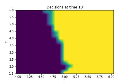 Figure 1
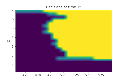 Figure 2
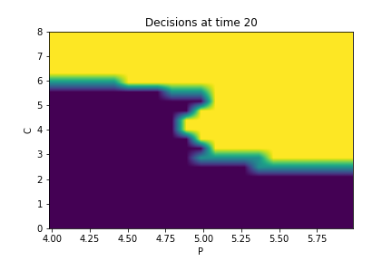 Figure 3
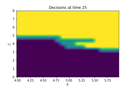 Figure 4
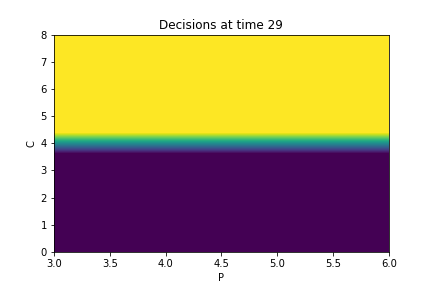 Figure 5
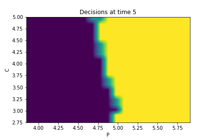 Figure 6
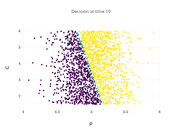 Figure 7
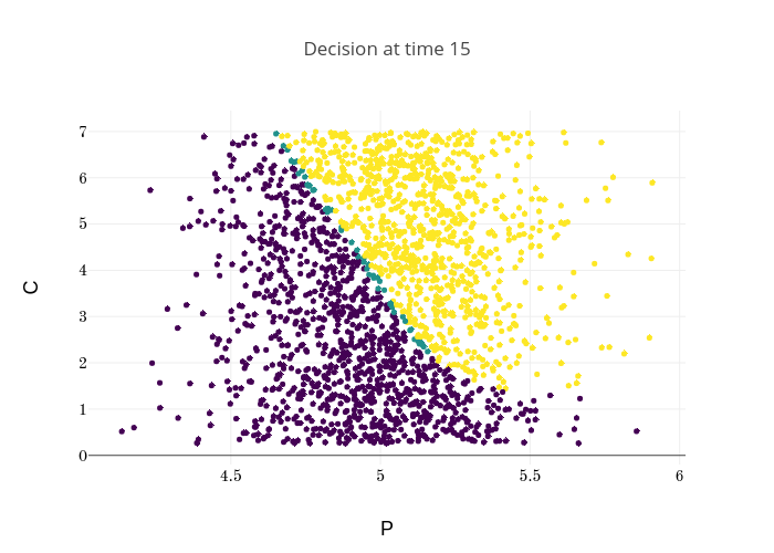 Figure 8
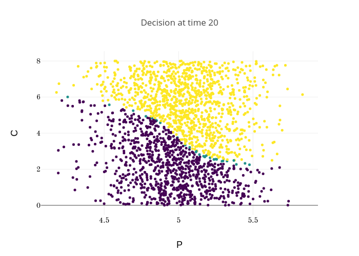 Figure 9
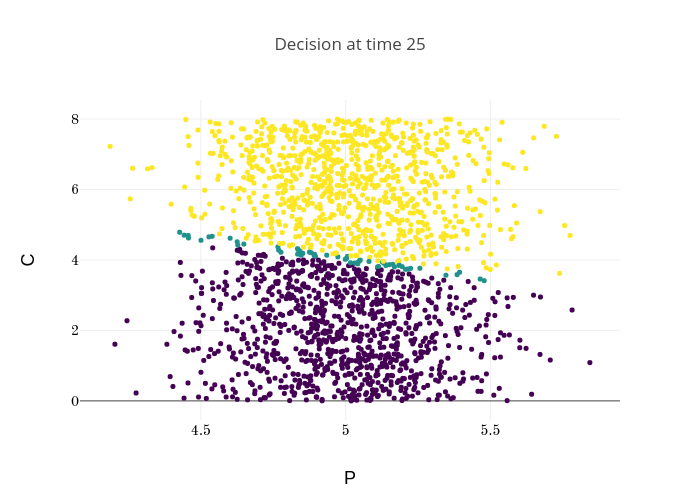 Figure 10
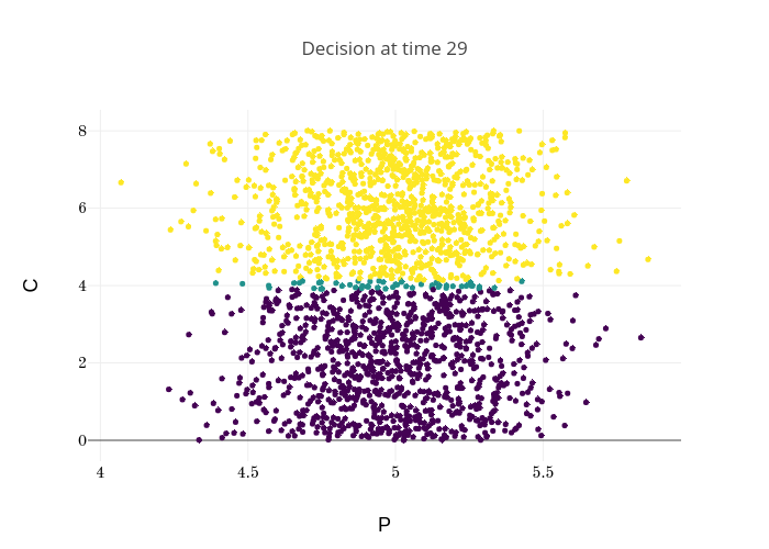 Figure 11
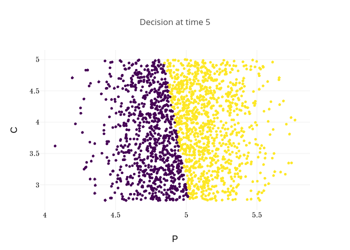 Figure 12
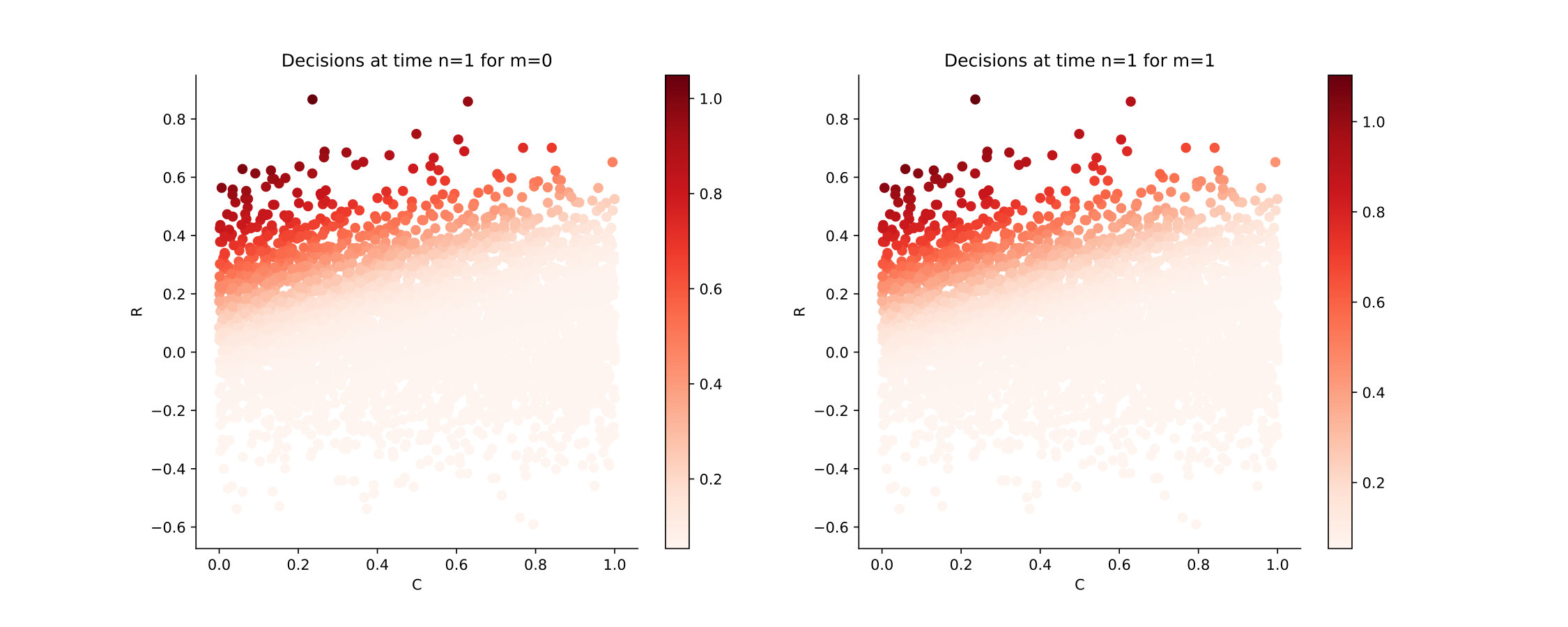 Figure 13
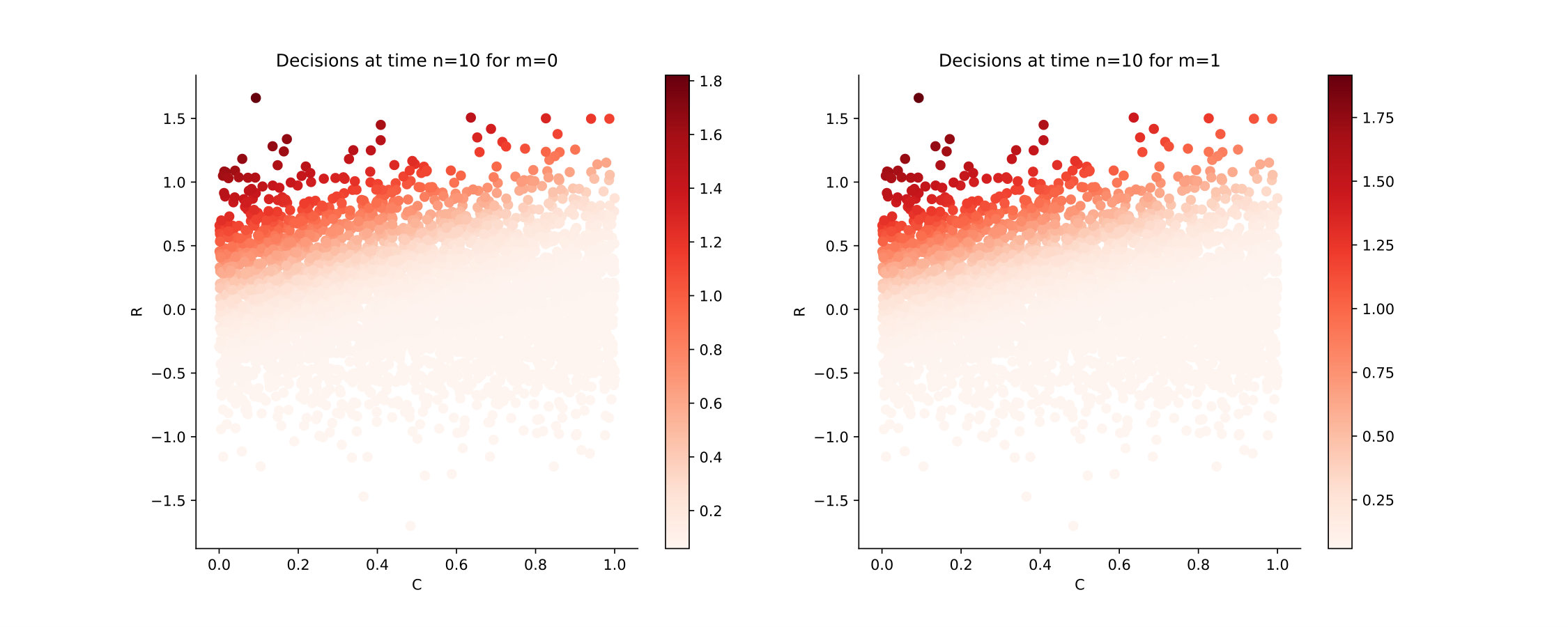 Figure 14
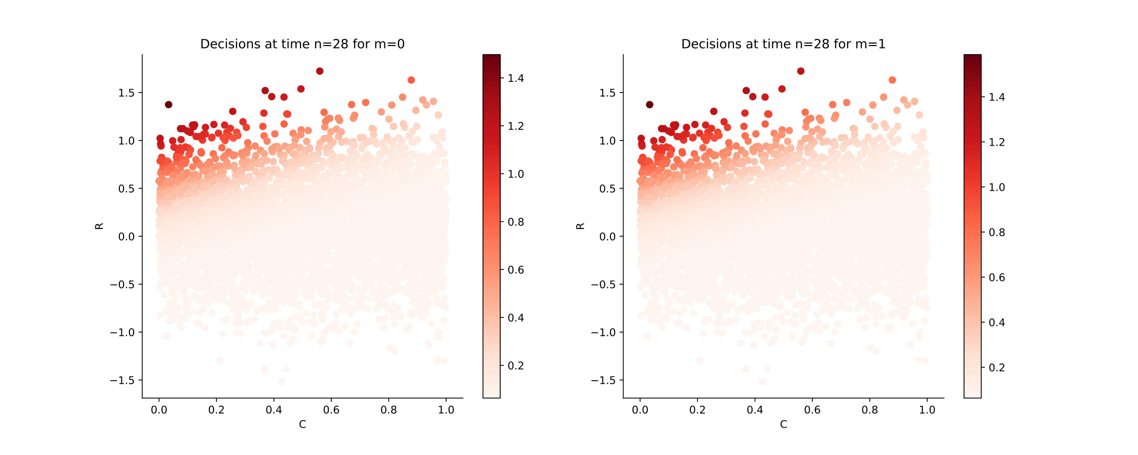 Figure 15
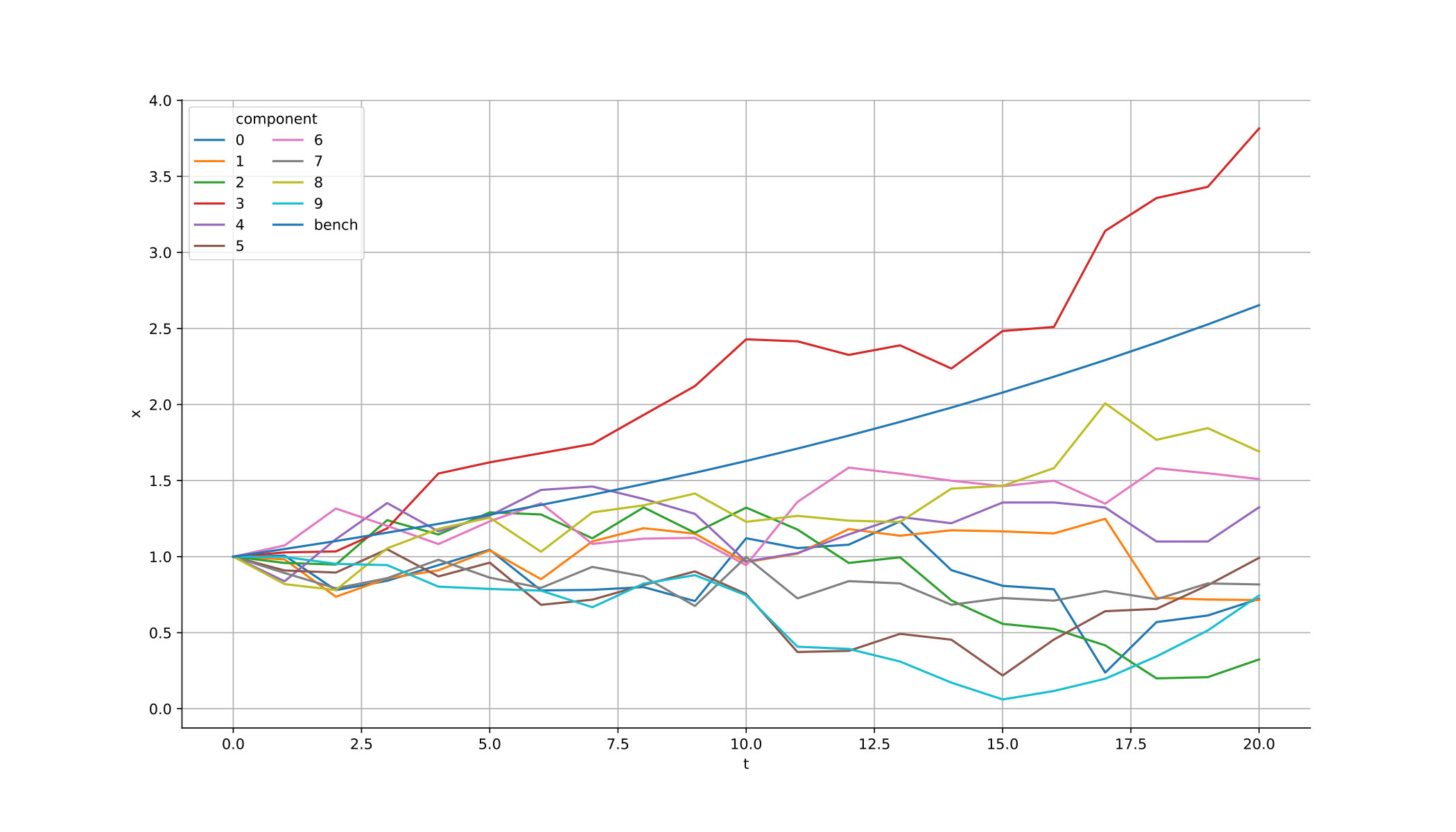 Figure 16
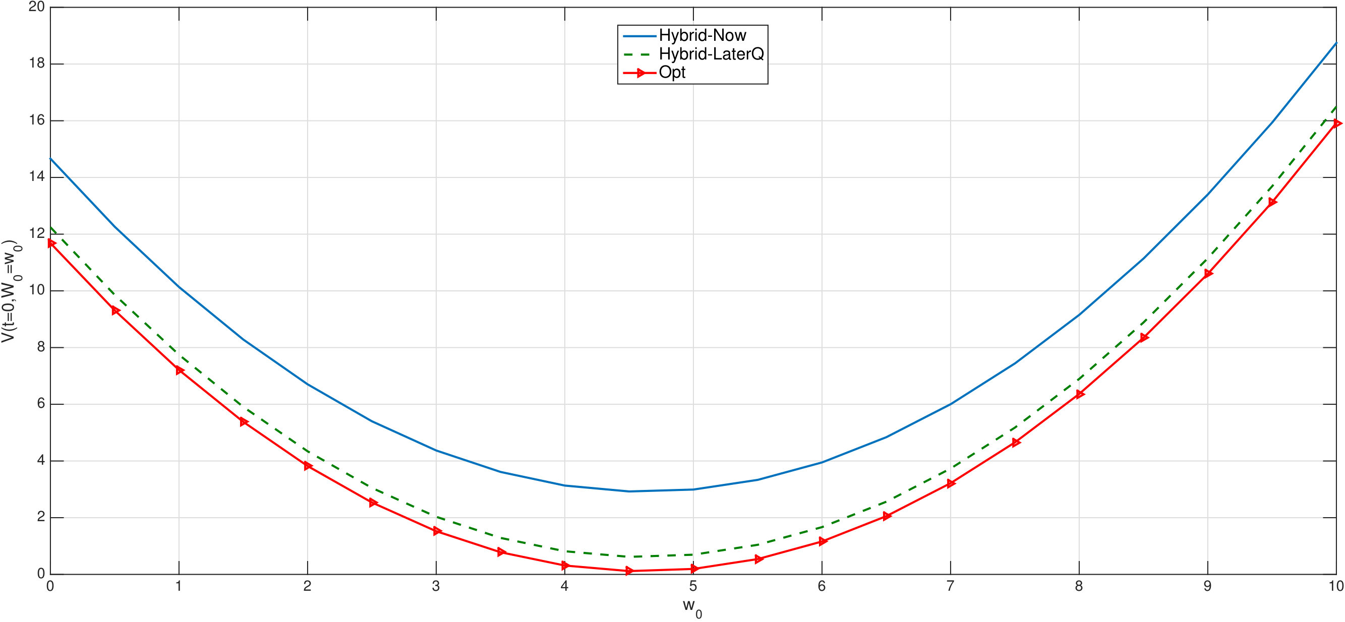 Figure 17
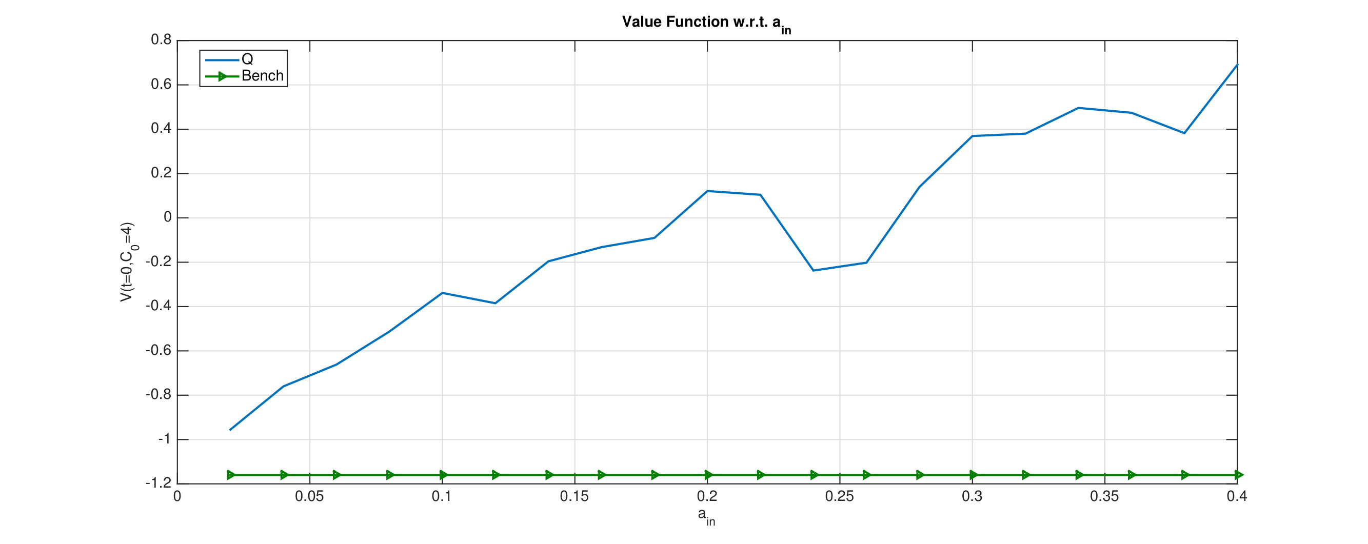 Figure 18
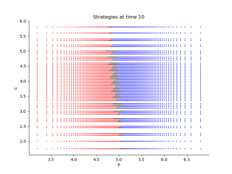 Figure 19
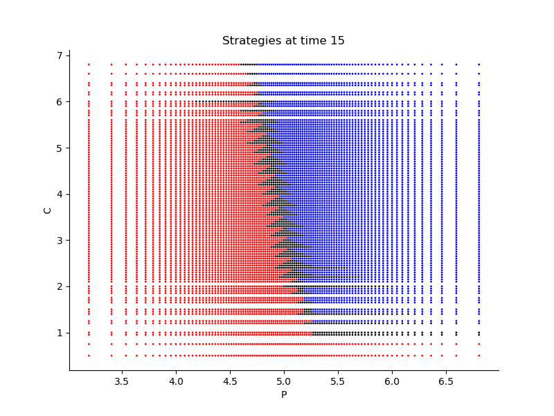 Figure 20
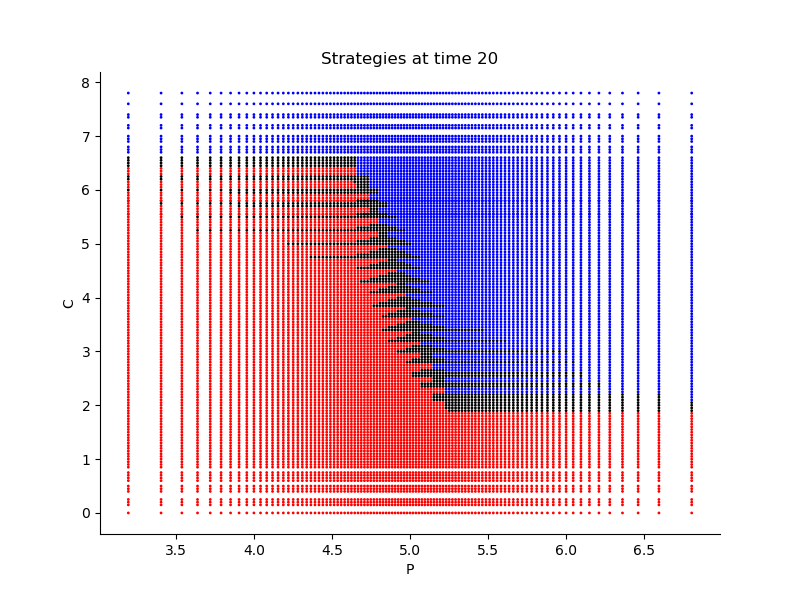 Figure 21
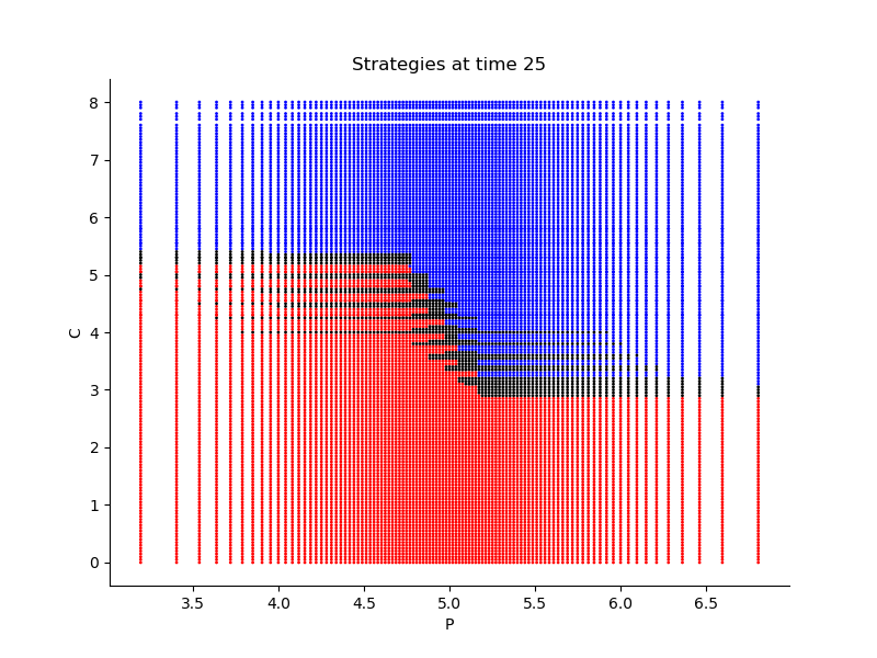 Figure 22
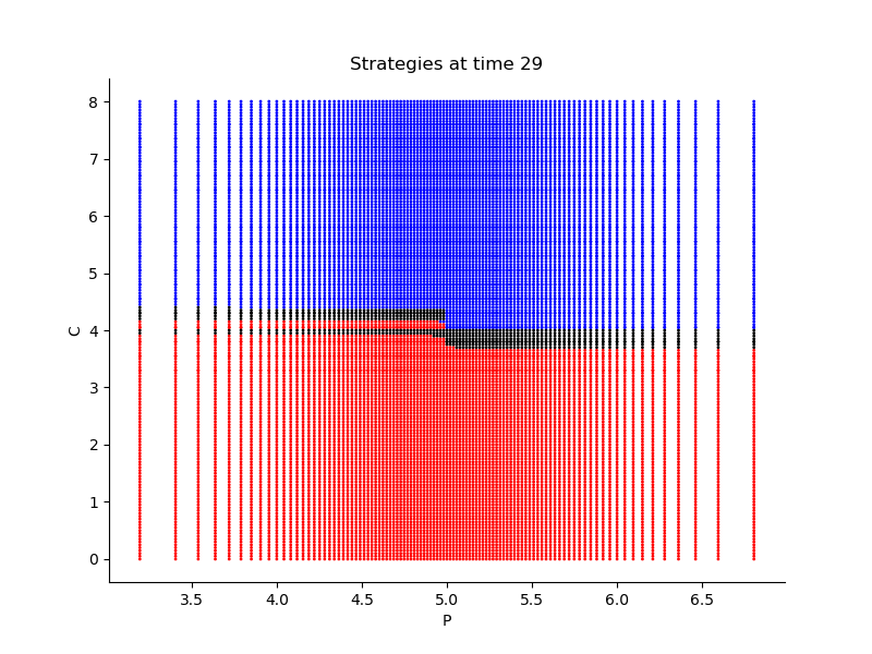 Figure 23
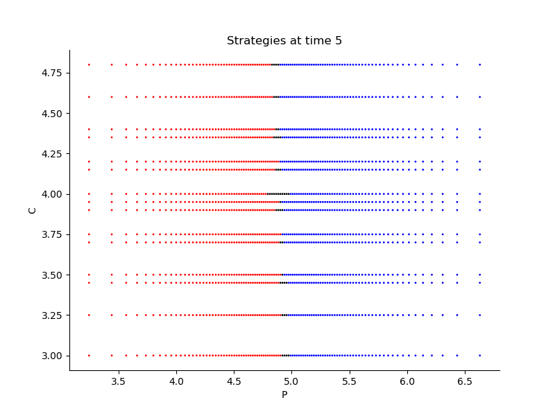 Figure 24
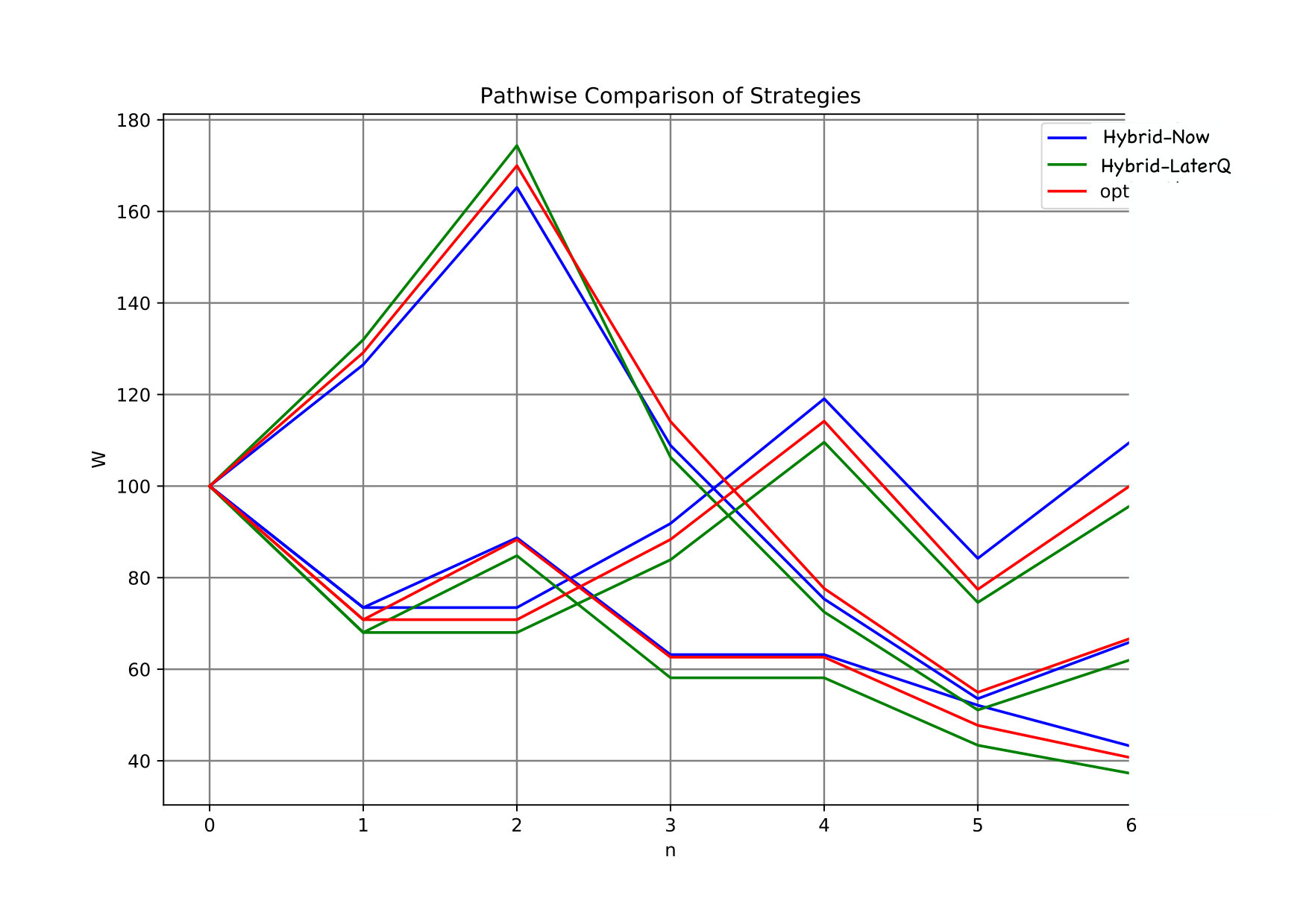 Figure 25
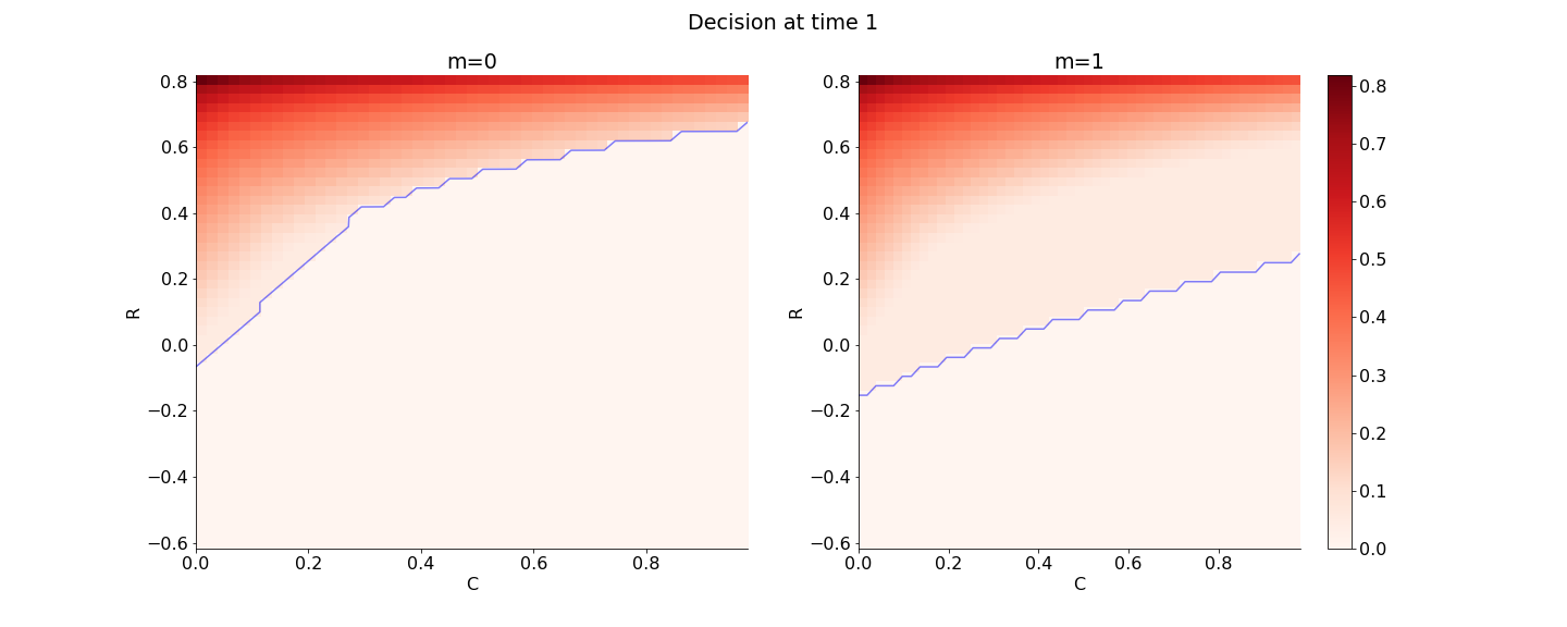 Figure 26
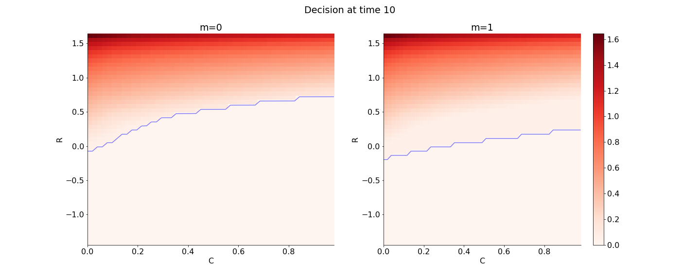 Figure 27
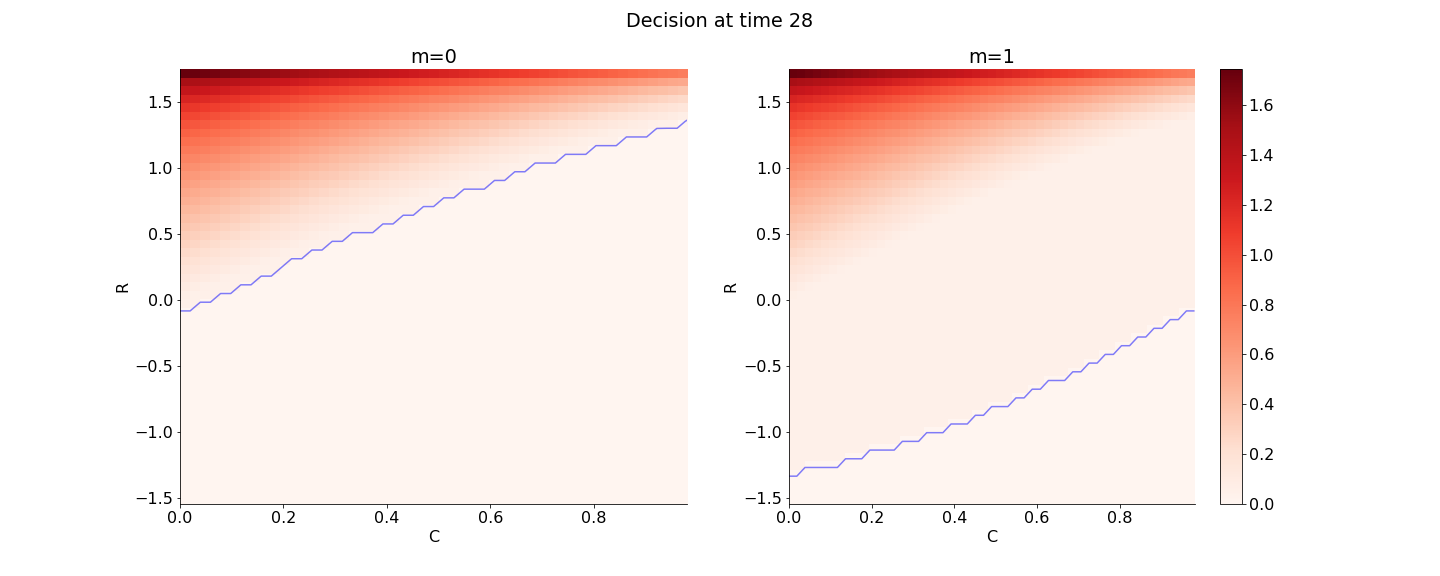 Figure 28
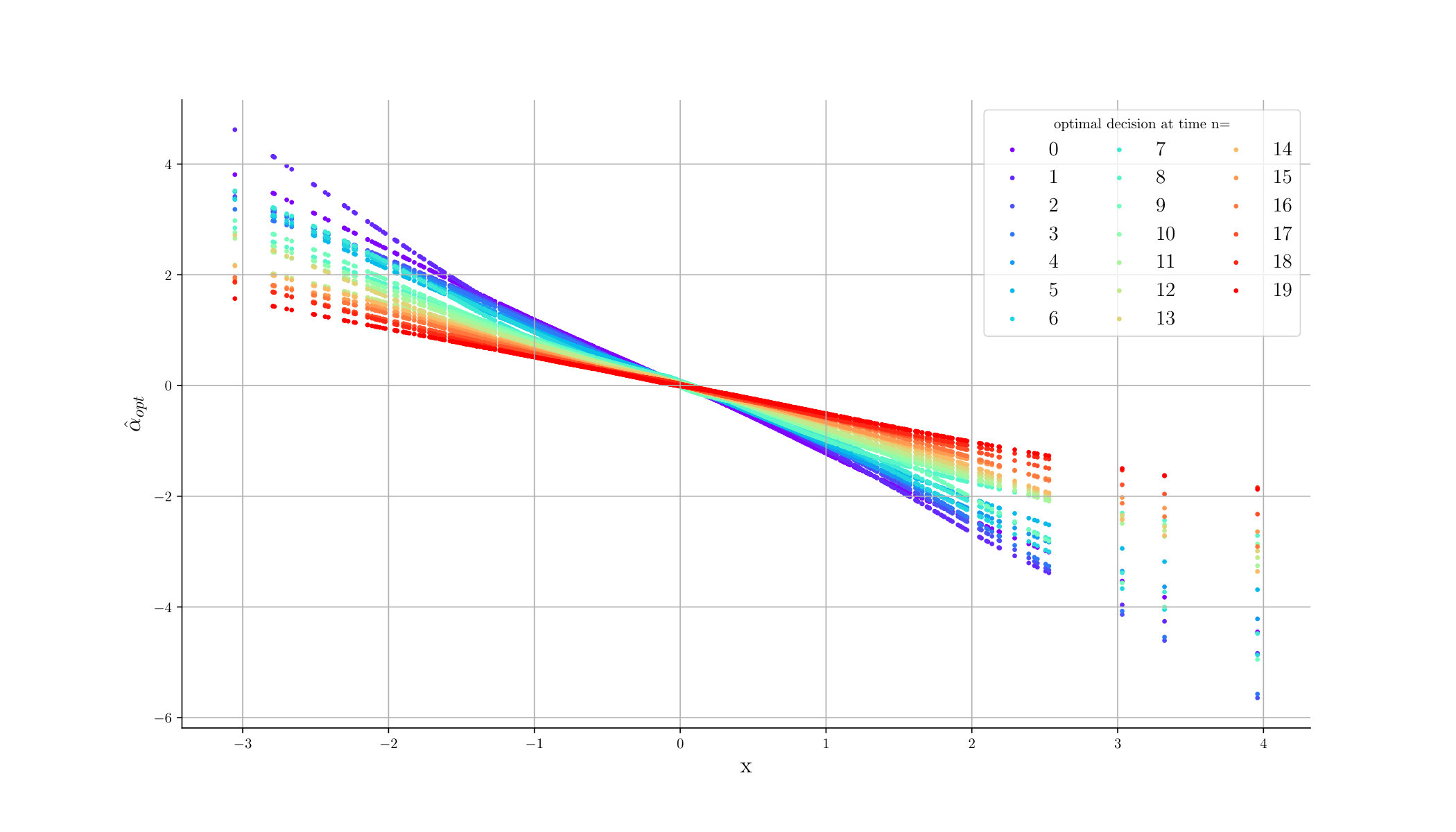 Figure 29
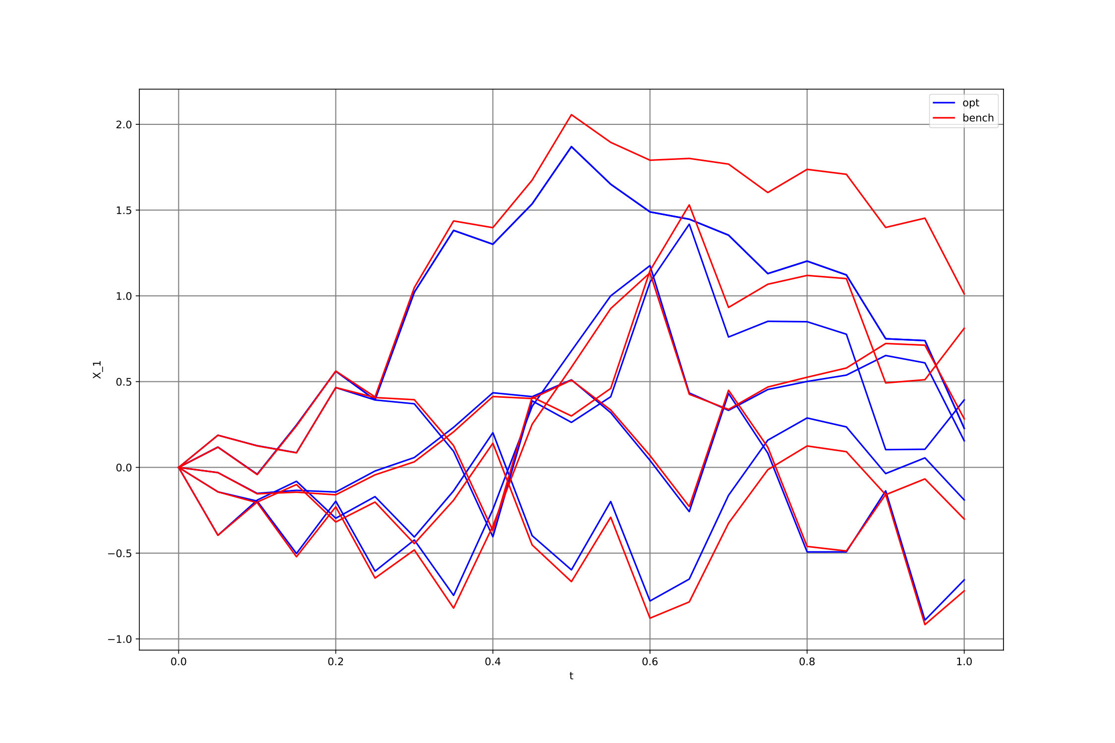 Figure 30
 Figure 31
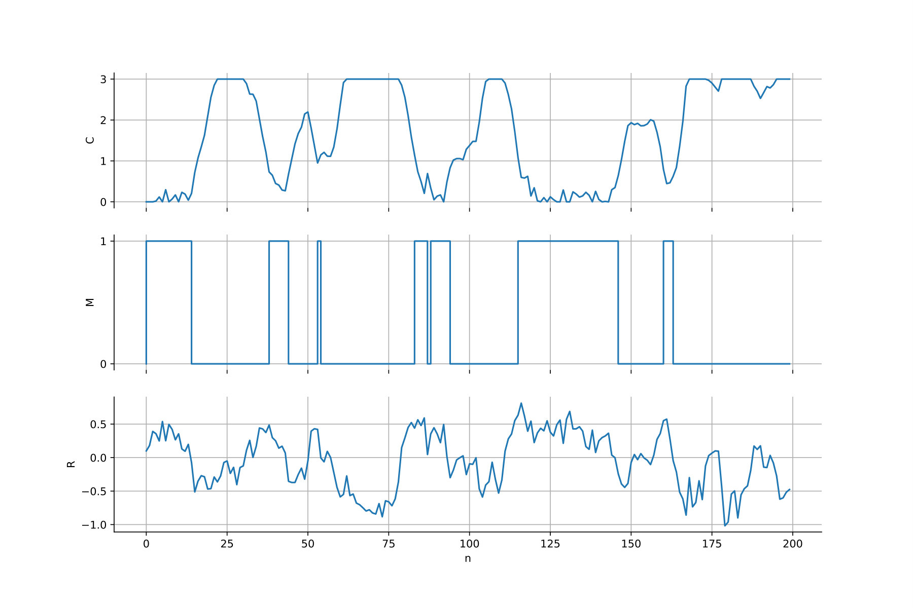 Figure 32
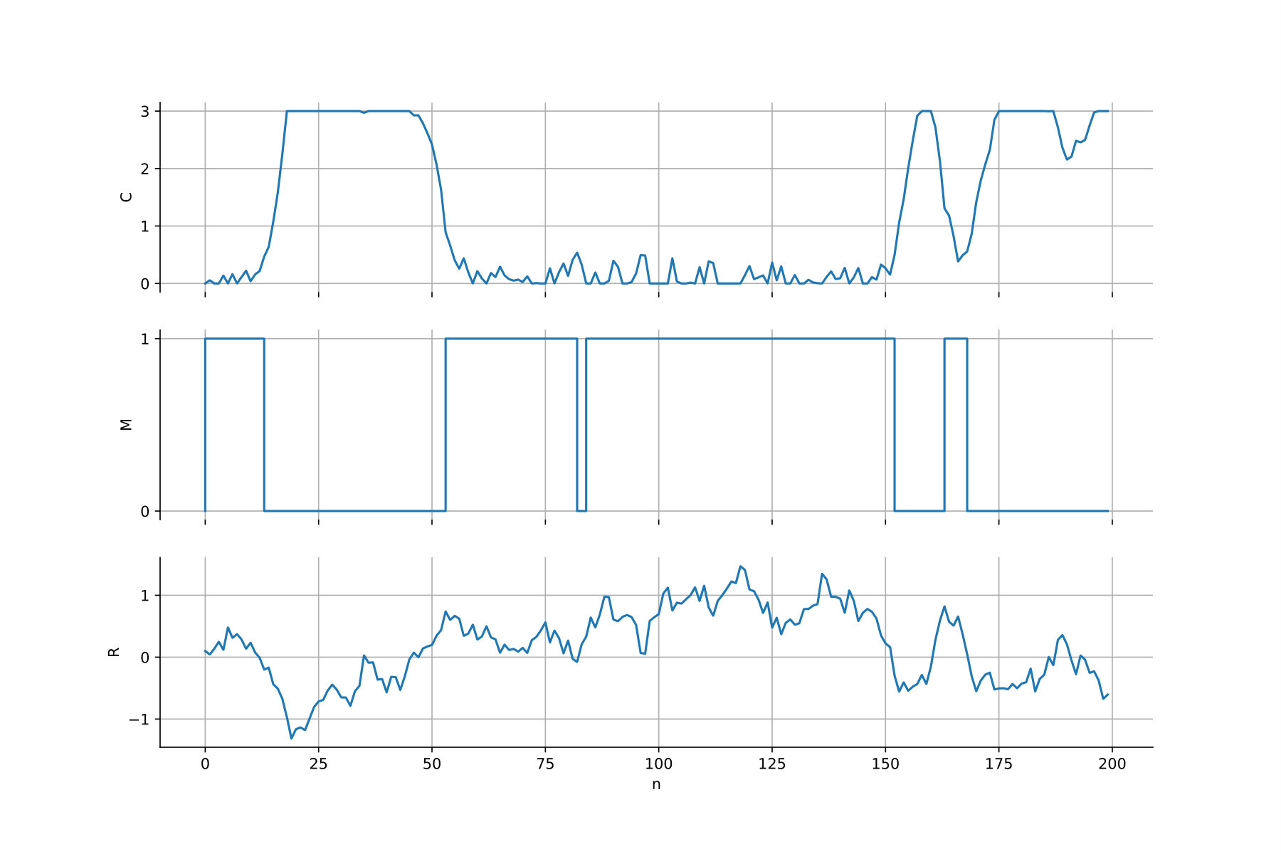 Figure 33
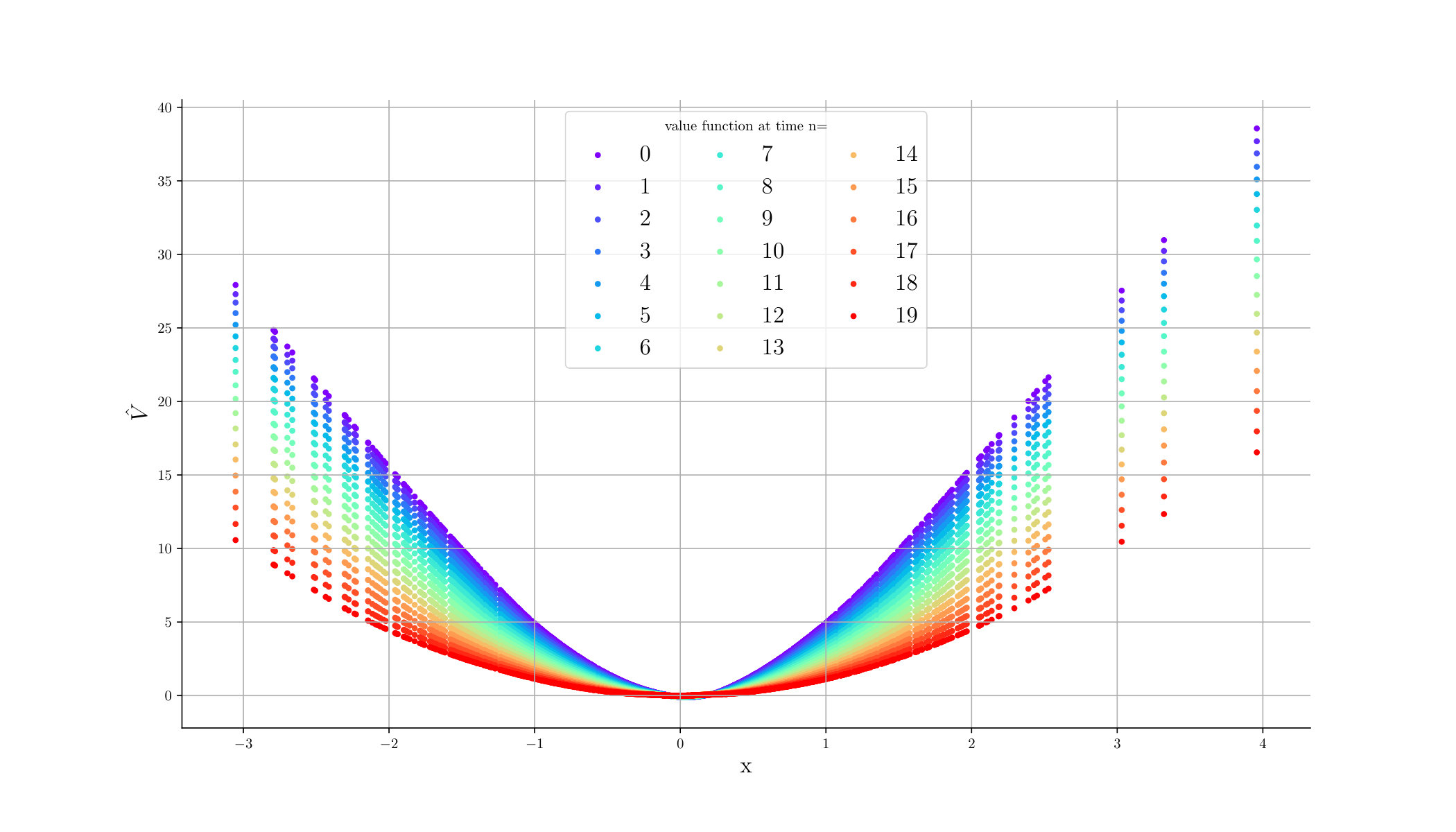 Figure 34
| Y&R | Hybrid-LaterQ | Hybrid-Now | Qknn | Bench | |
|---|---|---|---|---|---|
| 1.0 | -0.402 | -0.456 | -0.460 | -0.461 | -0.464 |
| 0.5 | -0.466 | -0.495 | -0.507 | -0.508 | -0.509 |
| 0.1 | -0.573 | -0.572 | -0.579 | -0.581 | -0.586 |
| 0.0 | -0.620 | -1.000 | -1.000 | -1.000 | -1.000 |
| Mean | std | |
|---|---|---|
| Hybrid-Now | 56.0 | 0.6 |
| NNContPI | 54.3 | 0.1 |
| Riccati | 57.1 | - |
| Mean | std | |
|---|---|---|
| Hybrid-Now | 5.7 | 7e-3 |
| NNContPI | 5.4 | 7e-3 |
| Riccati | 5.7 | - |
| Hybrid-Now | ClassifPI | Qknn | ||
|---|---|---|---|---|
| 0.06 | -0.99 | -0.71 | -0.66 | -1.20 |
| 0.10 | -0.70 | -0.38 | -0.34 | -1.20 |
| 0.20 | -0.21 | 0.01 | 0.12 | -1.20 |
| 0.30 | -0.10 | 0.37 | 0.37 | -1.20 |
| 0.40 | 0.10 | 0.51 | 0.69 | -1.20 |
| Mean | std | |
|---|---|---|
| ClassifHybrid | 33.34 | 0.31 |
| Qknn | 35.37 | 0.34 |
| Mean | Standard Deviation |
| 231.8 | 1.2 |
Peer Reviews
No public reviews on file for this paper yet. If you reviewed it on a platform where reviews are public (OpenReview, ICLR, NeurIPS, ICML), you can paste yours below so the community can read it here.
Videos
No videos yet. Explain this paper in a talk, walkthrough, or lecture? Add one.
Deep neural networks algorithms for stochastic control problems
on finite horizon: numerical applications††thanks: We are grateful to both referees for helpful comments and remarks.
Achref Bachouch aaaDepartment of Mathematics, University of Oslo, Norway. The author’s research is carried out with support of the Norwegian Research Council, within the research project Challenges in Stochastic Control, Information and Applications (STOCONINF), project number 250768/F20 achrefb at math.uio.no Côme Huré bbbLPSM, University Paris Diderot hure at lpsm.paris Nicolas Langrené cccCSIRO Data61, RiskLab Australia Nicolas.Langrene at data61.csiro.au Huyên Pham dddLPSM, University Paris-Diderot and CREST-ENSAE, pham at lspm.paris The work of this author is supported by the ANR project CAESARS (ANR-15-CE05-0024), and also by FiME and the “Finance and Sustainable Development” EDF - CACIB Chair
Abstract
This paper presents several numerical applications of deep learning-based algorithms for discrete-time stochastic control problems in finite time horizon that have been introduced in [Hur+18]. Numerical and comparative tests using TensorFlow illustrate the performance of our different algorithms, namely control learning by performance iteration (algorithms NNcontPI and ClassifPI), control learning by hybrid iteration (algorithms Hybrid-Now and Hybrid-LaterQ), on the -dimensional nonlinear PDEs examples from [EHJ17] and on quadratic backward stochastic differential equations as in [CR16]. We also performed tests on low-dimension control problems such as an option hedging problem in finance, as well as energy storage problems arising in the valuation of gas storage and in microgrid management. Numerical results and comparisons to quantization-type algorithms Qknn, as an efficient algorithm to numerically solve low-dimensional control problems, are also provided.
Keywords: Deep learning, policy learning, performance iteration, value iteration, Monte Carlo, quantization.
1 Introduction
This paper is devoted to the numerical resolution of discrete-time stochastic control problem over a finite horizon. The dynamics of the controlled state process valued in is given by
[TABLE]
where is a sequence of i.i.d. random variables valued in some Borel space , and defined on some probability space equipped with the filtration generated by the noise ( is the trivial -algebra), the control is an -adapted process valued in , and is a measurable function from into which is known by the agent. Given a running cost function defined on and a terminal cost function defined on , the cost functional associated with a control process is
[TABLE]
In this framework, we assume and to be known by the agent. The set of admissible controls is the set of control processes satisfying some integrability conditions ensuring that the cost functional is well-defined and finite. The control problem, also called Markov decision process (MDP), is formulated as
[TABLE]
and the goal is to find an optimal control , i.e., attaining the optimal value: . Notice that problem (1.1)-(1.3) may also be viewed as the time discretization of a continuous time stochastic control problem, in which case, is typically the Euler scheme for a controlled diffusion process.
It is well-known that the global dynamic optimization problem (1.3) can be reduced to local optimization problems via the dynamic programming (DP) approach, which allows to determine the value function in a backward recursion by
[TABLE]
Moreover, when the infimum is attained in the DP formula (1.4) at any time by , we get an optimal control in feedback form (policy) given by: where is the Markov process defined by
[TABLE]
The practical implementation of the DP formula may suffer from the curse of dimensionality and large complexity when the state space dimension and the control space dimension are high. In [Hur+18], we proposed algorithms relying on deep neural networks for approximating/learning the optimal policy and then eventually the value function by performance/policy iteration or hybrid iteration with Monte Carlo regressions now or later. This research led to three algorithms, namely algorithms NNcontPI, Hybrid-Now and Hybrid-LaterQ that are recalled in Section 2, and which can be seen as a natural extension of actor-critic methods, developed in the reinforcement learning community for stationary stochastic problem ([SB98]), to finite-horizon control problems. Note that for stationary control problem, it is usual to use techniques such as temporal difference learning, which relies on the fact that the value function and the optimal control do not depend on time, to improve the learning of the latter. Such techniques do not apply to finite horizon control problems. In Section 3, we perform some numerical and comparative tests to illustrate the efficiency of our different algorithms, on -dimensional nonlinear PDEs examples as in [EHJ17] and quadratic Backward Stochastic Differential equations as in [CR16], as well as on high-dimensional linear quadratic stochastic control problems. We present numerical results for an option hedging problem in finance, and energy storage problems arising in the valuation of gas storage and in microgrid management. Numerical results and comparisons to quantization-type algorithms Qknn, introduced in this paper as an efficient algorithm to numerically solve low-dimensional control problems, are also provided. Finally, we conclude in Section 4 with some comments about possible extensions and improvements of our algorithms.
2 Algorithms
We introduce in this section four neural network-based algorithms for solving the discrete-time stochastic control problem (1.1)-(1.3). The convergence of these algorithms have been analyzed in detail in our companion paper [Hur+18], and for self-contained purpose, we recall in this section the description of these algorithms and the convergence results. We also introduce at the end of this section a quantization and -nearest-neighbor-based algorithm (Qknn) that will be used as benchmark when testing our algorithms on low-dimensional control problems.
We are given a class of deep neural networks (DNN) for the control policy represented by the parametric functions , with parameters , and a class of DNN for the value function represented by the parametric functions: , with parameters . Recall that these DNN functions and are compositions of linear combinations and nonlinear activation functions, see [GBC16].
Additionally, we shall be given a sequence of probability measures on the state space , that we call training measure and denoted , which should be seen as dataset providers to learn the optimal strategies and the value functions at time .
Remark 2.1** **(Training sets design)
The choice of the training sets is critical for numerical efficiency. This problem has been largely investigated in the reinforcement learning community, notably with multi-armed bandits algorithms [ACBF02], and more recently in the numerical probability literature, see [LM19], but remains a challenging issue. Here, two cases are considered for the choice of the training measure used to generate the training sets on which the estimates at time will be computed. The first one is a knowledge-based selection, relevant when the controller knows with a certain degree of confidence where the process has to be driven in order to optimize her cost functional. The second case is when the controller has no idea where or how to drive the process to optimize the cost functional.
(1) Exploitation only strategy
In the knowledge-based setting, there is no need for exhaustive and expensive (in time mainly) exploration of the state space, and the controller can take a training measure that assigns more points in the region of the state space that is likely to be visited by the optimally-driven process.
In practice, at time , assuming we know that the optimal process is likely to lie in a region , we choose a training measure in which the density assigns a lot of weight to the points of , for example , the uniform distribution in .
(2) Explore first, exploit later When the controller has no idea where or how to drive the process to optimize the cost functional, we suggest to build the training measures as empirical measures of the process, driven by estimates of the optimal control computed using alternative methods.
- (i)
Explore first: Use an alternative method to obtain good estimates of the optimal strategy. In high-dimension: one can for example think of approximating the control at all time by neural network, and obtain a good estimate of the optimal control by performing a global optimization of the function:
[TABLE]
where is the process controlled by the feedback control at time .
- (ii)
Exploit later: Take the training measures , for , where is driven using the optimal control estimated in step (i); and apply the procedure (1). Such an idea has been recently exploited in [KPX18].
Remark 2.2** **(Choice of Neural Networks)
Unless otherwise specified, we use feed-forward Neural Networks with two or three hidden layers and +10 neurons per hidden layer, since we noticed empirically that these parameters were enough to approximate the relatively smooth objective functions considered here. We tried sigmoid, tanh, ReLU and ELU activation functions and noticed that ELU is most often the one providing the best results in our applications. We normalize the input data of each neural network in order to speed up the training of the latter. * *
Remark 2.3** **(Neural Networks Training)
We use the Adam optimizer, as implemented in TensorFlow, with initial learning-rate set to 0.001 or 0.005, which are the default values in TensorFlow, to train by gradient-descent the optimal strategy and the value function defined in the algorithms described later. TensorFlow takes care of the Adam gradient-descent procedure by automatic differentiation when the function to optimize is an expectation of TensorFlow functions, such as the usual differentiable activation functions but also popular non-differentiable activation functions such as ReLu: .
In order to force the weights and biases of the neurons to stay small, we use an regularization with parameter mainly set to 0.01, but the value can change in order to make sure that the regularization term is neither too strong or too weak when added to the loss when training neural networks.
We consider a large enough number of mini-batches of size 64 or 128 for the training, depending essentially empirically on the dimension of the problem. We use at least 10 epochseeeWe denote by epoch one pass of the full training set. and stop the training when the loss computed on a validation set of size 100 stops decreasing. We noticed that taking more than one epoch really improves the quality of the estimates. * *
Remark 2.4** **(Constraints)
The proposed algorithms can deal with state and control constraints at any time, which is useful in several applications:
[TABLE]
where is some given subset of . In this case, in order to ensure that the set of admissible controls is not empty, we assume that the sets
[TABLE]
are non empty for all , and the DP formula now reads
[TABLE]
From a computational point of view, it may be more convenient to work with unconstrained state/control variables, hence by relaxing the state/control constraint and introducing into the running cost a penalty function : , and . For example, if the constraint set is in the form: , for some functions , then one can take as penalty functions:
[TABLE]
where [math] are penalization coefficients (large in practice). * *
2.1 Control Learning by Performance Iteration
We present in this section Algorithm 1, which combines an optimal policy estimation by neural networks and the dynamic programming principle. We rely on the performance iteration procedure, i.e. paths are always recomputed up to the terminal time .
2.1.1 Algorithm NNContPI
Our first algorithm, referred to as NNContPI, is well-designed for control problems with continuous control space such as or a ball in . The main idea is:
Represent the controls at time by neural networks in which the activation function for the output layers takes values in the control space. For example, one can take the identity function as activation function for the output layer if the control space is ; or the sigmoïd function if the control space is . 2. 2.
Learn sequentially in time, and in a backward way, the optimal parameters for the representation of the optimal control. In particular, notice that the learning of the optimal control at time highly relies on the accuracy of the estimates of the optimal controls at time , computed previously.
2.1.2 Algorithm ClassifPI
In the special case where the control space is finite, i.e., Card with , a classification method can be used: consider a DNN that takes state as input and returns a probability vector with parameters . Such a usual DNN can be build using hidden layers with ReLu activation functions, an output layer with neurons, and a SoftmaxfffThe Softmax function is defined as follows: where are part of the parameters that will be learned by gradient-descent. activation function for the output layer. Algorithm 2, presented below, is based on this idea, and is called ClassifPI.
Note that, when using Algorithms 1 and 2, the estimate of the optimal strategy at time highly relies on the estimates of the optimal strategy at time , that have been computed previously. In particular, the practitioner who wants to use Algorithms 1 and 2 needs to keep track of the estimates of the optimal strategy at time in order to compute the estimate of the optimal strategy at time .
Remark 2.5
In practice, for , one should minimize the expectations (LABEL:computa) and (LABEL:computPI) by stochastic gradient-descent, where mini-batches of finite number of paths are generated by drawing independent samples under for the initial position at time , and independent samples under , for . The convergence of Algorithms 1 and 2 is analyzed in [Hur+18] in terms of the error approximation of the optimal control by neural networks, and in terms of the estimation error by stochastic gradient descent methods, see their Theorem 4.7. * *
2.2 Control and value function learning by double DNN
We present in this section two algorithms, which in contrast with Algorithms 1 or 2, only keep track of the estimates of the value function and optimal control at time in order to build an estimate of the value function and optimal control at time .
2.2.1 Regress Now (Hybrid-Now)
The Algorithm 3, refereed to as Hybrid-Now, combines optimal policy estimation by neural networks and dynamic programming principle, and relies on an hybrid procedure between value and performance iteration.
Remark 2.6
One can combine different features from Algorithms 1, 2 and 3 to solve specific problems, as it has been done for example in Section 3.5, where we designed Algorithm 6 to solve a smart grid management problem. * *
2.2.2 Regress Later and Quantization (Hybrid-LaterQ)
The Algorithm 4, called Hybrid-LaterQ, combines regress-later and quantization methods to build estimates of the value function. The main idea behind Algorithm 4 is to first interpolate the value function at time by a set of basis functions, which is in the spirit of the regress-later-based algorithms, and secondly regress the interpolation at time using quantization. The usual regress-later approach requires the ability to compute closed-form conditional expectations, which limits the stochastic dynamics and regression bases that can be considered. The use of quantization avoids this limitation and makes the regress-later algorithm more generally applicable.
Let us first recall the basic ingredients of quantization. We denote by a -quantizer of the -valued random variable (typically a Gaussian random variable), that is a discrete random variable on a grid defined by
[TABLE]
where , , are Voronoi tesselations of , i.e., Borel partitions of the Euclidian space satisfying
[TABLE]
The discrete law of is then characterized by
[TABLE]
The grid points which minimize the -quantization error lead to the so-called optimal -quantizer, and can be obtained by a stochastic gradient descent method, known as Kohonen algorithm or competitive learning vector quantization (CLVQ) algorithm, which also provides as a byproduct an estimation of the associated weights . We refer to [PPP04] for a description of the algorithm, and mention that for the normal distribution, the optimal grids and the weights of the Voronoi tesselations are precomputed on the website http://www.quantize.maths-fi.com.
Quantization is mainly used in Algorithm 4 to efficiently approximate the expectations: recalling the dynamics (1.1), the conditional expectation operator for any functional is equal to
[TABLE]
that we shall approximate analytically by quantization via:
[TABLE]
Observe that the solution to (2.6) actually provides a neural network that interpolates . Hence the Algorithm 4 contains an interpolation step, and moreover, any kind of distance in can be chosen as a loss to compute . In (2.6), we decide to take the -loss, mainly because it is the one that worked the best in our applications.
Remark 2.7** **(Quantization)
In dimension 1, we used the optimal grids and weights with points, to quantize the reduced and centered normal law ; and took 100 points to quantize the reduced and centered normal law in dimension 2, i.e. . All the grids and weights for the optimal quantization of the normal law in dimension are available in http://www.quantize.maths-fi.com for . * *
2.2.3 Some remarks on Algorithms 3 and 4
As in Remark 2.5, all the expectations written in our pseudo-codes in Algorithm 3 and 4 should be approximated by empirical mean using a finite training set. The convergence of these algorithms has been analyzed in [Hur+18] in terms of the approximation error of the optimal control and value function by neural networks, in terms of the estimation error by stochastic gradient descent methods, and in terms of the quantization error (for Algorithm 4, see their Theorems 4.14 and 4.19).
Algorithms 3 or 4 are quite efficient to use in the usual case where the value function and the optimal control at time are very close to the value function and the optimal control at time , which happens e.g. when the value function and the optimal control are approximations of the time discretization of a continuous in time value function and an optimal control. In this case, it is recommended to follow this two-step procedure:
- (i)
initialize the parameters (i.e. weights and bias) of the neural network approximations of the value function and the optimal control at time to the ones of the neural network approximations of the value function and the optimal control at time .
- (ii)
take a very small learning rate parameter, for the Adam optimizer, that guarantees the stability of the parameters’ updates from the gradient-descent based learning procedure.
Doing so, one obtains stable estimates of the value function and optimal control, which is desirable. We highlight the fact that this stability procedure is applicable here since the stochastic gradient descent method benefits from good initial guesses of the parameters to be optimized. It is an advantage compared to alternative methods proposed in the literature, such as classical polynomial regressions.
2.3 Quantization with k-nearest-neighbors (Qknn-algorithm)
Algorithm 5 presents the pseudo-code of an algorithm based on the quantization and -nearest neighbors methods, called Qknn, which will be the benchmark in all the low-dimensional control problems that will be considered in Section 3 to test NNContPI, ClassifPI, Hybrid-Now and Hybrid-Later. Also, comparisons of Algorithm 5 to other well-known algorithms on various control problems in low-dimension are performed in [Bal+19], which show in particular that Algorithm 5 works very well to solve low-dimensional control problems. Actually, in our experiments, Algorithm 5 always outperforms the other algorithms based either on regress-now or regress-later methods whenever the dimension of the problem is low enough for Algorithm 5 to be feasible.
As done in Section 2.2.2, we consider a -optimal quantizer of the noise , i.e. a discrete random variable valued in a grid of points in , and with weights . We also consider grids , of points in , which are assumed to properly cover the region of that is likely to be visited by the optimally driven process at time . These grids can be viewed as samples of well-chosen training distributions where more points are taken in the region that is likely to be visited by the optimally driven controlled process (see Remark 2.1 for details on the choice of the training measure).
Remark 2.8
The estimate of the Q-value at time given by (2.7) is not continuous w.r.t. the control variable , which might cause some stability issues when running Qknn, especially during the optimization procedure (2.8). We refer to Section 3.2.2. in [Bal+19] for a detailed presentation of an extension of Algorithm 5 where the estimates of the value function is continuous w.r.t. the control variable. * *
3 Numerical applications
In this section, we test the Neural-Networks-based algorithms presented in Section 2 on different examples. In high-dimension, we first took the same example as already considered in [EHJ17] so that we can directly compare our results to theirs, and take another example from linear quadratic control problem with explicit analytic solution that is served as reference value. In low-dimension, we compared the results of our algorithms to the ones provided by Qknn, which has been introduced in Section 2 as an excellent benchmark for low-dimensional control problems.
3.1 A semilinear PDE
We consider the following semilinear PDE with quadratic growth in the gradient:
[TABLE]
By observing that for any , - , the PDE (3.1) can be written as a Hamilton-Jacobi-Bellman equation
[TABLE]
hence associated with the stochastic control problem
[TABLE]
where is the controlled process governed by
[TABLE]
is a -dimensional Brownian motion, and the control process is valued in . The time discretization (with time step ) of the control problem (3.3) leads to the discrete-time control problem (1.1)-(1.2)-(1.3) with
[TABLE]
where is a sequence of i.i.d. random variables with law , and the cost functional
[TABLE]
On the other hand, it is known that an explicit solution to (3.1) (or equivalently (3.2)) can be obtained via a Hopf-Cole transformation (see e.g. [CR16]), and is given by
[TABLE]
We choose to run tests on two different examples that have already been considered in the literature:
Test 1
Some recent numerical results have been obtained in [EHJ17] (see Section 4.3 in [EHJ17]) when and in dimension (see Table 2 and Figure 3 in [EHJ17]). Their method is based on neural network regression to solve the BSDE representation associated with the PDE (3.1), and provide estimates of the value function at time 0 and state 0 for different values of a coefficient . We plotted the results of the Hybrid-Now algorithm in Figure 1. Hybrid-Now took one hour to achieves a relative error of 0.11%, using a 4-cores 3GHz intel Core i7 CPU. We want to highlight the fact that the algorithm presented in [EHJ17] only needed 330 seconds to provide a relative error of 0.17%. However, in our experience, it is difficult to reduce the relative error from 0.17% to 0.11% using their algorithm. Also, we believe that the computation time of our algorithm can easily be reduced; some ideas in this direction are discussed in Section 4. The main trick that can be used is the transfer learning (also referred to as pre-training in the literature): we rely on the continuity of the value function and the optimal control w.r.t. time to claim that the value function and the optimal control at time are very close to the ones at time . Hence, one can initialize the weights of the value function and optimal control at time with the optimal ones estimated at step , reduce the learning rate of the optimizer algorithm, and reduce the number of steps for the gradient descent algorithm. All this procedure really speeds up the learning of the value function and the optimal control, and insures stability of the estimates. Doing so, we were able to reduce the computation time from one hour to twenty minutes.
We also considered the same problem in dimension , for which we plotted the first component of w.r.t. time in Figure 2, for five different paths of the Brownian motion, where for each , the agent follows either the naive ( [math]) or the Hybrid-Now strategy. One can see that both strategies are very similar when the terminal time is far; but the Hybrid-Now strategy clearly forces to get closer to 0 when the terminal time gets closer, in order to reduce the terminal cost.
Let us provide further implementation details on the algorithms presented in Test 1:
- •
As one can guess from the representation of in (3.3), it is probably optimal to drive the process around 0. Hence we decided to take as a training measure at time to learn the optimal strategy and value function at time , for .
- •
We tested the algorithm with 1, 2 and 3 layers for the representation of the value function and the optimal control by neural networks, and noticed that the quality of the estimate significantly improves when using more than one layer, but does not vary significantly when considering more than 3 layers.
Test 2
Tests of the algorithms are proposed in dimension 1 with the terminal cost and . This problem was already considered in [Ric10], where the author proposed an algorithm based on a smart temporal discretization of the BSDE representation of the PDE (3.1) in order to deal with the quadratic growth of the driver of the BSDE, and usual projection on basis functions techniques for the approximation of conditional expectations that appear in the dynamic programming equation associated with the BSDE. We refer to equations (13),(14),(15) in [Ric11] for details on the proposed algorithm, and its Theorem 4.14 for the convergence result. Their estimates of the value function at time 0 and state 0, when , are available in [Ric10], and have been reported in the column of Table 1. Also, the exact values for the value function have been computed for these values of by Monte Carlo using the closed-form formula (3.4), and are reported in the column Bench of Table 1. Tests of the Hybrid-Now and Hybrid-LaterQ algorithms have been run, and the estimates of the value function at time 0 and state [math] are reported in the Hybrid-Now and Hybrid-LaterQ columns. We also tested Qknn and reported its results in column Qknn. Note that Qknn is particularly well-suited to 1-dimensional control problems. In particular, it is not time-consuming since the dimension of the state space is =1. Actually, it provides the fastest results, which is not surprising since the other algorithms need time to learn the optimal strategy and value function through gradient-descent method at each time step . Moreover, Table 1 reveals that Qknn is the most accurate algorithm on this example, probably because it uses local methods in space to estimate the conditional expectation that appears in the expression of the -value.
We end this paragraph by giving some implementation details for the different algorithms as part of Test 2:
- •
Y&R: The algorithm Y&R converged only when using a Lipschitz version of . The following approximation was used to obtain the results in Table 1:
[TABLE]
- •
Hybrid-Now: We used time steps for the time-discretization of . The value functions and optimal controls at time are estimated using neural networks with 3 hidden layers and 10+5+5 neurons.
- •
Hybrid-LaterQ: We used time steps for the time-discretization of . The value functions and optimal controls at time are estimated using neural networks with 3 hidden layers containing 10+5+5 neurons; and 51 points for the quantization of the exogenous noise.
- •
Qknn: We used time steps for the time-discretization of . We take 51 points to quantize the exogenous noise, , for ; and decided to use the 200 points of the optimal grid of for the state space discretization.
The main conclusion regarding the results in this semilinear PDE problem is that Hybrid-Now provides better estimates of the solution to the PDE in dimension =100 than the previous results available in [EHJ17] but requires more time to do so.
Hybrid-Now and Hybrid-Later provide better results than those available in [Ric11] to solve the PDE in dimension 2; but are outperformed by Qknn, which is arguably very accurate.
3.2 A linear quadratic stochastic test case
We consider a linear controlled process with dynamics in according to
[TABLE]
where , , are independent real-Brownian motion, the control process is valued in , and the constant coefficients , , . The value function of the linear quadratic stochastic control problem is
[TABLE]
where is the solution to (3.5) starting from at time , given a control process , are nonnegative symmetric matrices, and [math]. The Bellman equation associated with this stochastic control problem is a fully nonlinear equation in the form
[TABLE]
and it is well-known, see e.g. [YZ99], that an explicit solution is given by
[TABLE]
where is a nonnegative symmetric matrix, solution to the Riccati equation
[TABLE]
while an optimal feedback control is equal to
[TABLE]
We numerically solve this problem by considering a time discretization (with time step ), which leads to the discrete-time control problem with dynamics
[TABLE]
where is a sequence of i.i.d. random variables with law , and cost functional
[TABLE]
For the numerical tests, we take , , and the following parameters:
[TABLE]
where we denote .
Numerical results
We implement our algorithms in dimension , and compare our solutions with the analytic solution via the Riccati equation (3.7) solved by MatlabhhhWe solved (3.7) with the Matlab method ode45..
- •
For , we plotted the estimates of the optimal control at time in Figure 3 and the value function in Figure 4. Observe that, as expected, the estimated optimal control is linear and the estimated value function is quadratic at each time.
- •
For , we reported in Table 2 the estimates of , computed by running forward simulations of using the estimated optimal strategy. “Riccati” is computed by solving (3.7) with Matlab. We set the initial position to . We also plotted in Figure 5 a forward simulation of the components of optimally controlled. Observe that NNContPI is more accurate than Hybrid-Now. Notice that the estimates provided by the algorithms are biased, which is due to the time discretization.
- •
For , we reported in Table 3 the estimates of the value function, computed by running forward simulations of using the estimated optimal strategy. “Riccati” is computed by solving (3.7) with Matlab. We set the initial position to and . Once again, NNContPI is slightly more accurate than Hybrid-Now, and the estimates provided by the latter are biased due to the time discretization.
Implementation details: We implemented Hybrid-Now and NNContPI using training sets from the distribution for . We represented the value function and optimal control at time , using two hidden layers with d+20 and d+10 neurons, and 1 neuron for the output layers. We used Elu as activation function for the hidden layers, and identity for the output layer.
Comments on the algorithms: Hybrid-Now behaved similarly as for the SemiLinear PDE example, and we can make the same remarks. NNContPI is much slower than Hybrid-Now, because the data have to go through the neural networks that represent the optimal controls at time , in order to estimate the optimal control at time .
3.3 Option hedging
Our third example comes from a classical hedging problem in finance. We consider an investor who trades in stocks with (positive) price process , and we denote by valued in the amount held in these assets over the period . We assume for simplicity that the price of the riskless asset is constant equal to (zero interest rate). It is convenient to introduce the return process as: , , so that the self-financed wealth process of the investor with a portfolio strategy , and starting from some capital , is governed by
[TABLE]
Given an option payoff , the objective of the agent is to minimize over her portfolio strategies her expected square replication error
[TABLE]
where is a convex function on . Assuming that the returns , are i.i.d, we are in a -dimensional framework of Section 1 with with valued in , with the dynamics function
[TABLE]
the running cost function [math] and the terminal cost . We test our algorithm in the case of a square loss function, i.e. , and when there is no portfolio constraints , and compare our numerical results with the explicit solution derived in [BKL01]: denote by the distribution of , by its mean, and by assumed to be invertible; we then have
[TABLE]
where the functions [math], and are given in backward induction, starting from the terminal condition
[TABLE]
and for , by
[TABLE]
so that , where is the initial stock price. Moreover, the optimal portfolio strategy is given in feedback form by , where is the function
[TABLE]
and is the optimal wealth associated with , i.e., . Moreover, the initial capital that minimizes , and called (quadratic) hedging price is given by
[TABLE]
Test
Take , and consider one asset with returns modeled by a trinomial tree:
[TABLE]
with , , , . Take , and consider the call option with . The price of this option is defined as the initial value of the portfolio that minimizes the terminal quadratic loss of the agent when the latter follows the optimal strategy associated with the initial value of the portfolio. In this test, we want to determine the price of the call and the associated optimal strategy using different algorithms.
Remark 3.1
The option hedging problem is linear-quadratic, hence belongs to the class of problems where the agent has ansatzes on the optimal control and the value function. Indeed, we expect here the optimal control to be affine w.r.t. and the value function to be quadratic w.r.t. . For these kind of problems, the algorithms presented in Section 2 can easily be adapted so that the expressions of the estimators satisfy the ansatzes. See (3.10) and (3.11) for the option hedging problem. * *
Numerical results
In Figure 6, we plot the value function at time 0 w.r.t , the initial value of the portfolio, when the agent follows the theoretical optimal strategy (benchmark), and the optimal strategy estimated by the Hybrid-Now or Hybrid-LaterQ algorithms. We perform forward Monte Carlo using 10,000 samples to approximate the lower bound of the value function at time 0 (see [HL17] for details on how to get an approximation of the upper-bound of the value function via duality). One can observe that while all the algorithms give a call option price approximately equal to 4.5, Hybrid-LaterQ clearly provides a better strategy than Hybrid-Now to reduce the quadratic risk of the terminal loss.
We plot in Figure 7 three different paths of the value of the portfolio w.r.t the time , when the agent follows either the theoretical optimal strategy (red), or the estimated one using Hybrid-Now (blue) or Hybrid-LaterQ (green). We set for these simulations.
Comments on Hybrid-Now and Hybrid-LaterQ
The Option Hedging problem belongs to the class of linear-quadratic control problems for which we expect the optimal control to be affine w.r.t. and the value function to be quadratic w.r.t. . It is then natural to consider the following classes of controls and functions to properly approximate the optimal controls and the values functions at time =:
[TABLE]
[TABLE]
where describes the parameters (weights+bias) associated with the neural network and describes those associated with the neural network . The notation ⊺ stands for the transposition, and for the inner product. Note that there are 2 (resp. 3) neurons in the output layer of (resp. ), so that the inner product is well-defined in (3.11) and (3.10).
3.4 Valuation of energy storage
We present a discrete-time version of the energy storage valuation problem studied in [CL10]. We consider a commodity (gas) that has to be stored in a cave, e.g. salt domes or aquifers. The manager of such a cave aims to maximize the real options value by optimizing over a finite horizon the dynamic decisions to inject or withdraw gas as time and market conditions evolve. We denote by the gas price, which is an exogenous real-valued Markov process modeled by the following mean-reverting process:
[TABLE]
where , and [math] is the stationary value of the gas price. The current inventory in the gas storage is denoted by and depends on the manager’s decisions represented by a control process valued in : (resp. ) means that she injects (resp. withdraws) gas with an injection (resp. withdrawal) rate (resp. ) requiring (causing) a purchase (resp. sale) of (resp. ), and [math] means that she is doing nothing. The difference between and (resp. and ) indicates gas loss during injection/withdrawal. The evolution of the inventory is then governed by
[TABLE]
where we set
[TABLE]
and we have the physical inventory constraint:
[TABLE]
The running gain of the manager at time is given by
[TABLE]
and represents the storage cost in each regime . The problem of the manager is then to maximize over the expected total profit
[TABLE]
where a common choice for the terminal condition is
[TABLE]
which penalizes for having less gas than originally, and makes this penalty proportional to the current price of gas ( [math]). We are then in the -dimensional framework of Section 1 with , and the set of admissible controls in the dynamic programming loop is given by:
[TABLE]
Test
We fixed the parameters as follows, to run our numerical tests:
[TABLE]
, [math], , , , with , and in the terminal penalty function, =$$30.
Numerical results
We plotted in Figure 8 the estimates of the value function at time 0 w.r.t. using Qknn, as well as the reward function (3.16) associated with the naive do-nothing strategy [math] (see Bench in figure 8). As expected, the naive strategy performs well when is small compared to , since, in this case, it takes time to fill the cave, so that the agent is likely to do nothing in order to avoid any penalization at terminal time. When is of the same order as , it is easy to fill up and empty the cave, so the agent has more freedom to buy and sell gas in the market without worrying about the terminal cost. Observe that the value function is not monotone, due to the fact that the component in the state space takes its value in a bounded and discrete set (see (3.13)).
Table 4 provides the estimates of the value function using the ClassifPI, Hybrid-Now and Qknn algorithms. Observe first that the estimates provided by Qknn are larger than those provided by the other algorithms, meaning that Qknn outperforms the other algorithms. The second best algorithm is ClassifPI, while Hybrid-Now performs poorly and clearly suffers from instability, due to the discontinuity of the running rewards w.r.t. the control variable.
Finally, Figures 9, 10, 11 provide the optimal decisions w.r.t. at times 5, 10, 15, 20, 25, 29 estimated respectively by the Qknn, ClassifPI and Hybrid-Now algorithms.
As expected, one can observe on each plot that the optimal strategy is to inject gas when the price is low, to sell gas when the price is high, and to make sure to have a volume of gas greater than in the cave when the terminal time is getting closer to minimize the terminal cost.
Let us now comment on the implementation of the algorithms:
- •
*Qknn: * Table 4 shows that once again, due to the low-dimensionality of the problem, Qknn provides the best value function estimates. The estimated optimal strategies, shown on Figure 9, are very good estimates of the theoretical ones. The three decision regions on Figure 9 are natural and easy to interpret: basically it is optimal to sell when the price is high, and to buy when it is low. However, a closer look reveals that the waiting region (where it is optimal to do nothing) has an unusual triangular-based shape, due essentially to the discreteness of the space on which the component of the state space takes its values. We expect this shape to be very hard to reproduce with the DNN-based algorithms proposed in Section 2.
- •
ClassifPI: As shown on Figure 10, the ClassifPI algorithm manages to provide accurate estimates for the optimal controls at time . However, the latter is not able to catch the particular triangular-based shape of the waiting region, which explains why Qknn performs better.
- •
Hybrid-Now: As shown on Figure 11, Hybrid-Now only manages to provide relatively poor estimates, compared to ClassifPI and Qknn, of the three different regions at time . In particular, the regions suffer from instability.
We end this paragraph by providing some implementation details for the different algorithms we tested.
- •
Qknn: We used the extension of Algorithm 5 introduced in the paragraph “semi-linear interpolation” of the Section 3.2.2. in [Bal+19] and used a projection of each state on its =2-nearest neighbors to get an estimate of the value function which is continuous w.r.t. the control variable at each time . The optimal control is computed at each point of the grids using the Brent algorithm, which is a deterministic function optimizer already implemented in PythoniiiWe could have chosen other algorithms to optimize the -value, but, in our tests, Brent was faster than the other choices that we tried, such as GoldenSearch, and always provided accurate estimates of the optimal controls..
- •
Implementation details for the neural network-based algorithms: We use neural networks with two hidden layers, ELU activation functionsjjjThe Exponential Linear Unit (ELU) activation function is defined as x\mapsto\left\{\begin{array}[]{ll}\exp(x)-1&\text{ if }x\leq 0\\ x&\text{ if }x>0\end{array}\right.. and neurons . The output layer contains 3 neurons with softmax activation function for the ClassifPI algorithm and no activation function for the Hybrid-Now one. We use a training set of size M=60,000 at each time step. Note that given the expression of the terminal cost, the ReLU activation functions (Rectified Linear Units) could have been deemed a better choice to capture the shape of the value functions, but our tests revealed that ELU activation functions provide better results. At time , we took as training measure.
We did not use the pre-train trick discussed in Section 2.2.3, which explains the instability in the decisions that can be observed in Figure 11.
The main conclusion of our numerical comparisons on this energy storage example is that ClassifPI, the DNN-based classification algorithm designed for stochastic control problems with discrete control space, appears to be more accurate than the more general Hybrid-Now. Nevertheless, ClassifPI was not able to capture the unusual triangle-based shape of the optimal control as well as Qknn did.
3.5 Microgrid management
Finally, we consider a discrete-time model for power microgrid inspired by the continuous-time models developed in [Hey+18] and [JP15]; see also [Ala+19]. The microgrid consists of a photovoltaic (PV) power plant, a diesel generator and a battery energy storage system (BES), hence using a mix of fuel and renewable energy sources. These generation units are decentralized, i.e., installed at a rather small scale (a few kW power), and physically close to electricity consumers. The PV produces electricity from solar panels with a generation pattern depending on the weather conditions. The diesel generator has two modes: on and off. Turning it on consumes fuel, and produces an amount of power . The BES can store energy for later use but has limited capacity and power. The aim of the microgrid management is to find the optimal planning that meets the power demand, denoted by , while minimizing the operational costs due to the diesel generator. We denote by
[TABLE]
the residual demand of power: when [math], one should provide power through diesel or battery, and when [math], one can store the surplus power in the battery.
The optimal control problem over a fixed horizon is formulated as follows. At any time , the microgrid manager decides the power production of the diesel generator, either by turning it off: [math], or by turning it on, hence generating a power valued in with [math] . There is a fixed cost [math] associated with switching from the on/off mode to the other one off/on, and we denote by the mode valued in of the generator right before time , i.e., .
When the diesel generator and renewable provide a surplus of power, the excess can be stored into the battery (up to its limited capacity) for later use, and in case of power insufficiency, the battery is discharged for satisfying the power demand. The input power process for charging the battery is then given by
[TABLE]
where is the maximum capacity of the battery with current charge , while the output power process for discharging the battery is given by
[TABLE]
Here, we denote . Assuming for simplicity that the battery is fully efficient, the capacity charge of the BES, valued in , evolves according to the dynamics
[TABLE]
The imbalance process defined by
[TABLE]
represents how well we are doing for satisfying electricity supply: the ideal situation occurs when [math], i.e., perfect balance between demand and generation. When [math], this means that demand is not satisfied, i.e., there is missing power in the microgrid, and when [math], there is an excess of electricity. In order to ensure that there is no missing power, we impose the following constraint on the admissible control:
[TABLE]
but penalize the excess of electricity when [math] with a proportional cost [math]. We model the residual demand as a mean-reverting process:
[TABLE]
where are i.i.d., , and . The goal of the microgrid manager is to find the optimal (admissible) decision that minimizes the functional cost
[TABLE]
where is the cost function for fuel consumption: [math], and e.g. , with [math], [math]. This stochastic control problem fits into the -dimensional framework of Section 1 (see also Remark 2.4) with control valued in , , noise , starting from an initial value on the state space , with dynamics function
[TABLE]
for , , , running cost function
[TABLE]
zero terminal cost [math], and control constraint
[TABLE]
Remark 3.2
The state/space constraint is managed in our NN-based algorithm by introducing a penalty function into the running cost (see Remark 2.4):
[TABLE]
with large taken much larger than . Doing so, the NN-based estimate of the optimal control learns not to take any forbidden decision. * *
The control space is a mix between a discrete space and a continuous space, which is challenging for algorithms with neural networks. We actually use a mixture of classification and standard DNN for the control: valued in , where is the probability of turning off in state , and is the amount of power when turning on with probability . In other words,
[TABLE]
The pseudo-code of this approach, specifically designed for this problem, is written in Algorithm 6, and we henceforth refer to it as ClassifHybrid. Note in particular that it is an Hybrid version of ClassifPI.
Test
We set the parameters to the following values to compare Qknn and ClassifHybrid:
[TABLE]
Results
Figure 12 shows the Qknn-estimated optimal decisions to take at times in the cases where [math] and . If the generator is off at time , i.e. [math], the blue curve separates the region where it is optimal to keep it off and the one where it is optimal to generate power. If the generator is on at time , i.e. , the blue curve separates the region where it is optimal to turn it off and the one where it is optimal to generate power. A colorscale is available on the right to inform how much power it is optimal to generate in both cases. Observe that the optimal decisions are quite intuitive: for example, if the demand is high and the battery is empty, then it is optimal to generate a lot of energy. Moreover, it is optimal to turn the generator off if the demand is negative or if the battery is charged enough to meet the demand.
We plot in Figure 13 the estimated optimal decisions at times , using the Hybrid-Now algorithm, with time steps. See that the decisions are similar to the ones given using Qknn.
Note that the plots in Figure 12 and 13 look much better than the ones obtained in [Ala+19] in which algorithms based on regress-now or regress-later are used (see in particular Figure 4 in [Ala+19]); hence Qknn and ClassifHybrid seem more stable than the algorithms proposed in [Ala+19].
We report in Table 5 the result for the estimates of the value function with =30 time steps, obtained by running 10 times a forward Monte Carlo with 10,000 simulations using the optimal strategy estimated using Qknn and ClassifHybrid algorithms. Observe that Hybrid-Now performs better than Qknn. However, Qknn run in less than a minute whereas Hybrid-Now needed seven minutes to run.
We also report in Table 6 the value function estimates with =200 time steps, obtained by running 20 times a forward Monte Carlo with 10,000 simulations using the Qknn-estimated optimal strategy.
Figure 14 shows two simulations of controlled using the Qknn-estimated optimal strategy, where has been chosen. Observe in particular the natural behavior of the Qknn-decisions which consists in turning the generator on when the demand cannot be met by the battery, and turn it off when the demand is negative or when the battery is charged enough to meet the demand. Note that the plots are similar to the ones plotted in Figure 9 of [Ala+19].
Comments on Qknn: Note that there is no need to use a penalization method with the Qknn-algorithm to constrain the control to stay in , where is the state at time , since, for all state , we can simply search for the optimal control associated in , using e.g. the Brent algorithm. For , we took the training set as follows: ; where , and where is the optimal grid for the quantization of , available in http://www.quantize.maths-fi.com, with 51 points. This choice of training points for the component corresponds to the exploration procedure discussed in Remark 2.1, whereas we chose the best grid with 51 points for the (uncontrolled) component.
Comments on ClassifHybrid: We took 100 mini-batches of size 300 and took 100 epochs to run the algorithm. We chose the following training distribution at time : , where is the law of the (uncontrolled) residual demand at time . Note that such a choice of training distribution means that we want to explore all the available states for the controlled components of the controlled process in order to learn the optimal strategy globally.
The microgrid management problem is very challenging for our algorithms because the control space is a mix of discrete and continuous space, moreover the choice of the optimal control is subject to constraints. We designed ClassifHybrid, an Hybrid version of ClassifPI, to solve this problem. ClassifHybrid provided very good estimates and actually managed to perform better than Qknn.
4 Discussion and conclusion
Our proposed algorithms are well-designed and provide accurate estimates of optimal control and value function associated with various high-dimensional control problems. Also, when tested on low-dimensional problems, they performed as well as the Monte Carlo-based or quantization-based methods, which have shown their efficiency in low dimension, see e.g. [Bal+19] and [Ala+19].
The presented algorithms suffer from a rather high time-consuming cost due to the expensive training of neural networks to learn the value functions and optimal controls at times . However, the agent can easily alleviate the computation time. A first trick consists in reducing the number of neural networks by partially or totally ignoring the dynamic programming principle (DPP), as it has been done e.g. in [EHJ17]. The use of one unique Recurrent Neural Networks (RNN) (in the case where the DPP is totally ignored) or a few of them (in the partial-ignored case) can also be considered to learn the optimal controls, either all at the same time (first case), or group by group in a backward way (second case). We refer to [WNMW19] for algorithms in this spirit. Another trick consists in learning faster the value functions and optimal controls at times by pre-training the neural networks. The way to proceed in that direction is to initialize at time the weights and bias of the value function estimator to the ones of . We then rely on the continuity of the value function w.r.t. the time to expect that the weights will not change much from time to , hence trainable very quickly by reducing the learning rate of the Adam algorithm for the gradient descent, and using an early-stop procedure as implemented in KeraskkkSee EarlyStopping callback in Keras. Another benefit from the pre-training task is to get the stability of the estimates w.r.t. time, which is also a pleasant feature.
The reference list from the paper itself. Each links out to its DOI / PubMed record.
- 1[ACBF 02] Peter Auer, Nicolò Cesa-Bianchi and Paul Fischer “Finite-time Analysis of the Multiarmed Bandit Problem” In Machine Learning 47.2 , 2002, pp. 235–256 DOI: 10.1023/A:1013689704352 · doi ↗
- 2[Ala+19] Clemence Alasseur, Alessandro Balata, Sahar Ben Aziza, Aditya Maheshwari, Peter Tankov and Xavier Warin “Regression Monte Carlo for Microgrid Management” In ESAIM Proceedings and Surveys, CEMRACS 2017 , 2019, pp. 46–67
- 3[Bal+19] Alessandro Balata, Côme Huré, Mathieu Laurière, Huyên Pham and Isaque Pimentel “A Class of Finite-Dimensional Numerically Solvable Mc Kean-Vlasov Control Problems” In ESAIM Proceedings and Surveys, CEMRACS 2017 19 , 2019, pp. 114–144
- 4[BKL 01] Dimitris Bertsimas, Leonid Kogan and Andrew W. Lo “Hedging derivative securities and incomplete markets: an ε 𝜀 \varepsilon -arbitrage approach” In Operations Research 49.3 , 2001, pp. 372–397
- 5[CL 10] René Carmona and Mike Ludkovski “Valuation of energy storage: an optimal switching approach” In Quantitative Finance 26.1 , 2010, pp. 262–304
- 6[CR 16] Jean-Francois Chassagneux and Adrien Richou “Numerical Simulation of Quadratic BSD Es” In The Annals of Applied Probabilities 26.1 , 2016, pp. 262–304
- 7[EHJ 17] Weinan E, Jiequn Han and Arnulf Jentzen “Deep learning-based numerical methods for high-dimensional parabolic partial differential equations and backward stochastic differential equations” In Communications in Mathematics and Statistics 5 5 , 2017, pp. 349–380
- 8[GBC 16] Ian Goodfellow, Yoshua Bengio and Aaron Courville “Deep learning” MIT Press, 2016