Kinetic modeling of the electromagnetic precursor from an axisymmetric binary pulsar coalescence
Benjamin Crinquand, Beno\^it Cerutti, Guillaume Dubus

TL;DR
This study uses kinetic simulations to explore electromagnetic precursor emissions from merging binary pulsars, revealing magnetic reconnection and high-energy radiation processes that could produce observable fast radio bursts.
Contribution
It provides the first detailed kinetic modeling of pulsar magnetosphere interactions during mergers, highlighting magnetic dissipation and particle acceleration mechanisms.
Findings
Magnetic dissipation increases as pulsars approach merger.
Magnetic reconnection drives particle acceleration and synchrotron emission.
Potential radio signals could be linked to fast radio bursts.
Abstract
The recent detection of gravitational waves associated with a binary neutron star merger revives interest in interacting pulsar magnetospheres. Current models predict that a significant amount of magnetic energy should be released prior to the merger, leading to electromagnetic precursor emission. In this paper, we revisit this problem in the light of the recent progress in kinetic modeling of pulsar magnetospheres. We limit our work to the case of aligned magnetic moments and rotation axes, and thus neglect the orbital motion. We perform global two-dimensional axisymmetric particle-in-cell simulations of two pulsar magnetospheres merging at a rate consistent with the emission of gravitational waves. Both symmetric and asymmetric systems are investigated. Simulations show a significant enhancement of magnetic dissipation within the magnetospheres as both stars get closer. Even though…
Click any figure to enlarge with its caption.
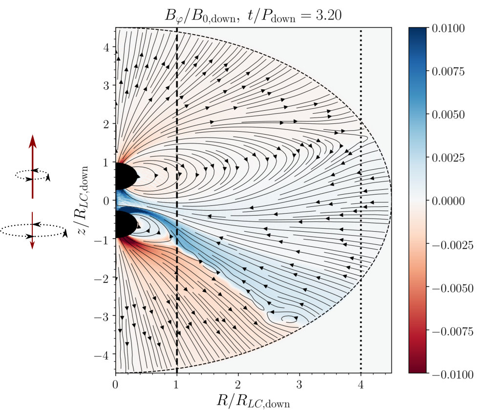 Figure 1
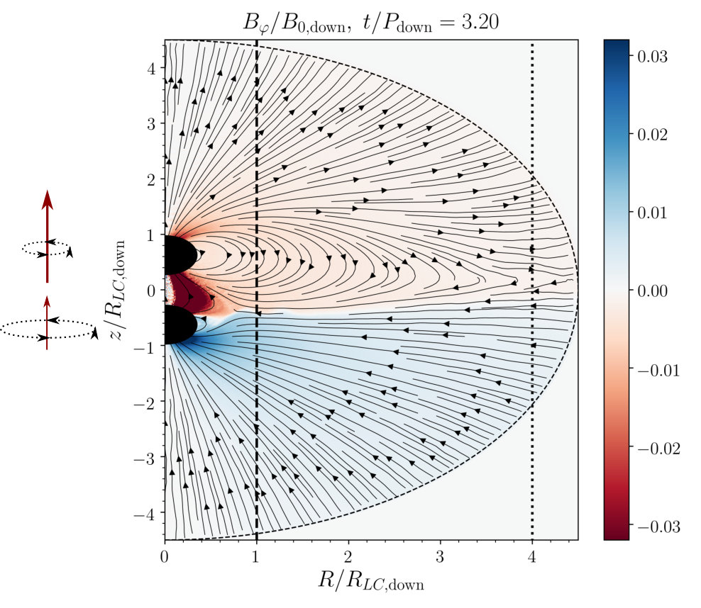 Figure 2
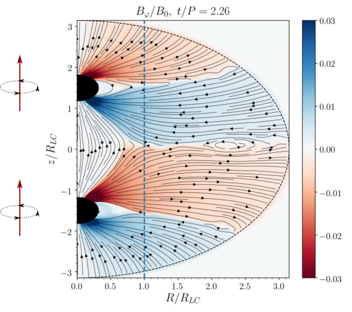 Figure 3
 Figure 4
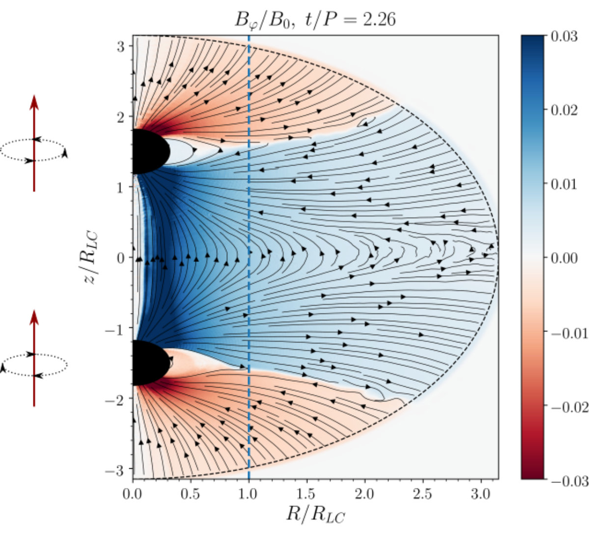 Figure 5
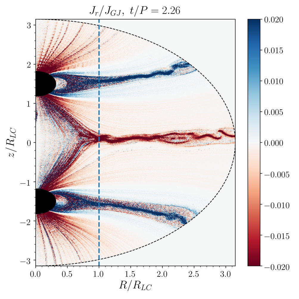 Figure 6
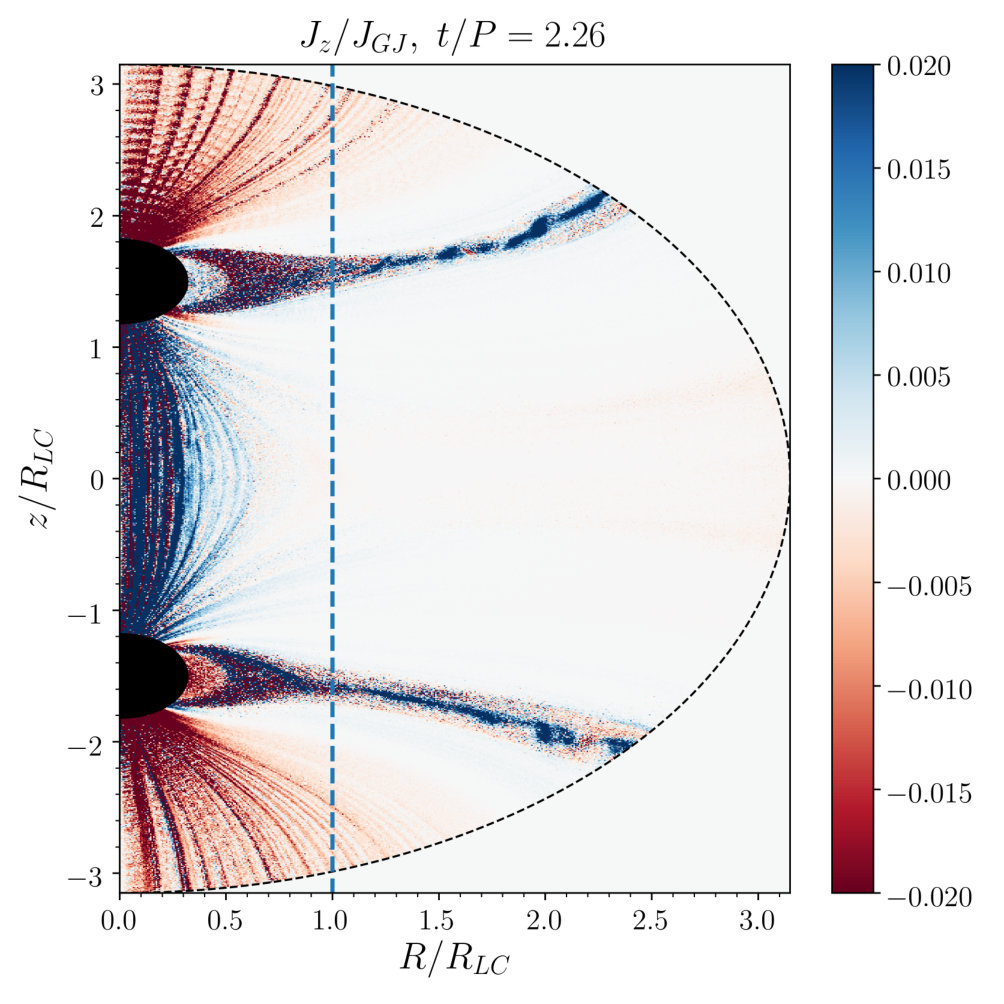 Figure 7
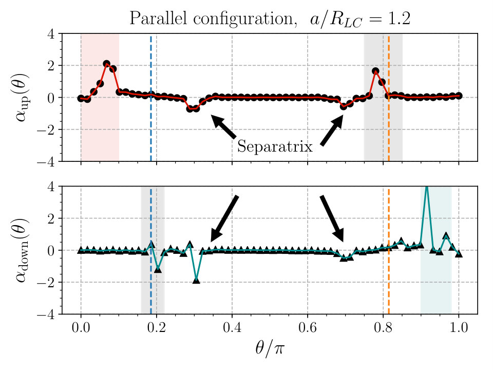 Figure 8
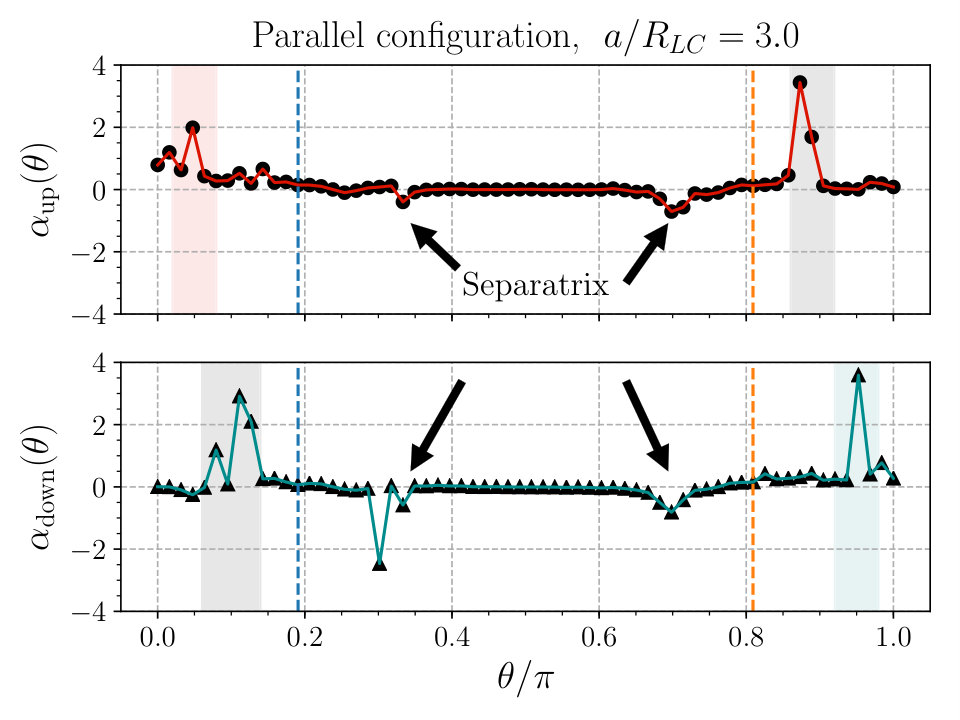 Figure 9
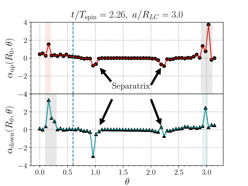 Figure 10
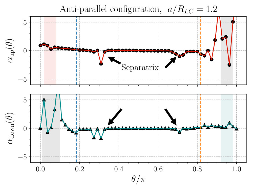 Figure 11
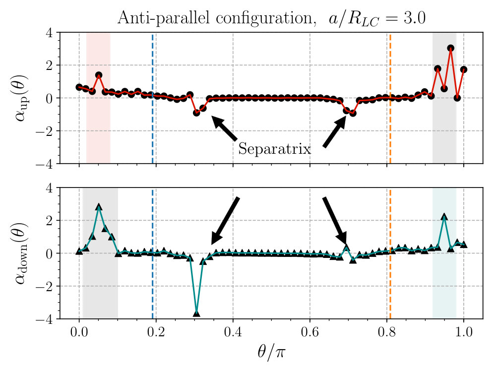 Figure 12
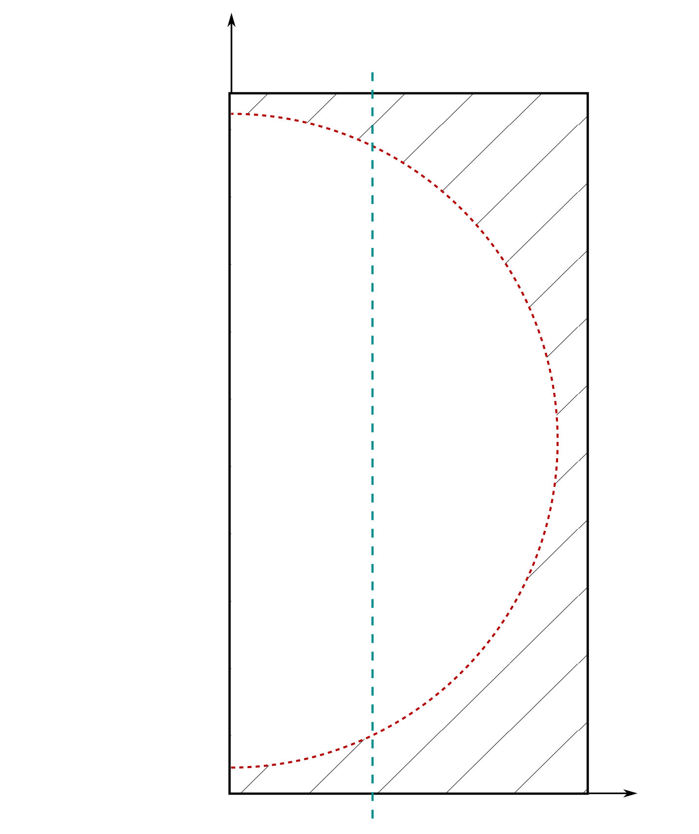 Figure 13
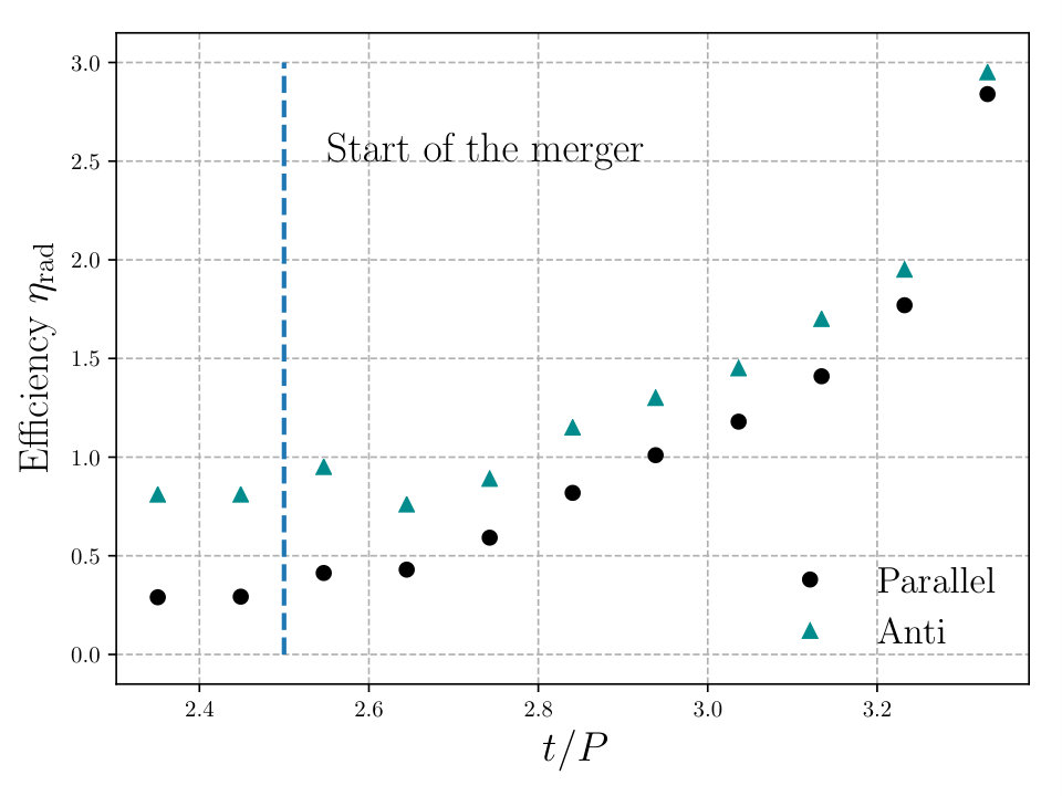 Figure 14
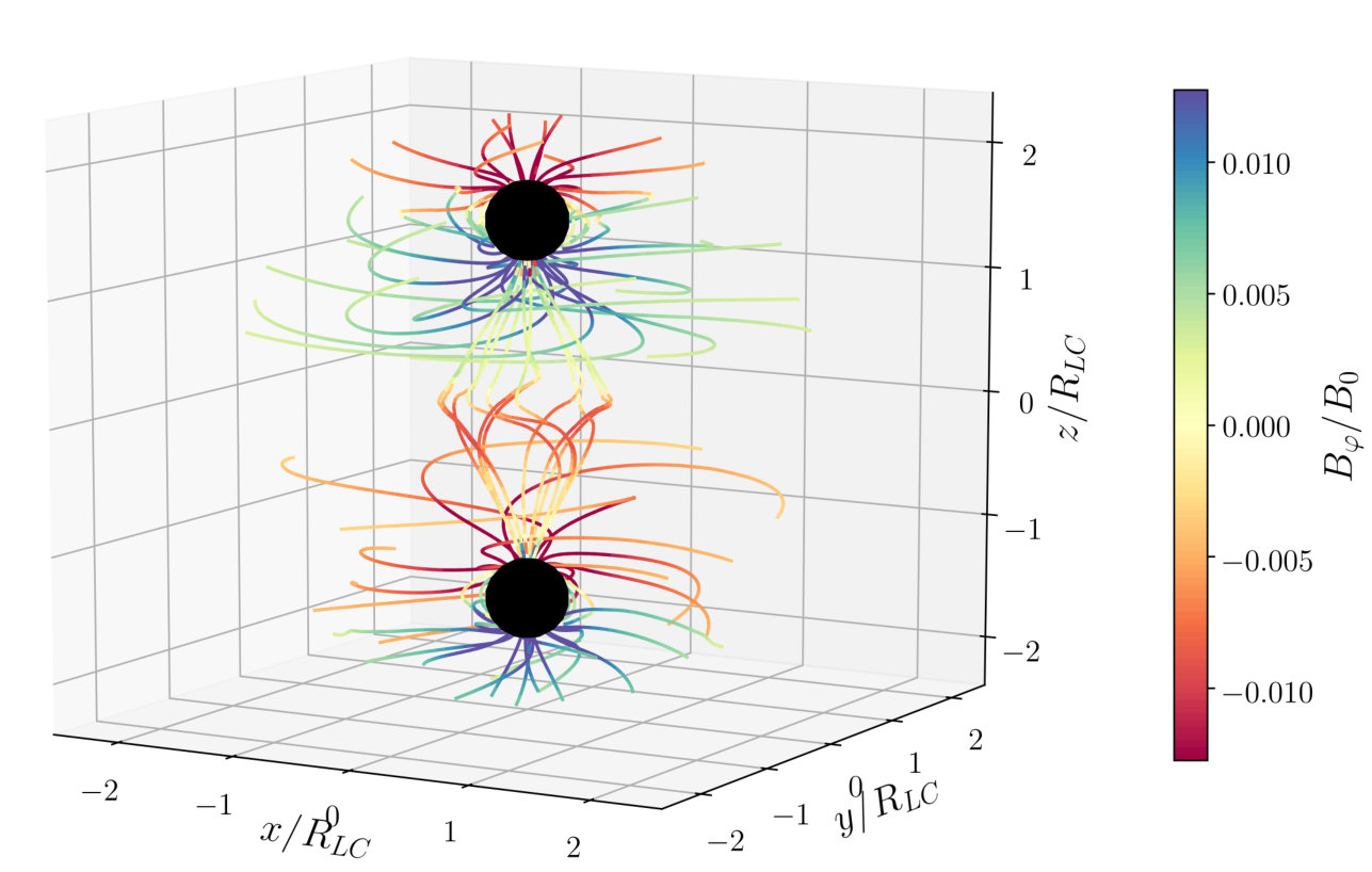 Figure 15
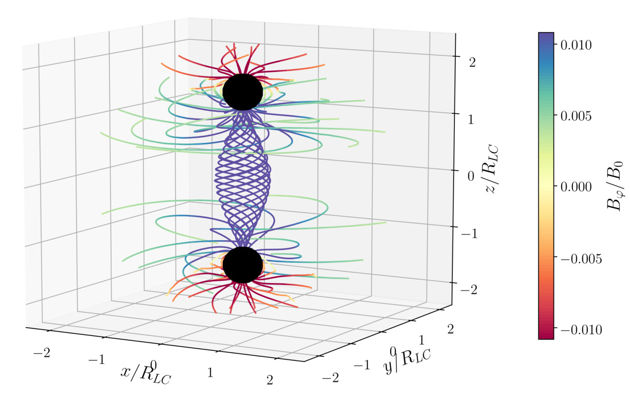 Figure 16
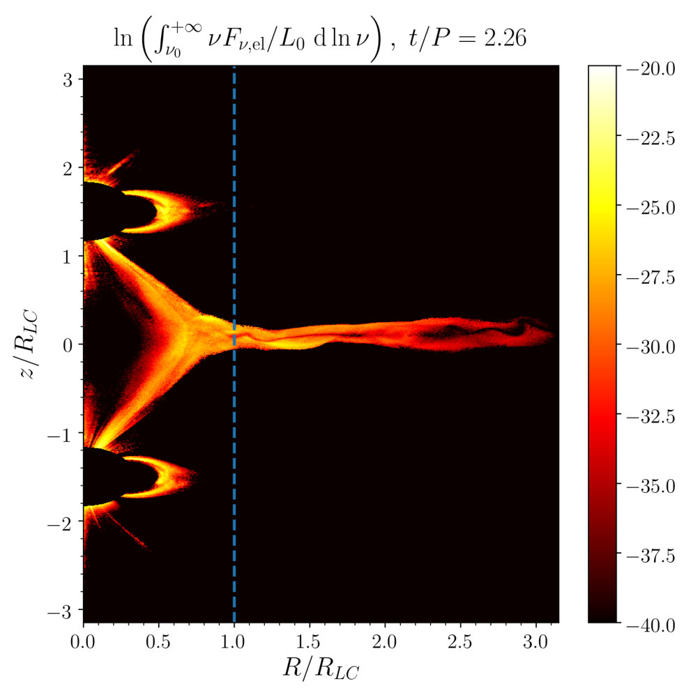 Figure 17
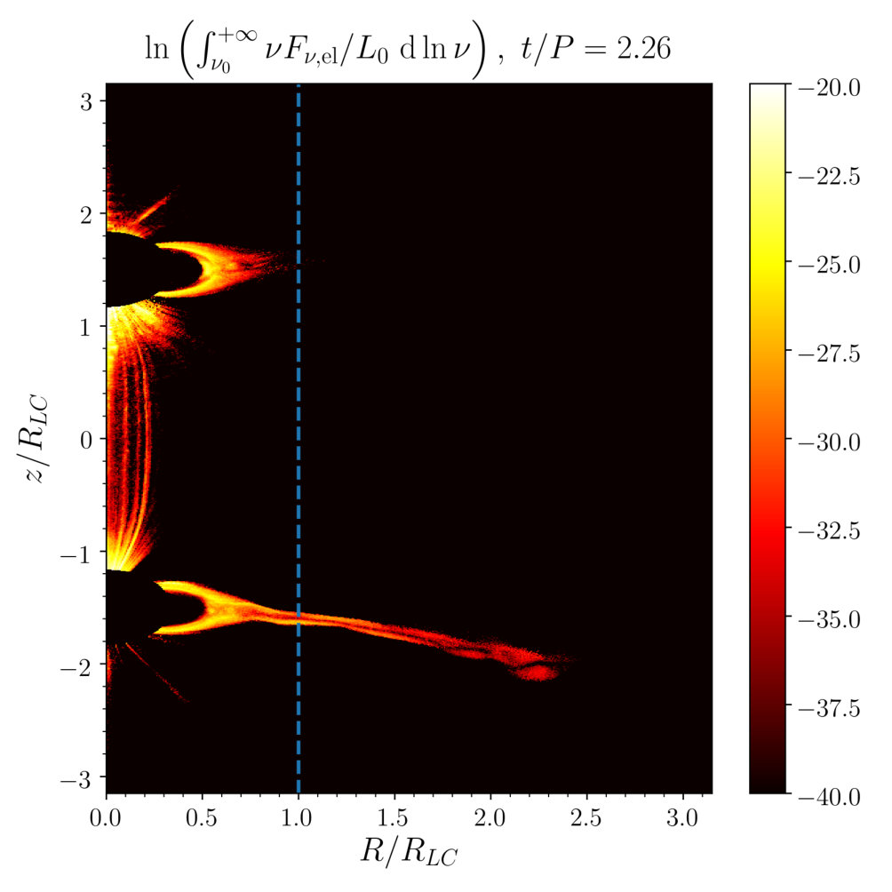 Figure 18
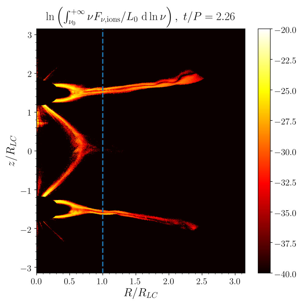 Figure 19
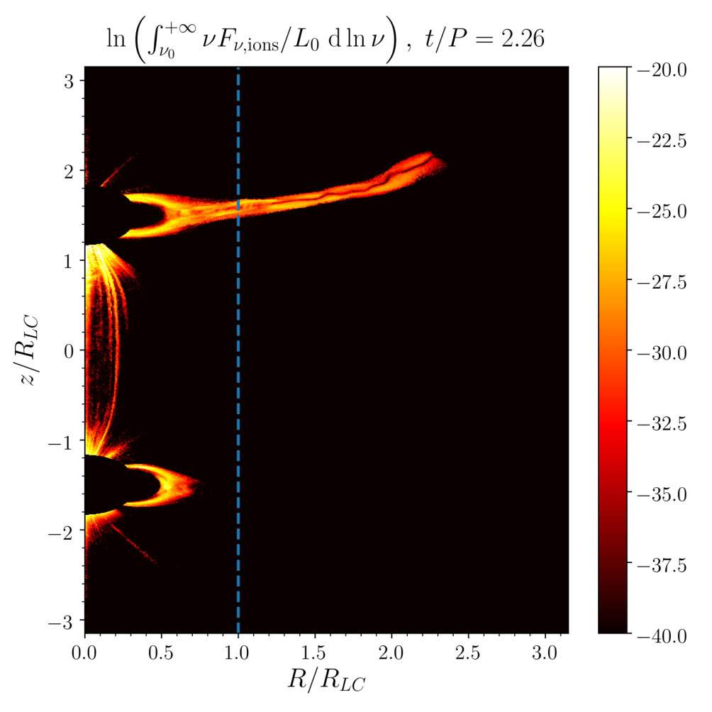 Figure 20
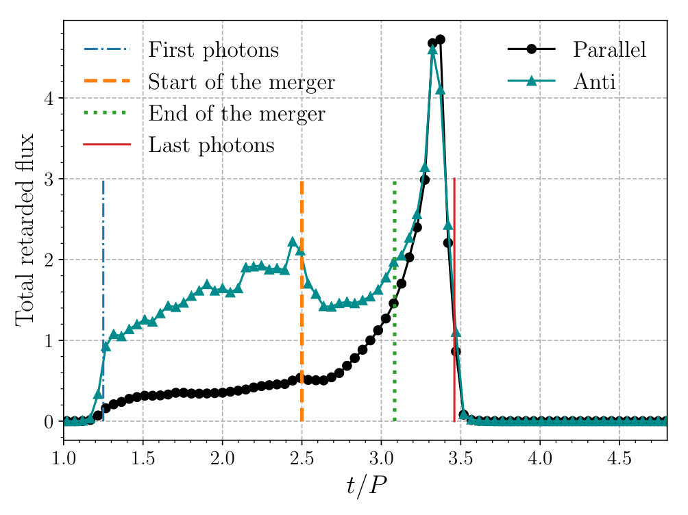 Figure 21
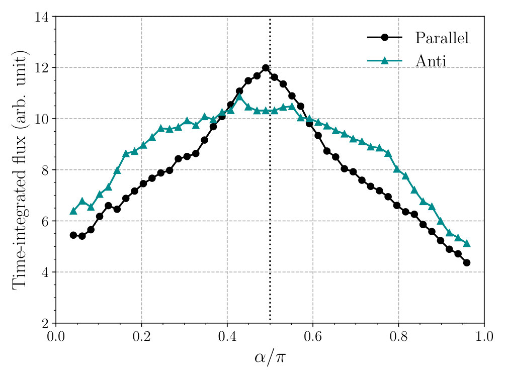 Figure 22
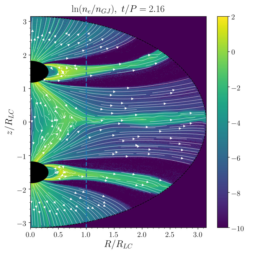 Figure 23
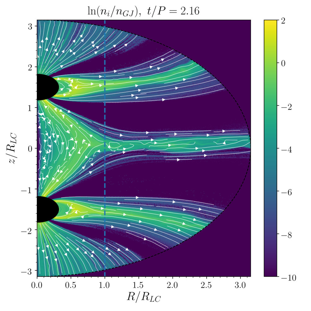 Figure 24
| Parameter | Value |
|---|---|
| Number of cells | |
| Neutron star radius | |
| Injecting shell radius | |
| Skin depth | |
| Larmor frequency | |
| Plasma frequency | |
| Pulsar period | |
| Pair creation threshold | |
| Start of the merger | |
| Initial number of particles per cell | |
| Initial inspiral speed (for ) |
| Separation | Parallel | Anti-parallel |
|---|---|---|
| Symmetric | Asymmetric | |
|---|---|---|
| Same parallel | ||
| Same anti-parallel | ||
| Opposed parallel |
Peer Reviews
No public reviews on file for this paper yet. If you reviewed it on a platform where reviews are public (OpenReview, ICLR, NeurIPS, ICML), you can paste yours below so the community can read it here.
Videos
No videos yet. Explain this paper in a talk, walkthrough, or lecture? Add one.
11institutetext: Univ. Grenoble Alpes, CNRS, IPAG, 38000 Grenoble, France
11email: [email protected]
Kinetic modeling of the electromagnetic precursor from an axisymmetric binary pulsar coalescence
B. Crinquand
B. Cerutti
G. Dubus
(Received 9 November 2018 / Accepted 14 December 2018)
Abstract
*Context. *The recent detection of gravitational waves associated with a binary neutron star merger revives interest in interacting pulsar magnetospheres. Current models predict that a significant amount of magnetic energy should be released prior to the merger, leading to electromagnetic precursor emission.
*Aims. *In this paper, we revisit this problem in the light of the recent progress in kinetic modeling of pulsar magnetospheres. We limit our work to the case of aligned magnetic moments and rotation axes, and thus neglect the orbital motion.
*Methods. *We perform global two-dimensional axisymmetric particle-in-cell simulations of two pulsar magnetospheres merging at a rate consistent with the emission of gravitational waves. Both symmetric and asymmetric systems are investigated.
*Results. *Simulations show a significant enhancement of magnetic dissipation within the magnetospheres as both stars get closer. Even though the magnetospheric configuration depends on the relative orientations of the pulsar spins and magnetic axes, all configurations present nearly the same radiative signature, indicating that a common dissipation mechanism is at work. The relative motion of both pulsars drives magnetic reconnection at the boundary between the two magnetospheres, leading to efficient particle acceleration and high-energy synchrotron emission. Polar-cap discharge is also strongly enhanced in asymmetric configurations, resulting in vigorous pair production and potentially additional high-energy radiation.
*Conclusions. *We observe an increase in the pulsar radiative efficiency by two orders of magnitude over the last orbit before the merger exceeding the spindown power of an isolated pulsar. The expected signal is too weak to be detected at high energies even in the nearby universe. However, if a small fraction of this energy is channeled into radio waves, it could be observed as a non-repeating fast radio burst.
Key Words.:
**pulsars: general – binaries: close – acceleration of particles – magnetic reconnection – methods: numerical **
1 Introduction
On August 2017, the LIGO/Virgo detectors observed a gravitational wave signal that coincided with the measurement of a Short Gamma Ray Burst (SGRB) by the Fermi/GBM instrument (Abbott et al. 2017b). This unique joint detection allowed unambiguous association of SGRBs with binary neutron star mergers (Abbott et al. 2017a).
It is expected on theoretical grounds that these binary systems release a large amount of energy prior to the merger. First developed by Goldreich & Lynden-Bell to explain decametric emission from the Io-Jupiter system (Goldreich & Lynden-Bell 1969), the DC model was recently adapted to other types of astrophysical systems, including binary neutron stars (Piro 2012; Lai 2012). In this framework, the energy dissipation rate can go up to erg/s during the late stage of the inspiral, in the case of neutron stars with high magnetic fields ( G). Some of this energy is then converted into observable radiation. It may partly be consumed by the creation of a plasma “fireball” (Vietri 1996; Hansen & Lyutikov 2001; Metzger & Zivancev 2016). The overall dissipated power predicted by these models is erg/s. In this case, the precursor should be observable from Earth.
The detection of an electromagnetic precursor would be very helpful to trigger multi-wavelength observations of upcoming mergers. Aside from this observational motivation, the interaction of plasma-filled magnetospheres has so far been poorly studied. In particular, it is not known whether the presence of another pulsar can enhance particle acceleration and how it affects pulsar spindown. To investigate a possible electromagnetic precursor to the merger, it is necessary to understand how particles can be accelerated, but the mechanisms at play are too complex to be analytically solved. Magnetohydrodynamic simulations were recently performed to model binary neutron star coalescences (Palenzuela et al. 2013; Dionysopoulou et al. 2015). Although this approach is appropriate to model the overall plasma structure, it fails to capture particle acceleration and cannot produce the shape of the electromagnetic outburst.
In recent years, kinetic modeling of pulsar magnetospheres using particle-in-cell (PIC) simulations has lead to significant progress in our understanding of magnetic dissipation, pair production and particle acceleration (Philippov & Spitkovsky 2014; Chen & Beloborodov 2014; Cerutti et al. 2015; Philippov et al. 2015b; Belyaev 2015; Philippov et al. 2015a; Cerutti & Philippov 2017; Brambilla et al. 2018). In particular, they proved fit to account for the two-peaked structure of gamma-ray pulses (Cerutti et al. 2016b; Philippov & Spitkovsky 2018; Kalapotharakos et al. 2018), and optical polarization properties of the Crab pulses (Cerutti et al. 2016a). Spherical simulations were able to reproduce a quasi force-free magnetosphere and identify magnetic reconnection in the equatorial current sheet as the main acceleration mechanism (Cerutti et al. 2015).
In this work we perform PIC simulations of a merging binary neutron star system in a 2D axisymmetrical cylindrical setup. To retain cylindrical symmetry, we keep both pulsars aligned with the symmetry axis, thus neglecting their relative orbital motion. It is likely that pulsar obliquity decreases with age, as can be seen on theoretical (Philippov et al. 2014) and observational (Tauris & Manchester 1998; Young et al. 2010) grounds (see, however, Beskin et al. 1993). Therefore, it is relevant to study pulsars with aligned magnetic moments and rotation axes. Although the problem is intrinsically 3D, performing 2D simulations allows us to have a much better resolution by decreasing the numerical cost, and to gain physical insight into this complex problem more easily. We explore the mechanisms of particle acceleration resulting from magnetospheric interactions in several configurations. Furthermore, we compute the high-energy radiation lightcurve that would be produced during the inspiral phase of the merger, in order to assess the observability of the precursor. In Sec. 2, we describe the numerical methods and the particular setup we simulate. We also report how the consistency of this new code was tested. The results are presented in Sec. 3.
2 Numerical methods
2.1 Particle-in-cell technique
In this study, we use the relativistic PIC code Zeltron (Cerutti et al. 2013, 2015). In PIC methods, the plasma is treated as a set of charged macro-particles. During one time step three operations must be performed. First, the positions and velocities of the particles are evolved using the Boris push (Birdsall & Langdon 2005). The electromagnetic source terms are then collected on a Yee grid (Yee 1966), using an area weighting procedure. Finally, the fields are updated by solving discretized versions of Maxwell-Ampère’s and Maxwell-Faraday’s equations on the grid. Given the spatial resolution, the time step is enforced by the Courant-Friedrich-Lewy condition (Sironi & Cerutti 2017), so that the numerical scheme remains stable. This scheme does not enforce Maxwell-Gauss’ equation, so the total electric charge deposited on the grid is not conserved. Small errors can accumulate and give rise to nonphysical charge densities. The electric field is therefore corrected every 25 time steps, by solving Poisson’s equation: , where is the charge density, the uncorrected field and the corrected electric field.
Since we intend to model a binary pulsar, the system does no longer retain spherical symmetry, which is natural to consider for an isolated pulsar study. Instead we have implemented a 2D axisymmetric cylindrical version of the code: particles move in a 3D space but all quantities are invariant under rotations about the symmetry axis . Maxwell’s equations are then solved in cylindrical coordinates , where is the distance from the symmetry axis. The simulated domain is defined as , it is centered at the origin. All simulation parameters are given in Tab. 1. The simulated pulsars must have aligned magnetic moments and spin axes. This amounts to neglecting the orbital motion of the two pulsars, which are constantly aligned (see Fig. 1).
2.2 Particles
The numerical setup is presented in Fig. 1. The stellar radius is denoted by . The angular velocity vector and magnetic moment of the top (resp. the bottom) pulsar will be denoted and (resp. and ). They are aligned with the symmetry axis . The simulation starts in complete vacuum, and the stars remain empty of particles at all times. In order to fill the magnetospheres with plasma, electron/positron () pairs are uniformly injected within thin injection shells between and surrounding the stars. Charges with the right sign are then extracted from the surface, while the others rush back to the star. The particle distribution in this shell is reinitialized at every time step, in order to avoid numerical over-densities. These particles are initially corotating with the star, with toroidal velocity . Particles that leave the simulation domain are removed.
The density of the surface plasma is set at the Goldreich-Julian density , where is the polar field strength at the stellar surface (Goldreich & Julian 1969). This is consistent with the actual charge density that is extracted from the star to screen the surface electric fields. The whole electromagnetic cascade, filling the magnetosphere with plasma, is implemented in a simplified way. Following Philippov et al. (2015b), a critical Lorentz factor is empirically defined as a fraction of the maximal energy available to a particle, which is given by the total voltage drop from the pole to the equator at the stellar surface. If a particle reaches a Lorentz factor111In asymmetric simulations we kept the product constant, so that the threshold is unequivocally defined. , and provided the local pair plasma multiplicity (defined as the ratio between the plasma density and the Goldreich-Julian density) remains smaller than , an pair is created at the location of the parent particle, whose energy is consequently reduced. The resulting pair carries a fixed fraction of the parent particle’s energy. The factor was chosen so as to sufficiently fill the magnetosphere and reach a force-free regime (Cerutti & Beloborodov 2017). This was checked by comparing the spindown of a single pulsar to the expected values in the monopole and dipole cases. Some numerical problems arise because of the discretization of the pulsar sphere by Cartesian cells in the plane. For example, it can cause important angular inhomogeneities in the plasma injection, which impact the whole magnetosphere. This difficulty is circumvented by moderately increasing the thickness of the injecting shell and the number of macro-particles per cell.
2.3 Electromagnetic fields
In most simulations (see Sec. 3.5 for asymmetric simulations with and ), and have the same magnitude, so both pulsars have the same light cylinder . The two pulsars are initially separated by a distance , and disposed symmetrically with respect to the origin. The initial magnetic field is the sum of two dipole fields generated by each pulsar. As the simulation proceeds, this field is enforced inside the stars (for , with the distance from the center of pulsar ’’). Pulsar spin is implemented by imposing a poloidal electric field within the pulsar (for ), given by
[TABLE]
arising in the laboratory frame because the electric field is zero in the corotating frame, assuming that the neutron star interior is perfectly conducting. The toroidal electric field in the star is set to zero. In order to mimic an open outer boundary, a numerical resistivity (where is the distance from the origin) is given to the medium for , with . This amounts to adding a resistive term to Maxwell’s equations: for instance Maxwell-Faraday’s equation becomes . In this part of the simulated domain the fields are critically damped. The chosen resistivity profile is chosen to be smooth, so as to avoid unwanted reflections (Cerutti et al. 2015):
[TABLE]
On the outer boundaries, a zero-gradient condition is enforced. Cylindrical symmetry requires the radial () and toroidal ( fields to be zero on the symmetry axis, whereas the vertical () components have no gradient on the axis. The correction potential is set to zero inside the pulsars, with an additional zero-gradient condition for the electric field at the stellar surfaces.
Initially, the electric field is zero everywhere but in the pulsar. A simulation starts with the launching of a spherical wave distributing the electric field in the domain. If the toroidal magnetic field is set to zero for , the simulation cannot start properly. On the other hand, if is simply left free to evolve, some spurious grows at a slow but constant rate inside the injection shell. This is due to a round-off error in the computation of the component of in the shell (), which is supposed to be zero inside the star. This problem does not occur in spherical coordinates, because it is sufficient to use a single radial cell as an injection domain. In this cylindrical setup the shell must be several cells wide to enable homogeneous plasma injection. To alleviate this difficulty, a resistivity profile similar to Eq. (2) was given to the injection shell, where was left free to evolve. The induced damping rate was chosen to be slightly greater than the spurious growth rate.
2.4 Pulsar separation
Since the orbiting binary pulsar loses energy because of gravitational wave emission, the two stars get closer and closer. The orbital motion of the stars was not simulated, but the analytical expression for the separation between them was implemented ad hoc. For a binary star with masses , , separated by a distance , the rate of energy loss is given by (Carroll 2003):
[TABLE]
Injecting the gravitational energy of a two-body system and solving the associated differential equation yields:
[TABLE]
where is the initial separation. Numerical evaluation for the inspiral time yields
[TABLE]
The inspiral time was rescaled so as to match the code units, with .
The inspiral begins in the simulation only once both magnetospheres have been filled with plasma and have reached a quasi-steady state (the topology of the magnetosphere and the field strength no longer vary), which usually requires about rotation periods. Once this phase has elapsed, the pulsar separation decreases according to Eq. (4). The simulation ends when the pulsars touch. Otherwise, no general relativity effect was included in the simulation.
2.5 Modeling radiation
In order to evaluate the electromagnetic signature of the merger, the radiation of accelerated particles must be computed. The procedure is described in Cerutti et al. (2016b). Particles essentially cool through synchrotron radiation. The radiated power spectrum emitted by a single particle with Lorentz factor moving in a perpendicular magnetic field in the ultra-relativistic limit is (Blumenthal & Gould 1970):
[TABLE]
where is the modified Bessel function of order . The critical frequency is given by
[TABLE]
In the presence of an electric field, a standard procedure consists in replacing the perpendicular magnetic field by an effective field strength (Kelner et al. 2015; Cerutti et al. 2016b):
[TABLE]
This procedure is valid only in the ultra-relativistic limit, with , and takes into account both synchrotron and curvature radiation. This procedure allows one to deal with the drift. Indeed, in the wind zone, the motion of the plasma is dominated by this drift. Injecting the drift velocity into Eq. (8) yields . Physically, the plasma does not radiate much when the flow is dominated by the drift, because in the drift frame where the electric field is zero the magnetic field strength is reduced by a factor , the Lorentz factor of the bulk flow. Keeping the actual instead of the effective field would lead to highly overestimated synchrotron losses.
Moving charged particles emit “macro-photons” along their direction of motion. This is only valid in the ultra-relativistic limit, as the emission cone has a semi-aperture angle . Once emitted, these photons escape the simulation (unless they hit a star). Each macro-photon conveys a power spectrum given by (6). The output of the code is , where is the locally emitted power spectrum. In order to find the high-energy emission sites, the code outputs , where is a typical synchrotron frequency. In this 2D axisymmetric setup the spherical surface of a pulsar must be discretized in Cartesian coordinates (see Sects 2.2 and 2.3). Right at the stellar surface, fields suffer discontinuities that produce spurious particle acceleration. Consequently, we choose to discard macro-photons emitted within of the stellar surfaces. Similarly, particles that would undergo nonphysically high accelerations near the surfaces are also removed from the simulation.
The emitted macro-photons are collected at infinity, making an angle with the symmetry axis. The propagation time of the photons depends on the location of its emitting particle and its direction of motion. The time delay between a photon emitted at polar coordinates in the plane, propagating with an angle with respect to the symmetry axis, and one emitted at the origin in the same direction, is given by:
[TABLE]
All photons emitted at a given time step are distributed on a grid according to their time delay. Since the merger is inherently unsteady, we collect photons every 10 time steps.
2.6 Consistency checks
Since PIC simulations of pulsar magnetospheres had not yet been conducted in cylindrical coordinates, we checked that the output of the code against previous results. Some analytical solutions are known for an isolated pulsar magnetosphere. First, the electromagnetic solver alone was tested in vacuum. For a monopolar field , the electric field can be readily computed in spherical coordinates in the whole space (Cerutti & Beloborodov 2017; Jackson 1998), using the boundary condition at given by Eq. (1):
[TABLE]
The simulated electric field of an empty magnetosphere was found to be consistent with Eq. (12), the angular and radial dependence agreeing with this theoretical prediction. The toroidal field remained zero in the steady state. The code was then tested on a monopole force-free magnetosphere, for which an analytical solution also exists (Michel 1973a, b; Henriksen & Rayburn 1971). In the presence of plasma a toroidal field develops, given by
[TABLE]
We recovered this behaviour with good accuracy. Finally, the single force-free aligned dipole configuration was also simulated. The spindown power of the dipole pulsar can be analytically estimated (Cerutti & Beloborodov 2017) to scale like
[TABLE]
where is the equatorial surface field of the pulsar. This served as another quantitative test for the 2D-axisymmetric code. Previous 2D spherical simulations (Cerutti et al. 2015; Belyaev 2015) showed that the outgoing Poynting flux indeed scales like , provided the force-free regime is achieved. If the pair creation parameters are properly adjusted, so as to reach a force-free regime, we confirm this result in the axisymmetric setup. The quantity provides a useful reference to convert energy flux from code units to physical units.
3 Results
Aside from Sec. 3.5, both pulsars have equal magnetic field strengths and rotation periods in the following. We first present simulations that have reached a quasi-steady state, in order to study the magnetospheric interactions at play. In Secs. 3.4 and 3.5 we then study the inspiral phase and the resulting electromagnetic outburst.
3.1 Magnetospheric structure
Eight configurations can be simulated with this axisymmetric setup, depending on the relative orientations of the magnetic moments and the rotation axes. We focus on the four configurations where the pulsars have their magnetic moments parallel or anti-parallel, and their rotation axes parallel or anti-parallel. The top pulsar has and , whereas the bottom pulsar can have its magnetic moment or rotation axis reversed. Until Sec. 3.5 we only study the two configurations with the magnetic moments aligned for both stars. Indeed, symmetric simulations with opposed magnetic moments are qualitatively similar, regardless of the relative spin orientation (this is not shown in the symmetric case, but see Sec. 3.5). The two opposed dipolar fields exclude one another, so no field line links the pulsars, and no reconnection layer occurs in between.
3.1.1 Parallel configuration
Fig. 2 shows the steady state toroidal magnetic field. Since the two pulsars have no relative motion before the merger is initiated, a large zone between them remains closed, with no outflowing currents and no toroidal fields. The main feature of this configuration is the equatorial sheet, that supports a discontinuity in the toroidal (like in the isolated pulsar case) and poloidal field. A discontinuity in the toroidal field induces a radial current sheet, visible in Fig. 2. Note that this “inter-pulsar” current sheet qualitatively differs from the “proper” current sheets. Indeed, it carries a current with the opposite sign, which means electrons undergo greater acceleration than with a single pulsar. It is a third promising site for particle acceleration, apart from the two proper current sheets. The location of the Y-point of this current sheet is determined exclusively by the separation between the pulsars, rather than the light cylinder. This means that unlike the isolated pulsar configuration, here reconnection occurs well within the light cylinder where the fields are much stronger, although this is more obvious at closer separations. The field lines are represented in three dimensions in Fig. 4.
Densities for the two species are shown in Fig. 6, as well as the bulk velocity field lines. The small discrepancies between the electronic and positronic densities imply that the plasma is globally quasi-neutral, except in the closed zones and within the current sheets. Some density gaps are visible surrounding the current sheets, as in Philippov et al. (2015b). In the wind zone, the solution resembles Michel’s split monopole (Michel 1973a). The bulk velocity field is similar for both species in the wind zone, where it is approximately radial, as prescribed by the drift velocity of the particles. A difference can be found in the inter-pulsar current sheet for instance: electrons flow outward whereas positrons move back towards the pulsars.
3.1.2 Anti-parallel configuration
The initial magnetic field is the same as in the parallel case, but here the two stars spin in opposite directions. Consequently, the field lines linking the two stars are twisted (see Fig. 5), while a strong toroidal field develops in between, as can be seen in Fig. 3. We can relate this configuration to the DC model (Lai 2012; Piro 2012) which considers a magnetic neutron star orbiting a non-magnetic but perfectly conducting companion. The motion of the non-magnetic star with respect to the magnetic field of the primary induces an electromotive force, which in turn drives currents along the magnetic field lines emerging from the magnetic star. The energy is dissipated because of the plasma and stellar resistivity. This model allows us to shed light on this magnetic configuration: the toroidal field between the pulsars induces a strong current flowing from the down pulsar to the top, as can be seen in Fig. 3. No instability prevents from growing in these 2D simulations.
In both configurations, the single pulsar current sheets seem to be repelled from the midway equator, although they both carry opposite electric charges. This is a magnetic pressure effect. The presence of another pulsar generates a stronger toroidal field outside the light cylinder, which induces a magnetic pressure acting perpendicular to the field lines. The equilibrium position of the current sheets results from a balance between magnetic and kinetic plasma pressure. Close to the outer boundary, the current sheets become unstable due to the kink instability. It is also subject to the tearing instability. Magnetic islands are generated at the Y-point, then advected away (see Fig. 2).
The latitudinal stripes visible in Figs. 2 and 3 likely stem from the discretization of the sphere, as mentioned in Sec. 2.2, and should not be considered physical. However, the radial current oscillations have a physical basis. If some unscreened parallel electric field lies at the stellar surface, particles are accelerated and induce pair creation. Then the local plasma density rises, so the electric field is momentarily screened and particle acceleration is quenched. As the plasma flows away, the same process starts again, giving rise to these oscillations.
3.2 Spindown
The interaction between the two pulsars significantly impacts their spindown. Two steady state simulations were performed, with and . We compute the Poynting energy flux flowing out of each pulsar at separately, then we sum the results to get the total luminosity . This is compared to the Poynting flux flowing out of the simulation , through a sphere of radius centered on the origin. The dissipation rate is then computed as . The results are shown in Tab. 2. The spindown values lie between and , being the spindown of an isolated pulsar (14). If the separation tends to infinity, the spindown will be . If tends to [math], the magnetic moment of the star will double and its spindown will quadruple. For intermediate separations, one pulsar can intercept outgoing field lines from the other, thus reducing its Poynting flux.
At fixed separation, the anti-parallel total spindown is higher than the parallel spindown. The spindown does not increase when decreases in the parallel case because the presence of another pulsar does not significantly affect the magnitude of the toroidal field (since they have opposite polarities), and the Poynting flux approximately scales like . More field lines outgoing from one pulsar are captured by the other, diminishing the amount of energy extracted along the open field lines. On the other hand, in the anti-parallel configuration the toroidal field is amplified near the stars, which leads to a higher Poynting flux.
The fraction of dissipated spindown increases as the separation decreases. It is greater in the parallel configuration. This fact seems to support the idea that the inter-pulsar current sheet is a prominent site for dissipation and particle acceleration. The absence of this layer in the anti-parallel configuration could imply that the DC mechanism is a less efficient dissipation mechanism than magnetic reconnection. However, the amplification of the toroidal field in this configuration compensates for this effect.
3.3 Particle acceleration and high-energy radiation
The sites of pair creation can be investigated through the local quantity , where is the (spherically) radial current flowing out of a pulsar, the polar angle defined with respect to this pulsar, and the Goldreich-Julian charge density. If , the charge-separated current escaping from the star fails to sustain the current required by the current sheet, so a parallel electric field develops which accelerates particles and produces pairs (Beloborodov 2008). Pair creation must occur to supply current. This diagnostic was computed for both the up and down pulsars, following Parfrey et al. (2012).
The anti-parallel configuration is presented in Fig. 7. The presence of the second pulsar greatly increases , which can reach values from to at the south pole of the top pulsar and at the north pole of the bottom pulsar (the “inward” poles). This is consistent with the DC model: the electromotive force between the stars drives a large current flowing from the down to the up pulsar. Pair creation is extremely efficient in between the pulsars, hence the formation of a dense pair plasma. However, this plasma remains highly magnetized and does not radiate much. At closer separation, the locations of the peaks in are almost unchanged, whereas the magnitude of the inward pole peaks rises a lot. Fig. 7 shows the same diagnostic for the parallel configuration. Here, the magnitudes of the inward pole peaks and outward pole peaks are similar. At closer separation, the inward pole peaks move towards the stellar equators.
In both cases, pair creation seems to be slightly enhanced at the outward poles with respect to the isolated pulsar, remaining close to . Indeed, this is why periodic oscillations in current density can occur at the poles in Figs. 2 and 3. We also find that the closed zone gets smaller and the polar cap larger. This is proven by the fact that the return current sheets ( marks the location of the separatrix, separating closed field lines from open ones) are located closer to the equator and further from the theoretical polar cap angles and , where is given by
[TABLE]
This likely results from the magnetic pressure exerted by the other pulsar. This effect is more significant in asymmetric simulations (see Sec. 3.5).
The high-energy radiation maps for electrons and positrons are shown in Figs. 8, 8 for the parallel configuration, Figs. 8 and 8 for the anti-parallel configuration. As mentioned earlier, particles too close to the stellar surface are spurious and should not contribute to the radiation diagnostic. The anti-parallel maps show that at large separation, high-energy radiation is mainly due to the current sheets proper to each pulsar. Besides, in accordance with the diagnostic of Fig. 7, particle acceleration is enhanced at the inward poles, with respect to the outward polar cap emission. In the parallel configuration, the inter-pulsar current sheet radiates predominantly, as expected since the Y-point lies within the light cylinder where the field is stronger. From the radiation data, one can infer how much of the spindown was channeled to electromagnetic radiation, by computing the total radiative efficiency in the total simulation domain (excluding a thin shell of width at the stellar surface):
[TABLE]
In this study, the radiative efficiency of an isolated pulsar is . The emitted radiation in the steady state two-pulsar setup is much more intense than in the isolated pulsar case. At , we find in the parallel configuration and in the anti-parallel configuration. At the closer separation , the efficiencies are and respectively.
To sum up, even though the reconnection mechanism is more efficient at dissipating electromagnetic energy than the DC mechanism, the amplification of in the anti-parallel configuration compensates for its relative inefficiency. The amount of dissipated energy is similar in both cases (around at , inferred from Tab. 2). Eventually, the radiative efficiency increases faster with decreasing separation in the anti-parallel configuration. This can be explained by the low densities achieved in the inter-pulsar reconnection layer, with respect to the dense zone between the stars. Although particles experience greater accelerations in the parallel configuration, this affects a smaller number of particles, so that in fine more energy is converted into particle kinetic energy in the anti-parallel configuration.
3.4 The inspiral phase
The lightcurves obtained using the procedure described in Sec. 2.5 are presented in Fig. 9. In these simulations, the computation of the lightcurves started after (marked by a dash-dotted line on Fig. 9), while the inspiral was initialized at (marked by a dashed line). Computing the lightcurve after a steady state is reached provides a baseline to evaluate the increase in the measured flux, and makes it possible to check that the routine works correctly by comparing the steady state value to the radiative efficiency.
The two curves are qualitatively different before the inspiral starts. In the parallel simulation, a steady state is reached when the merger is initiated. Conversely, the anti-parallel lightcurve has not yet reached a steady state when we start approaching the stars. The received flux rises steadily. The regular increase in radiated flux is due to the accumulation of toroidal field between the pulsars. This can be confronted with the DC model mentioned earlier. Lai (2012) noticed that flux tubes twisted beyond break down, because the magnetic pressure exerted by the toroidal field is too large. This occurs if the resistivity of the plasma is too low, and the currents too high. The axisymmetry of the tube is broken by unstable kink modes, which distort the tube. Nonlinear evolution of the tube disrupts it completely. Magnetic energy is then dissipated by reconnection. Thus a quasi-periodic circuit can be expected: after the flux tube breaks, reconnection between the inflated field lines restores the linkage between the two stars and the cycle repeats. However, this phenomenon can only be captured in 3D simulations. The staircase look of the anti-parallel lightcurve possibly results from a discharge phenomenon similar to what was explained in Sec. 3.1. Nonetheless, the presence of such twist in 2D simulations is promising as to the strength of the outburst, since even more energy should be released by the breaking of the flux tube.
After the merger starts, both curves eventually meet. The peak of the lightcurve is reached after the end of the merger (marked by the dotted line in Fig. 9). The full width at half maximum of the peak is . This can be compared to the final orbital frequency in the GW170817 neutron star merger 400\text{,}\mathrm{Hz}$$ (Abbott et al. 2017a, b). This means that the energy of the magnetospheric outburst is released during the last orbit of the binary. The angular distribution of the pulse is shown in Fig. 10. The radiation is mainly emitted in the equatorial plane in both configurations, although the signal is not strongly anisotropic. Consequently, the direction of the line of sight is not critical regarding observability. The anti-parallel angular distribution is broader than the parallel one, because the emission mechanism occurring before the merger is different. In contrast to magnetic reconnection, which mainly accelerates particles near the equatorial plane, in the anti-parallel configuration particles are accelerated when heading from one pulsar to the other, thus pointing towards high latitudes.
The similarity between the two lightcurves in the late phase strongly indicates that close to the merger, the physics that accelerates particles and dissipates energy is the same. In both configurations, there is a toroidal current sheet resulting from the discontinuity in the poloidal magnetic field. At high separations its effect is negligible with respect to the other current sheets (the proper pulsar current sheets, or the inter-pulsar radial current sheet in the parallel configuration). However, as the pulsars close up, it becomes predominant in both cases because the poloidal field dominates over the toroidal component. The snapshots of right before the pulsars touch show that the toroidal sheet is indeed predominant, and that it has a similar shape in both configurations. At the end of the inspiral, dissipation mainly occurs in the toroidal current sheet through magnetic reconnection, which converts a great amount of energy, as the fields so close to the stars are huge. Plus, magnetic reconnection is forced as the pulsars close up, which increases the reconnection rate.
At the end of the day, the pulsar inspiral leads to a great increase in radiated power. The instantaneous radiative efficiency (displayed in Fig. 11) shows an increase by a factor of the bolometric luminosity for both configurations between the beginning and the end of the inspiral phase. This amounts to an increase by a factor with respect to the case of two quasi-isolated pulsars, with . Even so, the dissipated power is well below the previous theoretical expectations from the DC model. Including the orbital motion in 3D simulations would probably increase the simulated dissipated energy, as the relative motion and thus the electromotive force would be greater. However, these theoretical estimates concern the total output energy, yet only the radiated energy will leave an observable signature.
3.5 Asymmetric simulations
So far we have focused on symmetric binaries. Actual binary pulsars are likely to be asymmetric (Tauris et al. 2017; Piro 2012), comprising a recycled pulsar spinning rapidly and a younger, slower pulsar with a stronger magnetic field. This was confirmed by the discovery of the double pulsar J0737-3039A/B (Kramer & Stairs 2008), for which and . However, such ratios are far too extreme for our setup. The light cylinders of both pulsars must be included in the simulation domain, otherwise the closed magnetic field lines of the slow pulsar interact with the outer damping layer. In this case the closed corotating zone is artificially reduced, which induces spurious particle acceleration. Instead, we performed simulations with and , and increased the size of the box to include the whole magnetosphere of the slow pulsar. The bottom pulsar is the old recycled pulsar; it has the same spin and magnetic strength than in the symmetric simulations, whereas the top pulsar has a stronger field and slower spin.
A map of the normalized toroidal field in the configuration with aligned spins and magnetic moments is shown in Fig. 12. In contrast to symmetric simulations, the relative orientations of the spins matter little. The parallel and anti-parallel configurations are similar, since the toroidal field of the fast recycled pulsar dominates anyway. Strongly twisted magnetic field lines connect the two pulsars, like in the symmetric anti-parallel setup. The closed zone of the weak pulsar is compressed because of the influence of the strong one above it. The inter-pulsar current sheet present in the symmetric parallel configuration (see Fig. 2) is missing in Fig. 12. Snapshots of the toroidal field at early times show that these two current sheets merge, as the toroidal field of the fast pulsar takes over. The resulting current sheet is deflected upwards in this parallel configuration, but downwards if they are anti-parallel. This is because the compensation of the top pulsar toroidal field makes the magnetic pressure initially smaller above the down pulsar than below.
In this situation it is interesting to study also the case of two opposed magnetic moments. As shown in Fig. 12, the situation is quite different. No field line can connect the two stars, so the influence of the strong pulsar on the weak one can only be indirect. Plus, no current can flow from one pulsar to the other. As a result, the relative orientation of the spins has rigorously no impact on the magnetic topology, the polarities of the toroidal field and currents due to the down pulsar are simply reversed. At , the magnetosphere of the weak pulsar is confined within the strong field of the other one. Its magnetic field lines then open up and extend to infinity as rotation is imposed. The current sheet of the weak pulsar is strongly deflected. Remarkably, at high separations, this configuration radiates no more than the isolated pulsar. However, after the merger starts, the radiated flux strongly increases by a factor , until it reaches usual outburst values (see Tab. 3).
We identify multiple dissipation mechanisms. Magnetic reconnection occurs at the Y-point of the current sheet, which is pushed closer to the star by the strong pulsar. In the case of aligned magnetic moments, strong pair creation and particle acceleration occur between the pulsars, as in the symmetric anti-parallel configuration. The higher outburst values in asymmetric simulations can be understood in this framework (see Tab. 3). Asymmetric simulations exhibit an intense magnetic field, which compresses the old pulsar’s magnetosphere. The Y-point at the foot of the recycled pulsar’s proper current sheet lies within its light cylinder. Reconnection is therefore more efficient than in symmetric simulations. We also think that in contrast to symmetric simulations, emission from the north polar cap of the strong pulsar may be essential. High-energy emission in this area has very contrasted stripes, which indicates a violent pair creation cascade. The presence of the fast pulsar below implies strong currents must flow from the south polar cap of the strong pulsar. Therefore strong currents must also flow from its north polar cap, and pair creation is triggered to supply them. Then the huge surface parallel electric field accelerates particles. This last mechanism was negligible in symmetric simulations. However, the radiation diagnostics in the asymmetric simulations must be taken with care. Since the magnetic field of the top pulsar is increased in this setup, the plasma quantities are less resolved, and the output data is not fully reliable close to the pulsars. The exact acceleration processes are thus harder to infer.
4 Discussion, observational prospects
We have performed global PIC simulations of a binary pulsar, with various magnetic moments and spins. Our strongest conclusion is that the total radiated power increases by two orders of magnitude during the whole inspiral. The bolometric luminosity can reach up to ten times the spindown power of an isolated pulsar. The lightcurve presents a peak whose width is roughly , which approximately corresponds to the last orbit of the double pulsar. The shape of the peak depends very little on the relative orientation of the spins or magnetic moments. The radiative power is concentrated within the equatorial regions but presents a weak anisotropy. We find that magnetic reconnection is a key ingredient in for particle acceleration and the emission of high-energy synchrotron radiation in all the configurations explored here. In the symmetric configuration, dissipation occurs mainly because of an inter-pulsar current sheet forming at the interface between the two pulsar magnetospheres. As a result, electromagnetic energy is released even in the case where the two pulsars spin synchronously. Before the last stage of the merger, a significant amount of energy is also dissipated between the two stars in the symmetric anti-parallel configuration. Besides, pair creation at the outward poles is amplified with respect to the isolated pulsar configuration. In particular, in asymmetric simulations, pair creation in the vicinity of the slow magnetized pulsar is revived by the presence of the fast-spinning pulsar.
A natural extension of this work would be to perform 3D PIC simulations of a binary aligned pulsar, and more generally with arbitrary inclinations. This would have several benefits. First, we would be able to capture plasma instabilities that can only develop in 3D. For instance, the symmetric anti-parallel configuration displays a highly twisted flux tube, which should be unstable in a 3D setup. This could be another source of energy dissipation. Second, a 3D setup would allows us to simulate more realistic configurations. But more importantly, we would be able to take orbital motion into account. Since the orbital frequency peaks at the merger, it might lead to an increased electromotive force, stronger currents and more dissipation. The luminosity of the precursor predicted here should therefore be seen as a lower limit. Notwithstanding this, for the first time we are able to self-consistently solve the magnetospheric interaction between two coalescing pulsars. This simplified setup allows us to handily elucidate the physical mechanisms at play.
Assuming a binary pulsar with a powerful Crab-like pulsar (Bühler & Blandford 2014), we predict a luminosity for the electromagnetic precursor of its coalescence of erg/s. In the optimistic case where most of this energy is emitted in the Fermi/GBM range, this sets a distance upper limit of Mpc for detection. Thus, only the local group galaxies could be probed this way. For comparison, the neutron star merger event GRB 170817A, which occurred at a distance of Mpc, released an amount of erg/s in the range (Abbott et al. 2017a). The situation is similarly grim in X-ray, but radio emission could be of better use. Some radio detectors such as MeerKAT, or the SKA array in a near future, map the whole sky in real time with high sensitivity. There are some caveats however: the radio luminosity of most pulsars is only a small faction of the spindown power (usually around ). Dispersion by the interstellar medium is also likely to delay the arrival of the radio burst, which cannot arrive ahead of the merger. Besides, radio emission is coherent and does not directly originate from particle acceleration, but may rather be related to pair creation (Philippov et al. 2015a). Although we observe a strong pair creation cascade at the polar caps, especially during the inspiral phase, we are not able to compute the radio efficiency of the binary. Still, radio detection is a promising candidate for the prospects of neutron star merger observability. In particular, Fast Radio Bursts have duration and energy range consistent with pulsar coalescences, and could be counterparts to non-repeating events (Pen 2018).
Acknowledgements.
We would like to thank the referee Richard Henriksen for valuable comments on the manuscript. We acknowledge the support from CNES and the Université Grenoble Alpes (IDEX-IRS grant). This work was granted access to the HPC resources of CINES on Occigen under the allocation A0030407669 made by GENCI.
The reference list from the paper itself. Each links out to its DOI / PubMed record.
- 1Abbott et al. (2017 a) Abbott, B. P., Abbott, R., Abbott, T. D., et al. 2017 a, Ap J, 848, L 13
- 2Abbott et al. (2017 b) Abbott, B. P., Abbott, R., Abbott, T. D., et al. 2017 b, Physical Review Letters, 119, 161101
- 3Beloborodov (2008) Beloborodov, A. M. 2008, Ap J, 683, L 41
- 4Belyaev (2015) Belyaev, M. A. 2015, MNRAS, 449, 2759
- 5Beskin et al. (1993) Beskin, V. S., Gurevich, A. V., & Istomin, Y. N. 1993, Physics of the pulsar magnetosphere
- 6Birdsall & Langdon (2005) Birdsall, C. K. & Langdon, A. B. 2005, Plasma Physics via Computer Simulation, 1st edn. (Taylor & Francis)
- 7Blumenthal & Gould (1970) Blumenthal, G. R. & Gould, R. J. 1970, Reviews of Modern Physics, 42, 237
- 8Brambilla et al. (2018) Brambilla, G., Kalapotharakos, C., Timokhin, A. N., Harding, A. K., & Kazanas, D. 2018, Ap J, 858, 81