Bridging the gap between individual-based and continuum models of growing cell populations
Mark AJ Chaplain, Tommaso Lorenzi, Fiona R Macfarlane

TL;DR
This paper establishes a formal link between individual-based stochastic models and continuum PDE models for growing cell populations, showing that the latter can be derived from the former and that simulations align well.
Contribution
It introduces a simple stochastic individual-based model and demonstrates how nonlinear PDEs for cell growth can be derived from it, bridging a gap in modeling approaches.
Findings
Derivation of PDEs from the individual-based model
Qualitative and quantitative agreement between models
Emergence of complex patterns from simple rules
Abstract
Continuum models for the spatial dynamics of growing cell populations have been widely used to investigate the mechanisms underpinning tissue development and tumour invasion. These models consist of nonlinear partial differential equations that describe the evolution of cellular densities in response to pressure gradients generated by population growth. Little prior work has explored the relation between such continuum models and related single-cell-based models. We present here a simple stochastic individual-based model for the spatial dynamics of multicellular systems whereby cells undergo pressure-driven movement and pressure-dependent proliferation.We show that nonlinear partial differential equations commonly used to model the spatial dynamics of growing cell populations can be formally derived from the branching random walk that underlies our discrete model. Moreover, we carry out…
Click any figure to enlarge with its caption.
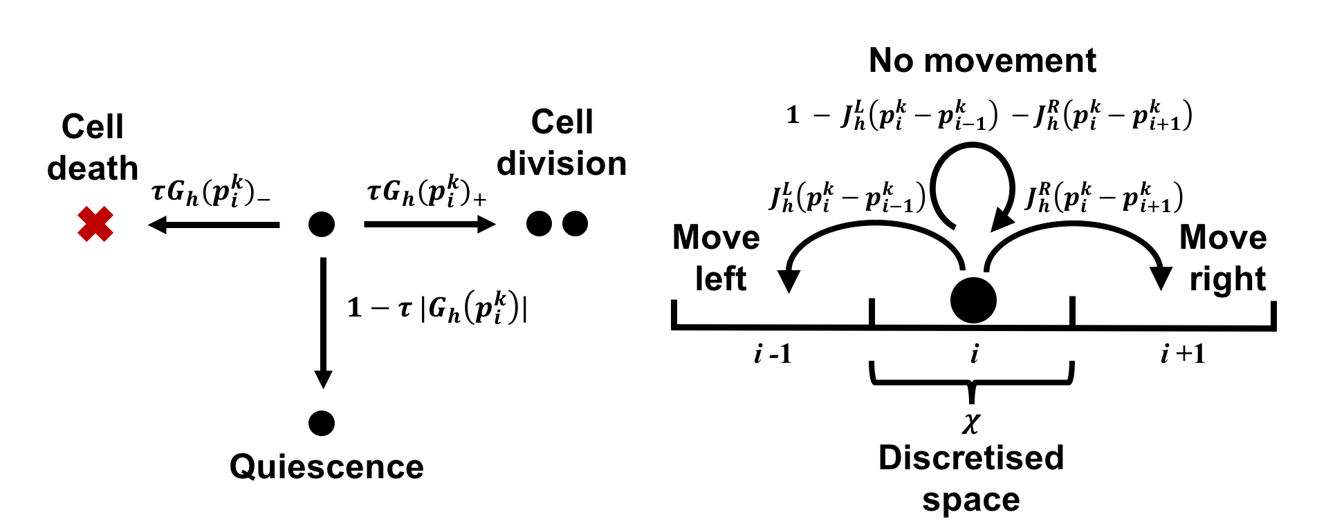 Figure 1
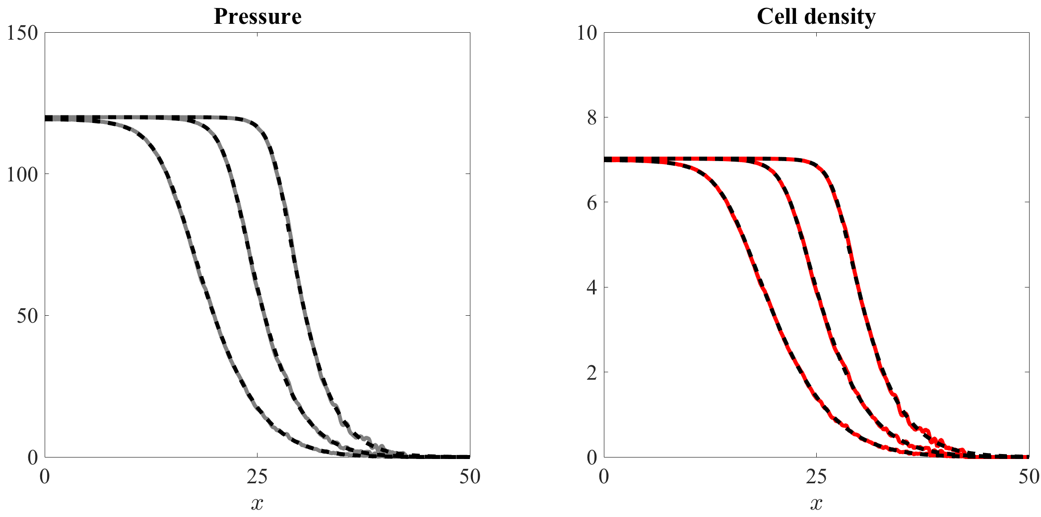 Figure 2
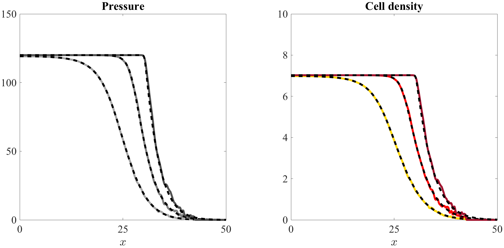 Figure 3
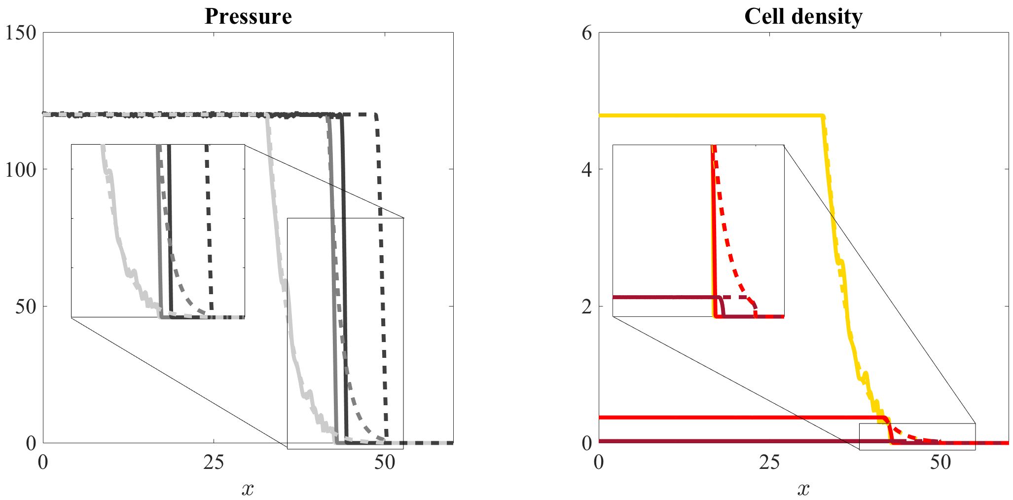 Figure 4
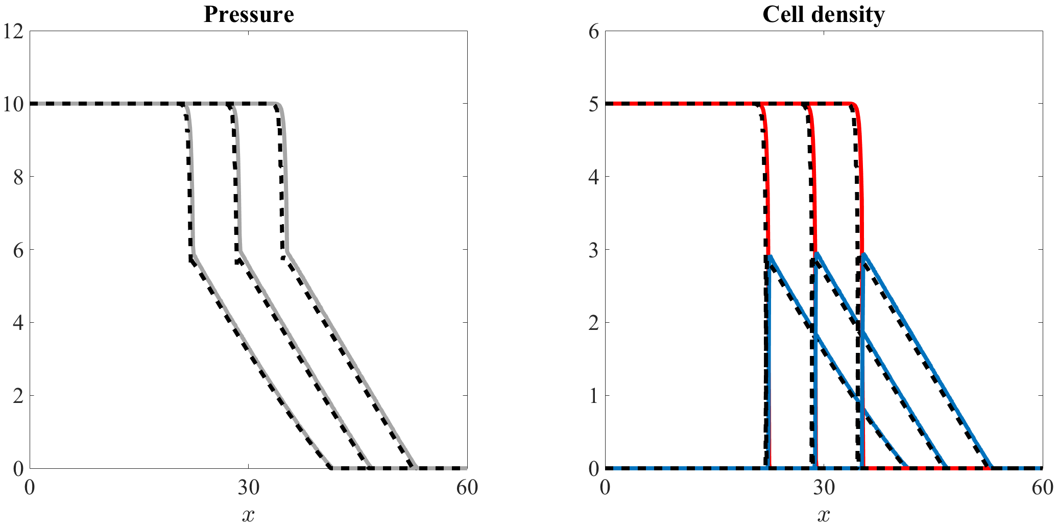 Figure 5
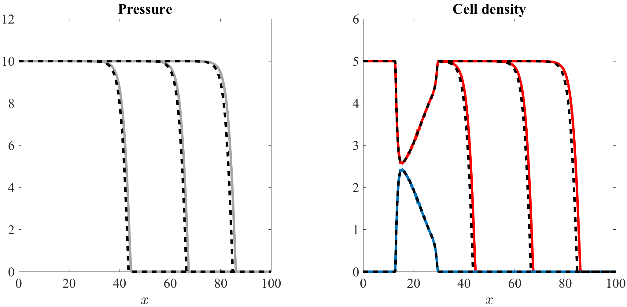 Figure 6
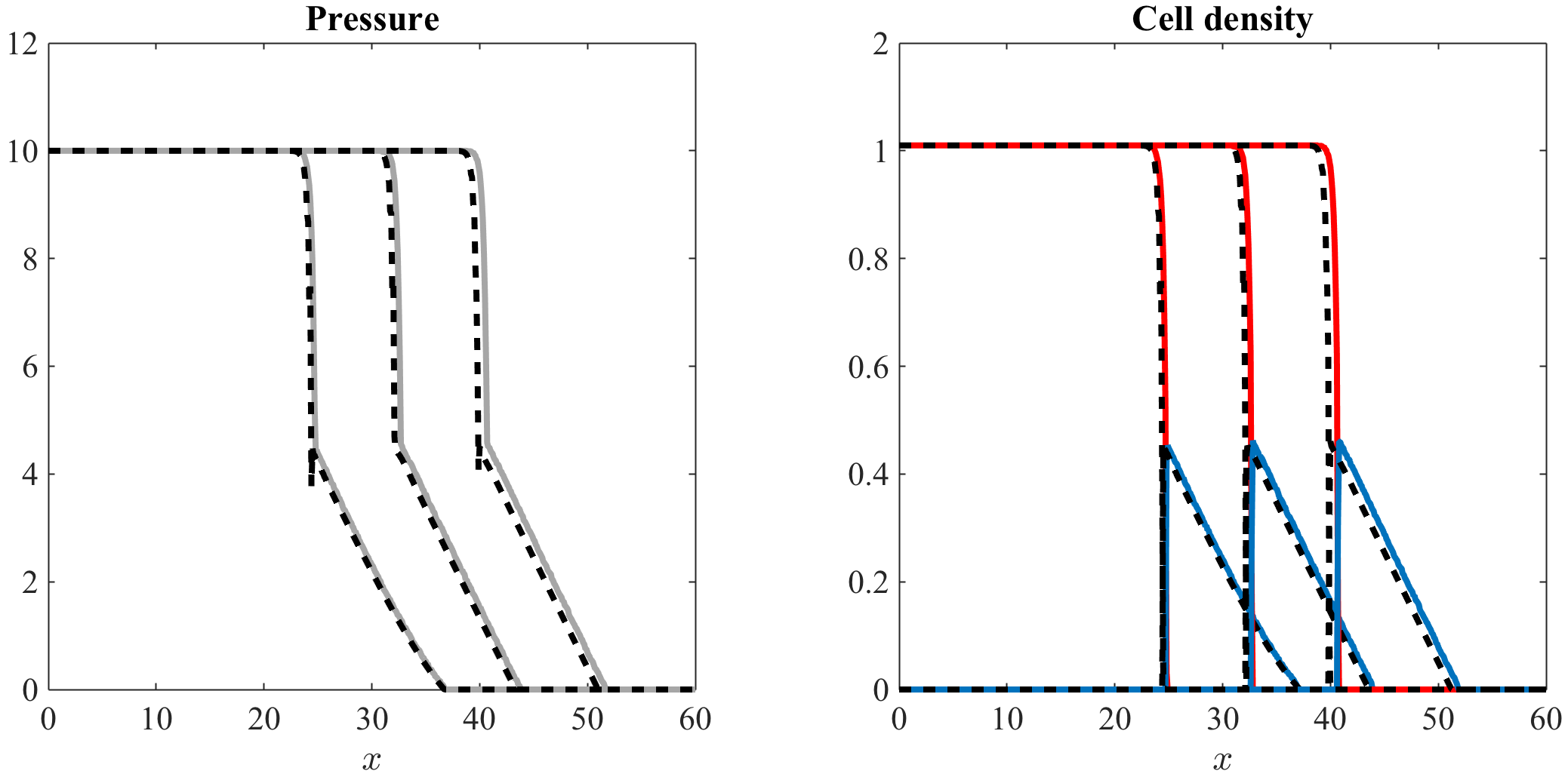 Figure 7
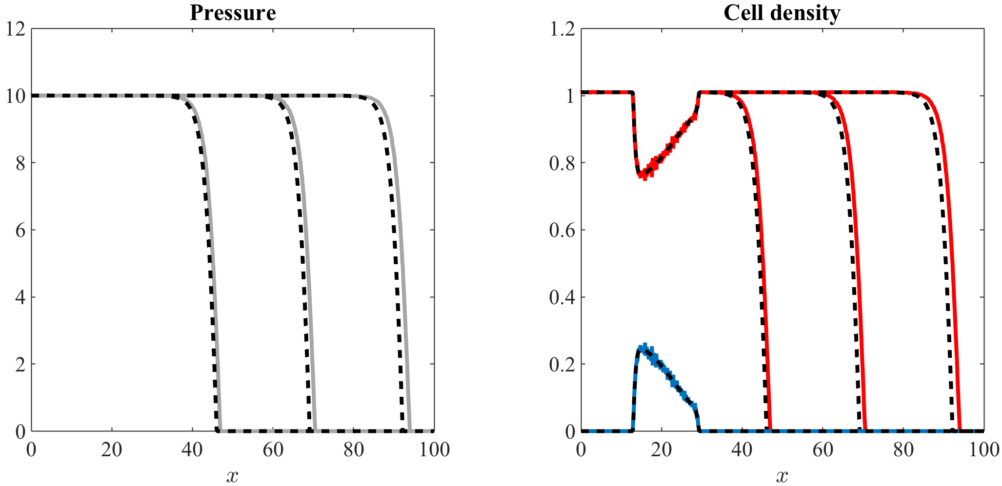 Figure 8
Peer Reviews
No public reviews on file for this paper yet. If you reviewed it on a platform where reviews are public (OpenReview, ICLR, NeurIPS, ICML), you can paste yours below so the community can read it here.
Videos
No videos yet. Explain this paper in a talk, walkthrough, or lecture? Add one.
∎
11institutetext: Mark A J Chaplain 22institutetext: School of Mathematics and Statistics, University of St Andrews, St Andrews, KY16 9SS 22email: [email protected] 33institutetext: Tommaso Lorenzi 44institutetext: School of Mathematics and Statistics, University of St Andrews, St Andrews, KY16 9SS 44email: [email protected] 55institutetext: Fiona R Macfarlane 66institutetext: School of Mathematics and Statistics, University of St Andrews, St Andrews, KY16 9SS
66email: [email protected]
Bridging the gap between individual-based and continuum models of growing cell populations
Mark A J Chaplain
Tommaso Lorenzi
Fiona R Macfarlane
(Received: date / Accepted: date)
Abstract
Continuum models for the spatial dynamics of growing cell populations have been widely used to investigate the mechanisms underpinning tissue development and tumour invasion. These models consist of nonlinear partial differential equations that describe the evolution of cellular densities in response to pressure gradients generated by population growth. Little prior work has explored the relation between such continuum models and related single-cell-based models. We present here a simple stochastic individual-based model for the spatial dynamics of multicellular systems whereby cells undergo pressure-driven movement and pressure-dependent proliferation. We show that nonlinear partial differential equations commonly used to model the spatial dynamics of growing cell populations can be formally derived from the branching random walk that underlies our discrete model. Moreover, we carry out a systematic comparison between the individual-based model and its continuum counterparts, both in the case of one single cell population and in the case of multiple cell populations with different biophysical properties. The outcomes of our comparative study demonstrate that the results of computational simulations of the individual-based model faithfully mirror the qualitative and quantitative properties of the solutions to the corresponding nonlinear partial differential equations. Ultimately, these results illustrate how the simple rules governing the dynamics of single cells in our individual-based model can lead to the emergence of complex spatial patterns of population growth observed in continuum models.
Keywords:
Growing cell populations Pressure-driven cell movement Pressure-limited growth Individual-based models Continuum models
MSC:
92C17 35Q92 92-08 92B05 35C07
1 Introduction
Brief overview of continuum models of growing cell populations.
Continuum models for the spatial dynamics of growing cell populations have been widely used to complement empirical research in developmental biology and cancer research. These models consist of nonlinear partial differential equations that describe the evolution of cellular densities in response to pressure gradients generated by population growth, which can be mechanically regulated, nutrient-limited or pressure-dependent ambrosi2002mechanics ; ambrosi2002closure ; araujo2004history ; bresch2010computational ; byrne2010dissecting ; byrne1995growth ; byrne1996growth ; byrne1997free ; byrne2009individual ; byrne2003two ; byrne2003modelling ; chaplain2006mathematical ; chen2001influence ; ciarletta2011radial ; greenspan1976growth ; lowengrub2009nonlinear ; perthame2014some ; preziosi2003cancer ; ranft2010fluidization ; roose2007mathematical ; sherratt2001new ; ward1999mathematical ; ward1997mathematical .
For a population of cells with growth rate that depends on the local pressure bru2003universal ; byrne2003modelling ; drasdo2012modeling ; ranft2010fluidization , a prototypical example of such models is given by the following equation
[TABLE]
which was proposed by Byrne & Drasdo byrne2009individual . Equation (1) is a conservation equation for the function that represents the density of cells at position , with in the biologically relevant cases, and time . The function stands for the cell pressure and the term is the net growth rate of the cell density.
The second term on the left-hand side of equation (1) represents the rate of change of the cellular density due to pressure-driven cell movement (i.e. the tendency of cells to move towards regions where they feel less compressed). The definition of this term builds on the seminal paper of Greenspan greenspan1976growth and subsequent work of Byrne & Chaplain byrne1997free . In analogy with the classical Darcy’s law for fluids, the parameter can be seen as the cell mobility coefficient, which is defined as the quotient between the permeability of the porous medium in which the cells are embedded (e.g. the extracellular matrix) and the cellular viscosity.
The term on the right-hand side of equation (1) represents the rate of change of the cellular density due to cell proliferation (i.e. cell division and cell death). In the mathematical framework of equation (1), the effect of pressure-limited growth can be captured in a first approximation by assuming the net growth rate to be a smooth function of that satisfies the following assumptions
[TABLE]
In assumptions (2), the parameter stands for the pressure at which cell death exactly compensates cell division. The term homeostatic pressure has been coined to indicate such a critical pressure basan2009homeostatic .
In order to close equation (1) the pressure can be defined according to a barotropic relation . Typically, the function is identically zero for and is monotonically increasing for , with being the density below which cells do not exert any force upon one another tang2014composite . For simplicity, in this paper we let be a smooth function of that satisfies the following assumptions
[TABLE]
For instance, in the attempt to reduce the biological problem to its essentials while ensuring analytical tractability of the mathematical model, Perthame et al. perthame2014hele have proposed the following definition of , which satisfies assumptions (3):
[TABLE]
In definition (4), the parameter provides a measure of the stiffness of the barotropic relation and is a scale factor. The limit corresponds to the case where cells behave like an incompressible fluid. In this asymptotic regime, it has been proven that models of the form of equation (1) converge to free-boundary problems of Hele-Shaw type kim2018porous ; kim2016free ; mellet2017hele ; perthame2014derivation .
The model (1) can be generalised to the case of multiple cell populations with different biophysical properties (i.e. different mobilities and growth rates) as follows
[TABLE]
The system of coupled equations (5) relies on notation and assumptions analogous to those underlying equation (1). In particular, the coefficient represents the mobility of cells in the population and the pressure is defined by a barotropic relation . Here stands for the total cell density, i.e.
[TABLE]
and the function satisfies conditions (3). Moreover, the net growth rate of the cell density can be assumed to be a smooth function of the cell pressure that satisfies assumptions (2) for all .
For example, building on the computational results presented by Drasdo & Hoehme drasdo2012modeling , Lorenzi et al. lorenzi2017interfaces considered the following variant of the system of equations (5)
[TABLE]
complemented with the barotropic relation (4). The system of equations (7) describes the interaction dynamics between a population of proliferating cells (i.e. population ) and a population of nonproliferating cells (i.e. population ) with different mobilities.
Further to the biological and clinical insights into the underpinnings of tissue development and tumour growth they can provide, these continuum models exhibit a range of interesting qualitative behaviours. For instance, it was shown that models in the form of equation (1) admit travelling-wave solutions with composite shapes and discontinuities tang2014composite . Moreover, in analogy with reaction-diffusion systems arising in the mathematical modelling of other biological and ecological problems dancer1999spatial ; mimura2000reaction , models like the system of equations (7) can give rise to sharp interfaces, which bring about spatial segregation between cell populations with different biophysical properties lorenzi2017interfaces .
Derivation of continuum models of growing cell populations from individual-based models.
A key advantage of continuum models for the spatial dynamics of growing cell populations over their individual-based counterparts (i.e. discrete models that track the dynamics of individual cells) drasdo2005coarse ; van2015simulating is that they are amenable to mathematical analysis. This enables a complete exploration of the model parameter space, which ultimately allows more robust conclusions to be drawn. Moreover, compared to individual-based models, continuum models offer the possibility to carry out numerical simulations at the level of larger portions of tissues or even of whole organs, while keeping computational costs within acceptable bounds.
Since continuum models are defined at the scale of whole cell populations, they are usually formulated on the basis of phenomenological considerations, which can hinder a precise mathematical description of crucial biological and physical aspects. On the contrary, stochastic individual-based models that describe the dynamics of single cells in terms of algorithmic rules can be more easily tailored to capture fine details of cellular dynamics, thus making it possible to achieve a more accurate mathematical representation of multicellular systems. Furthermore, individual-based models are able to reproduce the emergence of population-level phenomena that are induced by stochastic fluctuations in single-cell biophysical properties, which are relevant in the regime of low cellular densities and cannot easily be captured by continuum models. Therefore, it is desirable to derive continuum models for the spatial dynamics of cell populations as the appropriate limit of individual-based models for spatial cell movement and proliferation, in order to have a clearer picture of the modelling assumptions that are made and ensure that they correctly reflect the salient features of the underlying application problem.
For this reason, the derivation of continuum models formulated in terms of partial differential equations or partial integrodifferential equations from underlying individual-based models has attracted the attention of a considerable number of mathematicians and physicists. Examples in this active field of research include the derivation of continuum models of chemotaxis from velocity-jump process hillen2009user ; othmer1988models ; othmer2000diffusion ; painter2003modelling or from self-attracting reinforced random walks stevens2000derivation ; stevens1997aggregation ; the derivation of diffusion and nonlinear diffusion equations from underlying random walks champagnat2007invasion ; inoue1991derivation ; oelschlager1989derivation ; othmer2002diffusion ; penington2011building ; penington2014interacting , from systems of discrete equations of motion oelschlager1990large ; murray2009discrete ; murray2012classifying , from discrete lattice-based exclusion processes binder2009exclusion ; dyson2012macroscopic ; fernando2010nonlinear ; johnston2017co ; johnston2012mean ; landman2011myopic ; lushnikov2008macroscopic ; simpson2010cell or from cellular automata deroulers2009modeling ; drasdo2005coarse ; simpson2007simulating ; and, most recently, the derivation of nonlocal models of cell-cell adhesion from position-jump processes buttenschoen2018space . However, with the exception of the results presented in byrne2009individual ; engblom2018scalable ; motsch2018short , little prior work has investigated the relation between single-cell-based models and continuum models in the form of equation (1) and the system of equations (5). In particular, a derivation of these continuum models of growing cell populations from underlying individual-based models of spatial cell movement and proliferation has remained elusive.
Contents of the paper.
In the present paper we aim to bridge such a gap in the existing literature. In Section 2, we develop a simple stochastic individual-based model for the dynamics of growing cell populations. Our model is based on a branching random walk that takes into account the effects of pressure-driven cell movement and pressure-dependent cell proliferation. In Section 3, we show that equation (1) and the system of equations (5) can be formally derived from the branching random walk that underlies our discrete model. In Section 4, we carry out a systematic quantitative comparison between the individual-based model and its continuum counterparts, both in the case of one single cell population and in the case of multiple cell populations with different biophysical properties. In summary, we construct travelling-wave solutions both for equation (1) and for the system of equations (7) (Section 4.1), we present numerical solutions that illustrate the results of the travelling-wave analysis, and we compare such numerical solutions with the results of computational simulations of the individual-based model (Section 4.2). Section 5 concludes the paper and provides a brief overview of possible research perspectives.
2 An individual-based model for growing cell populations
We consider a multicellular system composed of cell populations. We represent each cell within the system as an agent that occupies a position on a lattice. Cells can move and proliferate according to a set of simple rules that result in a discrete-time branching random walk. For ease of presentation, we let cells be arranged along the real line , but there would be no additional difficulty in considering the case of branching random walks in higher spatial dimensions.
We discretise the time variable and the space variable as with and with , respectively, where . We introduce the dependent variable to model the number of cells of population on the lattice site and at the time-step , and we compute the density of cells of population and the total cell density, respectively, as
[TABLE]
Moreover, for each lattice site and time-step we assume the cell pressure to be given by a barotropic relation with being a function of the total cell density that satisfies conditions (3). At each time-step, we allow every cell to undergo pressure-dependent proliferation and pressure-driven movement according to the following algorithmic rules, which are schematised in Figure 1.
Pressure-dependent cell proliferation.
We allow every cell to divide, die or remain quiescent with probabilities that depend on the local pressure, and we assume that a dividing cell is replaced by two identical daughter cells that are placed on the original lattice site of the parent cell. In order to model pressure-limited growth, given the net growth rate that satisfies assumptions (2) for all values of , we assume that at the time-step a focal cell of population on the lattice site can divide with probability
[TABLE]
or die with probability
[TABLE]
or remain quiescent with probability
[TABLE]
We assume the time-step to be sufficiently small so that the quantities (9)-(11) are all between 0 and 1. Under assumptions (2), the definitions (9)-(11) are such that if then every cell on the lattice site can only die or remain quiescent at the time-step. Therefore, we have that
[TABLE]
Pressure-driven cell movement.
We model pressure-driven cell movement (i.e. the tendency of cells to move down pressure gradients) as a biased random walk whereby the movement probabilities depend on the difference between the pressure at the site occupied by a cell and the pressure at the neighbouring sites. In particular, for a focal cell of population on the lattice site at the time-step , we define the probability of moving to the lattice site (i.e. the probability of moving left) as
[TABLE]
where , the probability of moving to the lattice site (i.e. the probability of moving right) as
[TABLE]
where , and the probability of remaining stationary on the lattice site as
[TABLE]
In the above equations, the coefficient is directly proportional to the mobility of cells in population and the parameter is defined in (12). Notice that the definitions (13)-(15) are such that the cells will move down pressure gradients. Moreover, the a priori estimate (12) ensures that the quantities defined according to (13)-(15) are all between 0 and 1.
3 Formal derivation of continuum models
In this section, we show how continuum models of growing cell populations of the form of equation (1) and of the system of equations (5) and (7) can be derived as formal limits of the branching random walk that underlies our stochastic individual-based model.
For a multicellular system the dynamic of which is governed by the algorithmic rules presented in Section 2, the principle of mass balance gives
[TABLE]
and after a little algebra we find
[TABLE]
The above equation simplifies to
[TABLE]
Using the fact that the following relations hold for and sufficiently small
[TABLE]
[TABLE]
[TABLE]
we rewrite equation (16) in the approximate form
[TABLE]
Assuming
[TABLE]
we approximate the terms , and in equation (17) by their second order Taylor expansions about the point . Moreover, since and is a smooth function of , under assumption (18) the pressure is twice continuously differentiable with respect to the variable . Hence we also approximate the terms and in equation (17) by their second order Taylor expansions about the point . In so doing, after a little algebra we find
[TABLE]
which implies
[TABLE]
with
[TABLE]
Dividing both sides of the resulting equation by we obtain
[TABLE]
Letting both and in such a way that
[TABLE]
from (20) we formally obtain the following system of coupled conservation equations
[TABLE]
which can be rewritten as the system of equations (5), that is,
[TABLE]
In a similar way, in the case of one single cell population, letting and dropping the index we formally obtain equation (1). Moreover, we can formally obtain the system of equations (7) by choosing , labelling the two populations by and , and setting and .
Remark 1
We note that condition (21) is a natural counterpart of the usual parabolic scaling of Brownian motion. Hence, our formal derivation does not impose any additional assumptions than those commonly employed for the asymptotic investigation of random walks.
4 Comparison between individual-based and continuum models
In this section, we carry out a systematic quantitative comparison between the outcomes of our individual-based model, both in the case of one cell population and in the case of two cell populations, and the solutions of the corresponding continuum models. We first establish the existence of travelling-wave solutions for the continuum models (1) and (7) (Section 4.1). We then construct numerical solutions of the model equations which illustrate the results of the travelling-wave analysis and we compare such numerical solutions with the results of computational simulations of our individual-based model (Section 4.2).
4.1 Travelling-wave analysis of the continuum models
We first consider the continuum model (1) and we look for one-dimensional travelling-wave solutions of the form
[TABLE]
that satisfy the following asymptotic conditions
[TABLE]
Therefore, we study the existence of pairs that satisfy the problem defined by the differential equation
[TABLE]
subject to conditions (23). Our main results are summarised by the following theorem.
Theorem 4.1
Under assumptions (2) and (3), there exists such that the travelling-wave problem defined by the differential equation (24) subject to conditions (23) admits a nonnegative and nonincreasing solution .
Proof
We divide the proof of Theorem 4.1 into two steps. First we prove that for fixed the differential equation (24) subject to the asymptotic conditions (23) admits a nonnegative and nonincreasing solution (Step 1). Then we show that there exists a unique value of the wave speed that satisfies the travelling-wave problem (Step 2).
Step 1. Multiplying both sides of the differential equation (24) by we obtain the following boundary-value problem for
[TABLE]
[TABLE]
Let be a critical point of in . Using the differential equation (25) we see that
[TABLE]
and, under assumptions (2) and conditions (26), using the strong maximum principle we conclude that in and that cannot have a local minimum in , i.e.
[TABLE]
Hence the solution of the differential equation (25) subject to conditions (26) is a nonnegative and nonincreasing function that satisfies
[TABLE]
Since and is a smooth monotonically increasing function of , we can then conclude that the cell density is a nonnegative and nonincreasing function as well.
Step 2. Using a method similar to that used in Step 5 of the proof of Theorem 4.2 one can prove that is a monotonically decreasing function of the parameter . This ensures that given the pressure or, equivalently, the cell density the wave speed can be uniquely identified through a monotonicity argument. ∎
We then turn to the travelling-wave analysis of the system of equations (7). On the basis of the results presented in lorenzi2017interfaces , we consider one-dimensional travelling-wave solutions of the form
[TABLE]
that satisfy the following conditions
[TABLE]
for some , along with the asymptotic condition
[TABLE]
Hence, we study the existence of triples along with that satisfy the problem defined by the following system of differential equations
[TABLE]
subject to conditions (29) and (30). Notice that the principle of mass conservation gives
[TABLE]
for some that represents the number of cells in population . Our main results are summarised by the following theorem.
Theorem 4.2
Under assumptions (2) and (3), for any given, there exists and such that the system of differential equations (31) subject to conditions (29) and (30) admits a component-wise nonnegative solution with nonincreasing, and nonincreasing and satisfying condition (32). Moreover, the pressure has a kink in with
[TABLE]
Proof
Building upon the method of proof presented by Lorenzi et al lorenzi2017interfaces for the case of the barotropic relation (4), we prove Theorem 4.2 in five steps. We fix the parameter and first prove that, for given, the problem under study admits a component-wise nonnegative solution with nonincreasing and with the value of being determined by condition (32) (Step 1), and with nonincreasing (Step 2). Then we prove that the total cell density is continuous on (Step 3) and the jump condition (33) holds (Step 4). Finally, we show that there exists a unique value of the wave speed that satisfies the travelling-wave problem (Step 5).
Step 1. Integrating the differential equation (31)2 between a generic point and , and using the fact that both and as , we find
[TABLE]
Integrating equation (34) between a generic point and , and using the fact that , gives
[TABLE]
which implies that
[TABLE]
Since on , under assumptions (3), we have that is a monotonically decreasing function of in . Hence, the results (34) and (35) allow us to conclude that is decreasing in . Moreover, for given, since the value of is uniquely determined for all , the value of is uniquely fixed by the mass conservation condition (32).
Step 2. Since on and, therefore, on , multiplying both sides of the differential equation (31)1 by we obtain the following boundary-value problem for
[TABLE]
[TABLE]
Hence, using a method similar to that used in Step 1 of the proof of Theorem 4.1 one can prove that is decreasing in .
Step 3. The results proved in Step 1 and Step 2 ensure that the total cell density is nonincreasing and continuous in and in . We now prove that is continuous in . Adding together the differential equations (31)1 and (31)2 gives
[TABLE]
Multiplying both sides of the above differential equation by and using the fact that
[TABLE]
we find that
[TABLE]
Integrating both sides of the latter differential equation between a generic point and , and estimating the right-hand side from above by using the fact that for all , and , yields
[TABLE]
The above integral inequality ensures that . This result along with the fact that allow us to conclude that is continuous in . Since and is a smooth monotonically increasing function of , we have that the total cell density is continuous in as well.
Step 4. Integrating the differential equation (39) between a generic point and and using the fact that yields
[TABLE]
Letting and using the fact that and on we find that
[TABLE]
Similarly, letting and using the fact that and on gives
[TABLE]
Since is continuous in , combining equations (40) and (41) we obtain
[TABLE]
This result along with the expression (34) for gives
[TABLE]
From the latter equation we deduce the jump condition (33). Moreover, substituting the expression of into the differential equation (37) gives .
Step 5. We prove that is a monotonically decreasing function of the parameter on . This ensures that given the cell density the wave speed can be uniquely identified through a monotonicity argument. Recalling that on and, therefore, on , differentiating equation (31)1 with respect to we find
[TABLE]
with
[TABLE]
On the other hand, differentiating equation (31)1 with respect to gives
[TABLE]
with
[TABLE]
Using the fact that , we rewrite the differential equations (42) and (43), respectively, as
[TABLE]
and
[TABLE]
Since , we have
[TABLE]
Hence, introducing the notation , and
[TABLE]
we rewrite the differential equations (44) and (45), respectively, as
[TABLE]
with
[TABLE]
and
[TABLE]
with
[TABLE]
Since for all and , noting that both and as and the right-hand side of the differential equation (48) contains the additional term compared to the right-hand side of the differential equation (46), we deduce that , which concludes the proof of Theorem 4.2. ∎
Remark 2
Based on the jump condition (33), we expect the travelling-wave solution of Theorem 4.2 to be unstable if . In fact, a small perturbation of that is greater than zero on will propagate with approximate speed . Noting that when the jump condition (33) gives , we deduce that such a perturbation will separate from the rest of the travelling wave .
4.2 Quantitative comparison between individual-based and continuum models
4.2.1 One cell population
We begin by comparing the computational simulation results of our individual-based model in the case of one cell population with the numerical solutions of equation (1). For consistency with equation (1), we set and we drop the index both from the functions and from the parameters of the individual-based model. A complete description of the setup of numerical simulations is given in Appendix A.1 and Appendix B.1. In particular, we use the following definition of the net growth rate
[TABLE]
so that assumptions (2) are satisfied.
Travelling fronts.
Figure 2, along with the video accompanying it (vid. Online Resource 1), demonstrates that there is an excellent quantitative match between the numerical solutions of equation (1) and the computational simulation results of our individual-based model. In agreement with the results established by Theorem 4.1, the cell density is nonincreasing and connects the homogeneous steady state to the homogeneous steady state . Accordingly, the cell pressure is nonincreasing and connects the homogeneous steady state to the homogeneous steady state .
Higher values of lead to higher speed of invasion.
Figure 3, along with the video accompanying it (vid. Online Resource 2), indicates that, as one would expect, increasing the value of the parameter in the definition (50) of accelerates the growth of the cell population, thus leading to a higher speed of invasion.
Differences between the outcomes of individual-based and continuum models in the presence of sharp transitions from high to low cell densities.
The results presented so far indicate that there is an excellent agreement between the computational simulation results of our individual-based model and the solutions of the corresponding continuum models. However, due to extinction phenomena related to stochasticity effect that occur in the individual-based model for low cell densities, we expect differences between the outcomes of the two modelling approaches to emerge in the presence of sharp transitions from high to low total cell densities. In order to verify this hypothesis, exploiting the asymptotic results of Perthame et al. perthame2014hele – who have shown that under the barotropic relation (4) sufficiently high values of the parameter lead equation (1) to develop sharper invasion fronts – we compare the computational simulation results of our individual-based model in the case of one cell population with the numerical solutions of equation (1) under the barotropic relation (4) for increasing values of . A complete description of the setup of numerical simulations is given in Appendix A.1 and Appendix B.1. The results obtained are summarised by Figure 4 which shows that larger values of the parameter can bring about sharper invasion fronts, which come along with more abrupt variations in the cell density, thus leading to more evident differences between the computational simulation results of the stochastic individual-based model and the numerical solutions of equation (1) at the front of invasion. Ultimately, this causes the invasion front of the individual-based model to travel at the same speed but behind the front of the corresponding continuum model.
4.2.2 Two cell populations
We now turn to the case of two cell populations and we compare computational simulation results of our individual-based model with numerical solutions of the system of equations (7). For consistency with the system of equations (7), we choose , and we set and in the individual-based model. Full details of the setup of numerical simulations can be found in Appendix A.2 and Appendix B.2 for the results reported in Figures 5 and 6, and Appendix A.3 and Appendix B.3 for the results reported in Figures 7 and 8. In particular, we use the definition (50) of the net growth rate with the homeostatic pressure and we let the population of nonproliferating cells (i.e. population ) be ahead of the population of proliferating cells (i.e. population ) at the initial time .
Figures 5 and 6, along with the videos accompanying them (vid. Online Resource 3 and Online Resource 4), demonstrate that there is an excellent quantitative match between the numerical solutions of the system of equations (7) and the computational simulation results of our individual-based model, both in the case where and when . Over time, the pressure converges to the homeostatic pressure while the cell density converges to the corresponding value .
Travelling fronts and spatial segregation between the two cell populations.
If (i.e. if ), in agreement with the results established by Theorem 4.2, spatial segregation occurs and the two cell populations remain separated by a sharp interface (vid. Figure 5 and Online Resource 3). The population of nonproliferating cells stays ahead of the population of proliferating cells and, over the regions where they are greater than zero, the cell densities are nonincreasing. The pressure itself is continuous across the interface between the two cell populations, whereas its first derivative jumps from a lower negative value to a larger negative value, i.e. the sign of the jump coincides with (cf. the jump condition (33)).
Mixing between the two cell populations.
If (i.e. if ) the cell population 2 is left behind by the cell population 1, which ultimately propagates alone (vid. Figure 6 and Online Resource 4). This is consistent with the heuristic argument provided in Remark 2, which suggests that the travelling-wave solutions of Theorem 4.2 are unstable in the case where .
Numerical simulations for more realistic barotropic relations.
In this paper, we have focused on barotropic relations that satisfy assumptions (3). However, as mentioned earlier in Section 1, more realistic barotropic relations satisfy the following conditions
[TABLE]
with . Figures 7 and 8, along with the videos accompanying them (vid. Online Resource 5 and Online Resource 6), display the computational simulation results of our stochastic individual-based model and the numerical solutions of the system of equations (7) obtained under a barotropic relation that satisfies the more general assumptions (51) (vid. Appendix A.3 and Appendix B.3 for a complete description of the numerical simulation setup). These computational results and numerical solutions clearly share the same properties as those of Figures 5 and 6. This supports the conclusion that the essentials of the results obtained using barotropic relations of the form (3) remain intact even under the more realistic assumptions (51).
5 Conclusions and research perspectives
In summary, we have developed a simple, yet effective, stochastic individual-based model for the spatial dynamics of multicellular systems whereby cells undergo pressure-driven movement and pressure-dependent proliferation. We have shown that nonlinear partial differential equations commonly used to model the spatial dynamics of growing cell populations can be formally derived from the branching random walk that underlies our discrete model. Moreover, we have carried out a systematic comparison between the individual-based model and its continuum counterparts, both in the case of one single cell population and in the case of multiple cell populations with different biophysical properties. The outcomes of our comparative study demonstrate that the results of computational simulations of the individual-based model faithfully mirror the qualitative and quantitative properties of the solutions to the corresponding nonlinear partial differential equations. Ultimately, these results illustrate how the simple rules governing the dynamics of single cells in our individual-based model can lead to the emergence of complex spatial patterns of population growth observed in continuum models – e.g. travelling waves with composite shapes and sharp interfaces corresponding to spatial segregation between cell populations with different biophysical properties.
We have focussed on the case of one spatial dimension and considered barotropic relations that satisfy assumptions (3). However, the model presented here, as well as the related formal method to derive corresponding continuum models, can be adapted to higher spatial dimensions and more realistic barotropic relations of the form (51). In this regard, it would be interesting to use our stochastic individual-based model to further investigate the formation of finger-like patterns of invasion observed for the system of equations (7) posed on a two dimensional spatial domain lorenzi2017interfaces . Such spatial patterns resemble infiltrating patterns of cancer-cell invasion commonly observed in breast tumours wang2012adipose . An additional development of our study would be to compare the results presented here with those obtained from equivalent models defined on irregular lattices, as well as to investigate how our modelling approach could be related to off-lattice models of growing cell populations drasdo2005coarse ; motsch2018short ; van2015simulating .
Our modelling framework can be easily extended to incorporate additional layers of biological complexity, such as nutrient-limited proliferation, undirected random cell movement, chemotaxis and haptotaxis. These are all lines of research that we will be pursuing in the near future.
Appendix A Details of numerical simulations of the individual-based model
We use a uniform discretisation of the interval that consists of 1001 points as the spatial domain (i.e. the grid-step is ) and we choose the time-step . We implement zero-flux boundary conditions by letting the attempted move of a cell be aborted if it requires moving out of the spatial domain. For all simulations, we use the definition (50) of and we perform numerical computations in Matlab. Further details specific either to the case of one single cell population or to the case of two cell populations are provided in the next subsections.
A.1 Setup of numerical simulations for the case of one single cell population
For consistency with equation (1), we set and we drop the index both from the functions and from the parameters of the individual-based model. We define the rate in equations (9)-(11) according to equation (50). We set the homeostatic pressure for the simulation results reported in Figure 2 and Figure 3, while we choose for the simulation results of Figure 4. Moreover, we choose for the simulation results reported in Figure 2, for the simulation results of Figure 4, and for the simulation results of Figure 3. We set in equations (13)-(15) and we define the pressure according to the following barotropic relation
[TABLE]
which satisfies conditions (3). We let for the simulation results of Figure 4, while we choose for the simulation results reported in Figure 2 and Figure 3. We use the initial cell density
[TABLE]
The results presented in Figure 2 and Figure 3 correspond to the average over three simulations of our individual-based model, while the results in Figure 4 correspond to one single simulation when or and the average over two simulations when .
A.2 Setup of numerical simulations for the case of two cell populations – Figure 5 and Figure 6
For consistency with the system of equations (7), we choose , and we set and in equations (9)-(11), where is defined according to equation (50) with the homeostatic pressure and the factor . We set and in equations (13)-(15) for the simulation results reported in Figure 5, while we consider and for the simulation results of Figure 6. We define the pressure according to the following simplified barotropic relation
[TABLE]
which satisfies conditions (3). We make use of the initial cell densities
[TABLE]
where
[TABLE]
The results presented in Figure 5 and Figure 6 correspond to one single simulation of our individual-based model.
A.3 Setup of numerical simulations for the case of two populations – Figure 7 and Figure 8
For consistency with the system of equations (7), we choose , and we set and in equations (9)-(11), where is defined according to equation (50) with the homeostatic pressure and the factor . We set and in equations (13)-(15) for the simulation results reported in Figure 7, while we consider and for the simulation results of Figure 8. We define the pressure according to the following barotropic relation
[TABLE]
which satisfies conditions (51). We make use of the initial cell densities (52) with
[TABLE]
The results presented in Figure 7 and Figure 8 correspond to one single simulation of our individual-based model.
Appendix B Details of numerical simulations of the continuum models
We let and we construct numerical solutions for equation (1) and for the system of equations (7) complemented with zero Neumann boundary conditions. We use a finite volume method based on a time-splitting between the conservative and nonconservative parts. For the conservative parts, transport terms are approximated through an upwind scheme whereby the cell edge states are calculated by means of a high-order extrapolation procedure leveque2002finite , while the forward Euler method is used to approximate the nonconservative parts. We consider a uniform discretisation of the interval that consists of 1001 points and we perform numerical computations in Matlab. For all simulations, we use the definition (50) of . Further details specific either to the case of one cell population or to the case of two cell populations are provided in the next subsections.
B.1 Setup of numerical simulations for equation (1)
The rate is defined according to equation (50) with the homeostatic pressure for the numerical solutions reported in Figure 2 and Figure 3, while we choose for the numerical solutions of Figure 4. Moreover, we choose for the numerical solutions reported in Figure 2, for the numerical solutions of Figure 4, and for the numerical solutions reported in Figure 3. We define the pressure according to the following barotropic relation
[TABLE]
which satisfies conditions (3). We let for the numerical solutions of Figure 4, while we choose for the numerical solutions reported in Figure 2 and Figure 3. Given the parameter values used for the individual-based model in the case of one single cell population, we choose the mobility for the numerical solutions reported in Figure 2 and Figure 3, while we set for the numerical solutions of Figure 4. In this way, both values of satisfy condition (21) for . We impose the initial condition
[TABLE]
B.2 Setup of numerical simulations for the system of equations (7) – Figure 5 and Figure 6
The rate is defined according to equation (50) with the homeostatic pressure and . Given the parameter values used for the individual-based model in the case of two cell populations, we choose the mobilities and for the numerical solutions reported in Figure 5, and the mobilities and for the numerical solutions of Figure 6. This ensures that conditions (21) for are satisfied. We define the pressure according to the following simplified barotropic relation
[TABLE]
which satisfies conditions (3). We impose the initial conditions
[TABLE]
where
[TABLE]
B.3 Setup of numerical simulations for the system of equations (7) – Figure 7 and Figure 8
The rate is defined according to equation (50) with the homeostatic pressure and . Given the parameter values used for the individual-based model in the case of two cell populations, we choose the mobilities and for the numerical solutions reported in Figure 7, and the mobilities and for the numerical solutions of Figure 8. This ensures that conditions (21) for are satisfied. We define the pressure according to the following barotropic relation
[TABLE]
which satisfies conditions (51). We impose the initial conditions (53) with
[TABLE]
Acknowledgements.
FRM is funded by the Engineering and Physical Sciences Research Council (EPSRC). TL and FRM gratefully acknowledge Dirk Drasdo and Luís Neves de Almeida for insightful discussions.
The reference list from the paper itself. Each links out to its DOI / PubMed record.
- 1(1) Ambrosi, D., Mollica, F.: On the mechanics of a growing tumor. Int. J. Eng. Sci. 40 (12), 1297–1316 (2002)
- 2(2) Ambrosi, D., Preziosi, L.: On the closure of mass balance models for tumor growth. Math. Mod. Meth. Appl. Sci. 12 (05), 737–754 (2002)
- 3(3) Araujo, R.P., Mc Elwain, D.S.: A history of the study of solid tumour growth: The contribution of mathematical modelling. Bull. Math. Biol. 66 (5), 1039–1091 (2004)
- 4(4) Basan, M., Risler, T., Joanny, J.F., Sastre-Garau, X., Prost, J.: Homeostatic competition drives tumor growth and metastasis nucleation. HFSP Journal 3 (4), 265–272 (2009)
- 5(5) Binder, B.J., Landman, K.A.: Exclusion processes on a growing domain. J. Theor. Biol. 259 (3), 541–551 (2009)
- 6(6) Bresch, D., Colin, T., Grenier, E., Ribba, B., Saut, O.: Computational modeling of solid tumor growth: The avascular stage. SIAM J. Sci. Comput. 32 (4), 2321–2344 (2010)
- 7(7) Brú, A., Albertos, S., Subiza, J.L., García-Asenjo, J.L., Brú, I.: The universal dynamics of tumor growth. Biophys. J. 85 (5), 2948–2961 (2003)
- 8(8) Buttenschoen, A., Hillen, T., Gerisch, A., Painter, K.J.: A space-jump derivation for non-local models of cell–cell adhesion and non-local chemotaxis. J. Math. Biol. 76 (1-2), 429–456 (2018)