This paper explores the exponents associated with $Y$-systems of finite type Dynkin diagrams, proposing a conjectural formula linked to root systems and $q$-series, with proofs for specific cases and implications for affine Lie algebra modules.
Contribution
It introduces a conjectural formula relating $Y$-system exponents to root systems, proves it for certain cases, and connects these exponents to $q$-series identities and affine Lie algebra modules.
Findings
01
Conjectural formula for exponents in $Y$-systems based on root systems.
02
Proof of the conjecture for $(A_1, \, \ell)$ and $(A_r, 2)$ cases.
03
Relationship established between exponents and asymptotic dimensions of affine Lie algebra modules.
Abstract
Let Xr be a finite type Dynkin diagram, and ℓ be a positive integer greater than or equal to two. The Y-system of type Xr with level ℓ is a system of algebraic relations, whose solutions have been proved to have periodicity. For any pair (Xr,ℓ), we define an integer sequence called exponents using formulation of the Y-system by cluster algebras. We give a conjectural formula expressing the exponents by the root system of type Xr, and prove this conjecture for (A1,ℓ) and (Ar,2) cases. We point out that a specialization of this conjecture gives a relationship between the exponents and the asymptotic dimension of an integrable highest weight module of an affine Lie algebra. We also give a point of view from q-series identities for this relationship.
Figures4
Click any figure to enlarge with its caption.
Figure 5
Figure 5
Figure 6
Figure 6
Equations501
t(ℓ+h∨)μ∘μ∘⋯∘μ(y)=y,
t(ℓ+h∨)μ∘μ∘⋯∘μ(y)=y,
t=⎩⎨⎧123if Xr=Ar,Dr,E6,E7 or E8,if Xr=Br,Cr or F4,if Xr=G2,
t=⎩⎨⎧123if Xr=Ar,Dr,E6,E7 or E8,if Xr=Br,Cr or F4,if Xr=G2,
Bij=⎩⎨⎧−BijBij+BikBkjBij−BikBkjBijif i=k or j=k,if Bik>0 and Bkj>0,if Bik<0 and Bkj<0,otherwise,
Bij=⎩⎨⎧−BijBij+BikBkjBij−BikBkjBijif i=k or j=k,if Bik>0 and Bkj>0,if Bik<0 and Bkj<0,otherwise,
Q(0)μm1Q(1)μm2⋯μmTQ(T)νν(Q(T)).
Q(0)μm1Q(1)μm2⋯μmTQ(T)νν(Q(T)).
\displaystyle\mathcal{F}_{\mathrm{sf}}=\left\{\frac{f(y_{1},\dots,y_{n})}{g(y_{1},\dots,y_{n})}\in\mathcal{F}\,\bigg{|}\,\begin{array}[]{l}\text{$f$ and $g$ are non-zero polynomials in $\mathbb{Q}[y_{1},\dots,y_{n}]$}\\
\text{with non-negative coefficients}\end{array}\right\}
\displaystyle\mathcal{F}_{\mathrm{sf}}=\left\{\frac{f(y_{1},\dots,y_{n})}{g(y_{1},\dots,y_{n})}\in\mathcal{F}\,\bigg{|}\,\begin{array}[]{l}\text{$f$ and $g$ are non-zero polynomials in $\mathbb{Q}[y_{1},\dots,y_{n}]$}\\
\text{with non-negative coefficients}\end{array}\right\}
Bij=⎩⎨⎧−Cijδi′j′Cijδi′j′−δijCi′j′δijCi′j′0if i:(−+), j:(++) or i:(+−), j:(−−),if i:(++), j:(−+) or i:(−−), j:(+−),if i:(++), j:(+−) or i:(−−), j:(−+),if i:(+−), j:(++) or i:(−+), j:(−−),otherwise.
Bij=⎩⎨⎧−Cijδi′j′Cijδi′j′−δijCi′j′δijCi′j′0if i:(−+), j:(++) or i:(+−), j:(−−),if i:(++), j:(−+) or i:(−−), j:(+−),if i:(++), j:(+−) or i:(−−), j:(−+),if i:(+−), j:(++) or i:(−+), j:(−−),otherwise.
Peer Reviews
No public reviews on file for this paper yet. If you reviewed it on a platform where reviews are public (OpenReview, ICLR, NeurIPS, ICML), you can paste yours below so the community can read it here.
Videos
No videos yet. Explain this paper in a talk, walkthrough, or lecture? Add one.
Full text
\FirstPageHeading
\ShortArticleName
Exponents Associated with Y-Systems and their Relationship with q-Series
Department of Mathematical and Computing Science, Tokyo Institute of Technology,
2-12-1 Ookayama, Meguro-ku, Tokyo 152-8550, Japan
\Email[email protected]
\ArticleDates
Received September 27, 2019, in final form April 02, 2020; Published online April 18, 2020
\Abstract
Let Xr be a finite type Dynkin diagram, and ℓ be a positive integer greater than or equal to two. The Y-system of type Xr with level ℓ is a system of algebraic relations, whose solutions have been proved to have periodicity. For any pair (Xr,ℓ), we define an integer sequence called exponents using formulation of the Y-system by cluster algebras. We give a conjectural formula expressing the exponents by the root system of type Xr, and prove this conjecture for (A1,ℓ) and (Ar,2) cases. We point out that a specialization of this conjecture gives a relationship between the exponents and the asymptotic dimension of an integrable highest weight module of an affine Lie algebra. We also give a point of view from q-series identities for this relationship.
In the study of thermodynamic Bethe ansatz, Zamolodchikov introduced a system of algebraic relations called Y-system for any finite type simply laced Dynkin diagram and conjectured that solutions of the Y-system have periodicity. This periodicity conjecture was proved by Fomin and Zelevinsky [5]. Their proof was implicitly based on the theory of cluster algebras that they introduced in [4].
In fact, in [6] they refined the result on the periodicity using the concept in cluster algebras called Y-seed mutations.
More generally, for any finite type Dynkin diagram Xr (=Ar, Br, Cr, Dr, E6,7,8, F4 or G2) and integer ℓ≥2 called level,
the Y-system associated with the pair (Xr,ℓ) is defined in [21].
When X is ADE and the level is 2, this is the Y-system introduced by Zamolodchikov.
The periodicities for these Y-systems were also proved in [12, 13, 18].
Their proof used the quiver representation theory, in particular the algebraic objects called the cluster categories.
Although these periodicities are themselves very interesting,
it is also interesting that they relate to conformal field theories through the Rogers dilogarithm function.
The sum of special values of the Rogers dilogarithm function associated with the Y-system gives the central charge of a conformal field theory [12, 13, 29].
This is called the dilogarithm identities in conformal field theories.
Note that the central charge also appears as the exponential growth of a character in the representation theory of affine Lie algebras [15].
For the proof of these identities, the periodicity of the Y-system mentioned earlier plays an essential role.
The purpose of this paper is to introduce a sequence of integers associated with the Y-system that we call exponents and to reveal interesting features of it.
In particular, we give a conjectural formula on the exponents that gives a new connection between the theory of cluster algebras and the representational theory of affine Lie algebras, and give proofs for some cases.
In order to define the exponents, we first review roughly formulation of the Y-systems by cluster algebras.
First, we define a quiver Q(Xr,ℓ) for a pair (Xr,ℓ).
Then, we can obtain the Y-system as algebraic relations between rational functions obtained by repeating mutations, which are certain operations defined on quivers.
In particular, we can paraphrase the periodicity of the Y-system associated with a pair (Xr,ℓ) to the periodicity of the cluster transformation μ, which is a rational function obtained from a mutation sequence on Q(Xr,ℓ).
Let I be the set of vertices in Q(Xr,ℓ).
Then the cluster transformation μ is actually an I-tuple of single rational functions in the variables y:=(yi∣i∈I),
that is, μ∈Q(yi∣i∈I)I.
Keller [18] (for X=ADE) and Inoue et al. [12, 13] (for X=BCFG) proved the periodicity of the Y-system by showing that μ has the following periodicity:
[TABLE]
where t is defined by
[TABLE]
and h∨ is the dual Coxeter number of Xr.
Using this result, we define the exponents as follows. First, we see that there is a unique η∈(R>0)I that satisfies μ(η)=η.
Then, let J(y) be the Jacobian matrix of the rational function μ:
[TABLE]
The periodicity of μ implies that the t\big{(}\ell+h^{\vee}\big{)}-th power of J(η) is the identity matrix.
Thus all the eigenvalues of J(η) are t\big{(}\ell+h^{\vee}\big{)}-th root of unities.
These eigenvalues can be written as
[TABLE]
using a sequence of integers 0\leq m_{1}\leq m_{2}\leq\dots\leq m_{\lvert\mathbf{I}\rvert}<t\big{(}\ell+h^{\vee}\big{)}. We say that this sequence m1,…,m∣I∣ is the exponents of Q(Xr,ℓ).
We give a conjectural formula on the exponents in terms of root systems.
Let Δ be the root system of type Xr with an inner product (⋅∣⋅) normalized as (α∣α)=2 for long roots α.
Let α1,…,αr be simple roots of Δ.
For any a=1,…,r, we define an integer ta by ta=2/(αa∣αa).
Let Δlong and Δlong be the set of the long roots and the short roots, respectively.
Let ρ be the half of the sum of the positive roots.
Using these materials, we define two polynomials NXr,ℓ(x) and DXr,ℓ(x) by
[TABLE]
where the polynomials DXr,ℓlong(x) and DXr,ℓshort(x) are defined by
[TABLE]
The following formula is the main conjecture of this paper.
It says that the exponents are obtained from the ratio of NXr,ℓ(x) and DXr,ℓ(x).
Conjecture 1.1**.**
The following identity holds for the characteristic polynomial of J(η):
[TABLE]
We prove the conjecture in the following cases. In these cases, we give explicit expressions for eigenvectors of J(η) using known explicit expressions for η.
This conjecture gives a relationship between cluster algebras and root systems.
Even more interestingly, it relates to the representation theory of affine Lie algebras.
Let us explain this.
Let g be the finite dimensional simple Lie algebra of type Xr,
and g^ be the affine Lie algebra associated with g.
It is a central extension of the loop algebra of g together with a derivation operator d.
Let L(Λ) be the integrable highest weight g^-module with the highest weight Λ.
The (specialized) character χΛ(q) is a q-series such that its coefficients are the multiplicities of the eigenvalues of the derivation operator d in L(Λ).
If we set q=e2πiτ, the character χΛ(q) converges to a holomorphic function
on the upper half-plane H={τ∈C∣Imτ>0}.
Let τ↓0 denote the limit in the positive imaginary axis.
Kac and Peterson [15] found that χΛ(q) has the following asymptotics:
[TABLE]
for some rational number c and real number a(Λ).
The real number a(Λ) is called the asymptotic dimension of L(Λ).
They also found the explicit formula of asymptotic dimensions.
Using their formula, we find that the right-hand side of our conjecture at x=1 and the asymptotic dimension
of L(ℓΛ0) where Λ0 is the [math]-th fundamental weight is related as follows:
[TABLE]
where P and Q are the weight lattice and the root lattice for g, respectively.
Therefore, if the conjecture is true, we can describe the asymptotic dimension using the exponents.
Another interesting feature about the exponents that we deal with in this paper is that the relationship between the exponents and partition q-series.
Partition q-series, which is defined by Kato and Terashima [17], is a certain q-series associated with a mutation sequence.
Typically, it has the following form:
[TABLE]
where T is a positive integer, K is a T×T positive definite symmetric matrix with rational coefficients, and (q)n is defined by
[TABLE]
This type of q-series has been studied in various contexts, such as characters of conformal field theories, Rogers-Ramanujan type identities, algebraic K-theory, and 3-dimensional topology [1, 2, 3, 8, 9, 11, 22, 24, 28, 32, 33, 37, 38, 39].
As explained earlier, we can obtain a mutation sequence for any pair (Xr,ℓ) that describes the corresponding Y-system.
We can define the partition q-series Z(q) associated with this mutation sequence.
We show that the exponents and the asymptotics of this partition q-series are related as follows:
[TABLE]
where a is a positive real number and A+ is a matrix determined by the mutation sequence that we call (the plus one of) the Neumann–Zagier matrix.
This result explains the conjectural relationship between the exponents and the asymptotic dimension mentioned earlier from a viewpoint of q-series.
As observed in [17], the partition q-series conjecturally coincides with a finite sum of the string functions associated with the integrable highest g^-module L(ℓΛ0) via the conjecture in [22].
Since Kac and Peterson [15] showed that the asymptotic dimension appears in the asymptotics of the string functions,
we can obtain the relationship between the exponents and the asymptotic dimension from the relationship between the partition q-series and the string functions.
We see that the resulting relationship is exactly our conjecture at x=1.
This gives us a consistency between our conjecture on exponents and the known conjecture on q-series, and also gives an interesting connection between the theory of cluster algebras and the representation theory of affine Lie algebras.
Remark 1.3**.**
The tuple η of positive real numbers plays an important role in our definition of the exponents. We remark that there is a conjectural explicit formula of η for general (Xr,ℓ) described by the q-dimension of Kirillov-Reshetikhin modules [20, Conjecture 2] (see also [22, Conjecture 14.2 and Remark 14.3]).
A version of this conjecture is also found in [19].
It is not difficult to verify this conjecture for type A.
It was also proved for type D by Lee [25],
for type E6 by Gleitz [10],
and for all classical types by Lee [26].
This paper is organized as follows.
In Section 2, we review quiver mutations and Y-seed mutations.
In Section 3, we define the exponents associated with the Y-system for any pair (Xr,ℓ), and give a conjecture that describe the exponents in terms of the root system of type Xr.
In Section 4, we give proofs of this conjecture for (Aq,ℓ) and (Ar,2).
In Section 5, we study partition q-series.
We calculate the asymptotics of partition q-series in Section 5.3,
and give an explicit formula for the partition q-series associated with any pair (Xr,ℓ) in Section 5.4.
In Section 6, we discuss relationships between the topics discussed so far and the representation theory of affine Lie algebras.
We see that the asymptotics of the conjectural identity between the partition q-series and the string functions yields our conjecture at x=1.
We point out that this gives the relationship between the exponents and the asymptotic dimensions of integrable highest weight representations of affine Lie algebras.
2 Quiver mutations and Y-seed mutations
Here, we review quiver mutations and Y-seed mutations following [6].
2.1 Quiver mutations
Set n to be a fixed positive integer.
A quiver is a directed graph with vertices I:={1,…,n} that may have multiple edges. In this paper, we assume that quivers do not have 1-loops and 2-cycles:
[TABLE]
For example,
[TABLE]
is a quiver.
Definition 2.1**.**
Let Q be a quiver, and let k be a vertex of Q.
The quiver mutationμk is a transformation that transforms Q into the quiver μk(Q) defined by the following three steps:
For each length two path i→k→j, add a new arrow i→j.
2. 2.
Reverse all arrows incident to the vertex k.
3. 3.
Remove all 2-cycles.
The transition
[TABLE]
is an example of a quiver mutation, where we have omitted all labels other than the vertex k.
It is sometimes convenient to identify a quiver with a skew-symmetric matrix.
Let Q be a quiver.
For vertices i, j, we denote the number of arrows from i to j by Qij.
Let B be the n×n matrix whose (i,j)-entry is defined by
[TABLE]
Then the matrix B is skew-symmetric.
Conversely, given any skew-symmetric matrix B,
we can construct a quiver Q by
[TABLE]
where [x]+=max(0,x), and this gives a bijection between the set of n×n skew-symmetric integer matrices and the set of quivers with vertices labeled with 1,…,n.
In the language of skew-symmetric matrices, the quiver mutation Q↦μk(Q) can be described as follows:
[TABLE]
where B and B are the skew-symmetric matrices corresponding to Q and μk(Q), respectively.
Let ν be a permutation of {1,…,n}.
We define the action of ν on a quiver Q by σ(Q)ij=Qν−1(i)ν−1(j).
Let m=(m1,…,mT) be a sequence of vertices of a quiver Q, and ν be a permutation on the vertices of Q.
Consider the transitions of quivers
[TABLE]
where Q(0):=Q. We say that a triple γ=(Q,m,ν) is a mutation loop if Q(0)=ν(Q(T))
We define the following notion introduced in [30].
Definition 2.2**.**
We say that a mutation loop γ=(Q,m,ν) is regular if it satisfies the following conditions:
The set {νn(mt)∣n∈Z,1≤t≤T} coincides with I.
2. 2.
The vertices m1,…,mT belong to distinct ν-orbits in I.
2.2 Y-seed mutations
Let F be the field of rational functions in the variables y1,…,yn over Q, and let
[TABLE]
be the set of subtraction-free rational expressions in y1,…,yn over Q.
This is closed under the usual multiplication and addition, and is called universal semifield in the variables y1,…,yn.
A Y-seed is a pair (Q,Y) where Q is a quiver with vertices {1,…,n}, and Y=(Y1…,Yn) is an n-tuple of elements of Fsf.
Given this, Y-seed mutations are defined as follows.
Definition 2.3**.**
Let (Q,Y) be a Y-seed, and let k∈{1,…,n}.
The Y-seed mutationμk is a transformation that transforms (Q,Y) into
the Y-seed \mu_{k}(Q,Y)=\big{(}\widetilde{Q},\widetilde{Y}\big{)}, where Q=μk(Q) defined in Definition 2.1, and Y is defined as follows:
[TABLE]
Let ν be a permutation of {1,…,n}.
We define an action of ν on a Y-seed by ν(Q,Y)=(ν(Q),ν(Y)) where ν(Y)i=Yν−1(i).
Let γ=(Q,m,ν) be a mutation loop,
and let (Q(0),Y(0)) be the Y-seed defined by Q(0)=Q and Y(0)=(y1,…,yn).
Then the mutation loop γ gives the following transitions of Y-seeds:
[TABLE]
Although Q(0)=ν(Q(T)) holds from the definition of a mutation loop, we have Y(0)=ν(Y(T)) in general. We denote ν(Y(T)) by μγ(y), and call it the cluster transformation of γ. It is an element of (Fsf)n.
3 Exponents determined from a pair (Xr,ℓ)
3.1 Root systems
In this section, we introduce notations of root systems.
Let Δ be a root system of type Xr on a R-vector space with an inner product normalized as (α∣α)=2 for long roots α, where Xr is a finite type Dynkin diagram in the Fig. 1.
Let α1,…,αr be simple roots, where the numberings are consistent with the numberings of nodes in Fig. 1.
Let Δlong and Δshort be the set of long roots and short roots, respectively. Let Δ+ be the set of positive roots, and ρ be the half of the sum of the positive roots:
[TABLE]
We define an integer t by
[TABLE]
For a=1,…,r, we also define an integer ta∈{1,2,3} by
[TABLE]
3.2 Quiver Q(Xr,ℓ)
For any finite type Dynkin diagram Xr and positive integer ℓ such that ℓ≥2 (called a level), Inoue, Iyama, Keller, Kuniba and Nakanishi [12, 13] defined a quiver Q=Q(Xr,ℓ) and a mutation loop γ=γ(Xr,ℓ) on Q(Xr,ℓ) that have the following periodicity:
[TABLE]
where h∨ is the dual Coxeter number of Xr.
The list of dual Coxeter numbers is given by
[TABLE]
We review the definition of Q(Xr,ℓ) in this section,
and the definition of γ(Xr,ℓ) in the next section.
In the definition of Q(Xr,ℓ), we also give auxiliary labels on vertices as
[TABLE]
These labels will be used when defining a mutation sequence γ(Xr,ℓ).
Type ADE
First, we assume that Xr is simply laced, that is, X=A,D or E.
Let Xr′′ be another simply laced Dynkin diagram.
Let C=(Cij)i,j=1,…,r and C′=(Ci′j′)i′,j′=1,…,r′ be Cartan matrices of types Xr and Xr′′, respectively. Let I={1,…,r} and I′={1,…,r′} be the nodes in these Dynkin diagrams. We fix bipartite decompositions I=I+⊔I− and I′=I+′⊔I−′.
Let I=I×I′. For an element i=(i,i′)∈I, we write i:(++) if i∈I+×I+′, etc. Let B be the skew-symmetric I×I matrix defined by
[TABLE]
We define a quiver Q(Xr,ℓ) as the quiver corresponding to the skew-symmetric matrix B for (Xr,Xr′′)=(Xr,Aℓ−1). For each vertex i, we label i as + if i:(++) or (−−) and − if i:(+−) or (−+).
For example, the quiver Q(A4,4) is given by
[TABLE]
and the quiver Q(D5,4) is given by
[TABLE]
Type BCF
Next, we assume that X=B,C or F.
We define Q(Br,ℓ) as
[TABLE]
if ℓ is even, and
[TABLE]
if ℓ is odd.
We define Q(Cr,ℓ) as
[TABLE]
if ℓ is even, and
[TABLE]
if ℓ is odd,
where we identify the rightmost columns in the left quivers with the center columns in the right quivers.
We define Q(F4,ℓ) as
[TABLE]
if ℓ is even, and
[TABLE]
if ℓ is odd,
where we identify the rightmost columns in the left quivers with the center columns in the right quivers.
Type G
Finally, we assume that Xr=G2. We define Q(G2,ℓ) as
[TABLE]
if ℓ is even, and
[TABLE]
if ℓ is odd,
where we identify the three columns consisting of filled vertices.
3.3 Mutation loop on Q(Xr,ℓ)
In this section, we define a mutation loop γ(Xr,ℓ) on the quiver Q(Xr,ℓ).
Type ADE
First, we assume that Xr is simply laced, that is, X=A,D or E.
Let I be the set of the vertices in Q(Xr,ℓ), and I+ and I− be the subsets of I consisting of the vertices labeled with + and −, respectively.
We define the following two compositions of mutations:
[TABLE]
We can easily verify the following lemma.
Lemma 3.1**.**
Let Q=Q(Xr,ℓ).
Consider the following transitions of quivers:
[TABLE]
Then Q′ and Q′′ do not depend on orders of the mutations in μ+ and μ−.
Furthermore, we have Q=Q′′.
Thus
[TABLE]
is a mutation loop, where I+ and I− in this equation mean any sequence in which all the elements in I+ and I−, respectively, appear exactly once.
Type BCF
Next, we assume that X=B,C or F.
Let I be the set of the vertices in Q(Xr,ℓ), and I+\leavevmodeto4pt\vboxto4pt\pgfpicture\makeatletter\lower-2.0ptto0.0pt\pgfsys@beginscope\pgfsys@invoke\definecolorpgfstrokecolorrgb0,0,0\pgfsys@color@rgb@stroke000\pgfsys@invoke\pgfsys@color@rgb@fill000\pgfsys@invoke\pgfsys@setlinewidth0.4pt\pgfsys@invoke\nullfontto0.0pt\pgfsys@beginscope\pgfsys@invoke\pgfsys@moveto0.0pt0.0pt\pgfsys@moveto2.0pt0.0pt\pgfsys@curveto2.0pt1.10458pt1.10458pt2.0pt0.0pt2.0pt\pgfsys@curveto-1.10458pt2.0pt-2.0pt1.10458pt-2.0pt0.0pt\pgfsys@curveto-2.0pt-1.10458pt-1.10458pt-2.0pt0.0pt-2.0pt\pgfsys@curveto1.10458pt-2.0pt2.0pt-1.10458pt2.0pt0.0pt\pgfsys@closepath\pgfsys@moveto0.0pt0.0pt\pgfsys@fill\pgfsys@invoke\pgfsys@invoke\lxSVG@closescope\pgfsys@endscope\hss\pgfsys@discardpath\pgfsys@invoke\lxSVG@closescope\pgfsys@endscope\hss\lxSVG@closescope\endpgfpicture, I−\leavevmodeto4pt\vboxto4pt\pgfpicture\makeatletter\lower-2.0ptto0.0pt\pgfsys@beginscope\pgfsys@invoke\definecolorpgfstrokecolorrgb0,0,0\pgfsys@color@rgb@stroke000\pgfsys@invoke\pgfsys@color@rgb@fill000\pgfsys@invoke\pgfsys@setlinewidth0.4pt\pgfsys@invoke\nullfontto0.0pt\pgfsys@beginscope\pgfsys@invoke\pgfsys@moveto0.0pt0.0pt\pgfsys@moveto2.0pt0.0pt\pgfsys@curveto2.0pt1.10458pt1.10458pt2.0pt0.0pt2.0pt\pgfsys@curveto-1.10458pt2.0pt-2.0pt1.10458pt-2.0pt0.0pt\pgfsys@curveto-2.0pt-1.10458pt-1.10458pt-2.0pt0.0pt-2.0pt\pgfsys@curveto1.10458pt-2.0pt2.0pt-1.10458pt2.0pt0.0pt\pgfsys@closepath\pgfsys@moveto0.0pt0.0pt\pgfsys@fill\pgfsys@invoke\pgfsys@invoke\lxSVG@closescope\pgfsys@endscope\hss\pgfsys@discardpath\pgfsys@invoke\lxSVG@closescope\pgfsys@endscope\hss\lxSVG@closescope\endpgfpicture, I+\leavevmodeto4.4pt\vboxto4.4pt\pgfpicture\makeatletter\lower-2.2ptto0.0pt\pgfsys@beginscope\pgfsys@invoke\definecolorpgfstrokecolorrgb0,0,0\pgfsys@color@rgb@stroke000\pgfsys@invoke\pgfsys@color@rgb@fill000\pgfsys@invoke\pgfsys@setlinewidth0.4pt\pgfsys@invoke\nullfontto0.0pt\pgfsys@beginscope\pgfsys@invoke\pgfsys@moveto0.0pt0.0pt\pgfsys@moveto2.0pt0.0pt\pgfsys@curveto2.0pt1.10458pt1.10458pt2.0pt0.0pt2.0pt\pgfsys@curveto-1.10458pt2.0pt-2.0pt1.10458pt-2.0pt0.0pt\pgfsys@curveto-2.0pt-1.10458pt-1.10458pt-2.0pt0.0pt-2.0pt\pgfsys@curveto1.10458pt-2.0pt2.0pt-1.10458pt2.0pt0.0pt\pgfsys@closepath\pgfsys@moveto0.0pt0.0pt\pgfsys@stroke\pgfsys@invoke\pgfsys@invoke\lxSVG@closescope\pgfsys@endscope\hss\pgfsys@discardpath\pgfsys@invoke\lxSVG@closescope\pgfsys@endscope\hss\lxSVG@closescope\endpgfpicture and I−\leavevmodeto4.4pt\vboxto4.4pt\pgfpicture\makeatletter\lower-2.2ptto0.0pt\pgfsys@beginscope\pgfsys@invoke\definecolorpgfstrokecolorrgb0,0,0\pgfsys@color@rgb@stroke000\pgfsys@invoke\pgfsys@color@rgb@fill000\pgfsys@invoke\pgfsys@setlinewidth0.4pt\pgfsys@invoke\nullfontto0.0pt\pgfsys@beginscope\pgfsys@invoke\pgfsys@moveto0.0pt0.0pt\pgfsys@moveto2.0pt0.0pt\pgfsys@curveto2.0pt1.10458pt1.10458pt2.0pt0.0pt2.0pt\pgfsys@curveto-1.10458pt2.0pt-2.0pt1.10458pt-2.0pt0.0pt\pgfsys@curveto-2.0pt-1.10458pt-1.10458pt-2.0pt0.0pt-2.0pt\pgfsys@curveto1.10458pt-2.0pt2.0pt-1.10458pt2.0pt0.0pt\pgfsys@closepath\pgfsys@moveto0.0pt0.0pt\pgfsys@stroke\pgfsys@invoke\pgfsys@invoke\lxSVG@closescope\pgfsys@endscope\hss\pgfsys@discardpath\pgfsys@invoke\lxSVG@closescope\pgfsys@endscope\hss\lxSVG@closescope\endpgfpicture be the subsets of I consisting of the vertices labeled with (+,\leavevmodeto4pt\vboxto4pt\pgfpicture\makeatletter\lower-2.0ptto0.0pt\pgfsys@beginscope\pgfsys@invoke\definecolorpgfstrokecolorrgb0,0,0\pgfsys@color@rgb@stroke000\pgfsys@invoke\pgfsys@color@rgb@fill000\pgfsys@invoke\pgfsys@setlinewidth0.4pt\pgfsys@invoke\nullfontto0.0pt\pgfsys@beginscope\pgfsys@invoke\pgfsys@moveto0.0pt0.0pt\pgfsys@moveto2.0pt0.0pt\pgfsys@curveto2.0pt1.10458pt1.10458pt2.0pt0.0pt2.0pt\pgfsys@curveto-1.10458pt2.0pt-2.0pt1.10458pt-2.0pt0.0pt\pgfsys@curveto-2.0pt-1.10458pt-1.10458pt-2.0pt0.0pt-2.0pt\pgfsys@curveto1.10458pt-2.0pt2.0pt-1.10458pt2.0pt0.0pt\pgfsys@closepath\pgfsys@moveto0.0pt0.0pt\pgfsys@fill\pgfsys@invoke\pgfsys@invoke\lxSVG@closescope\pgfsys@endscope\hss\pgfsys@discardpath\pgfsys@invoke\lxSVG@closescope\pgfsys@endscope\hss\lxSVG@closescope\endpgfpicture),(−,\leavevmodeto4pt\vboxto4pt\pgfpicture\makeatletter\lower-2.0ptto0.0pt\pgfsys@beginscope\pgfsys@invoke\definecolorpgfstrokecolorrgb0,0,0\pgfsys@color@rgb@stroke000\pgfsys@invoke\pgfsys@color@rgb@fill000\pgfsys@invoke\pgfsys@setlinewidth0.4pt\pgfsys@invoke\nullfontto0.0pt\pgfsys@beginscope\pgfsys@invoke\pgfsys@moveto0.0pt0.0pt\pgfsys@moveto2.0pt0.0pt\pgfsys@curveto2.0pt1.10458pt1.10458pt2.0pt0.0pt2.0pt\pgfsys@curveto-1.10458pt2.0pt-2.0pt1.10458pt-2.0pt0.0pt\pgfsys@curveto-2.0pt-1.10458pt-1.10458pt-2.0pt0.0pt-2.0pt\pgfsys@curveto1.10458pt-2.0pt2.0pt-1.10458pt2.0pt0.0pt\pgfsys@closepath\pgfsys@moveto0.0pt0.0pt\pgfsys@fill\pgfsys@invoke\pgfsys@invoke\lxSVG@closescope\pgfsys@endscope\hss\pgfsys@discardpath\pgfsys@invoke\lxSVG@closescope\pgfsys@endscope\hss\lxSVG@closescope\endpgfpicture),(+,\leavevmodeto4.4pt\vboxto4.4pt\pgfpicture\makeatletter\lower-2.2ptto0.0pt\pgfsys@beginscope\pgfsys@invoke\definecolorpgfstrokecolorrgb0,0,0\pgfsys@color@rgb@stroke000\pgfsys@invoke\pgfsys@color@rgb@fill000\pgfsys@invoke\pgfsys@setlinewidth0.4pt\pgfsys@invoke\nullfontto0.0pt\pgfsys@beginscope\pgfsys@invoke\pgfsys@moveto0.0pt0.0pt\pgfsys@moveto2.0pt0.0pt\pgfsys@curveto2.0pt1.10458pt1.10458pt2.0pt0.0pt2.0pt\pgfsys@curveto-1.10458pt2.0pt-2.0pt1.10458pt-2.0pt0.0pt\pgfsys@curveto-2.0pt-1.10458pt-1.10458pt-2.0pt0.0pt-2.0pt\pgfsys@curveto1.10458pt-2.0pt2.0pt-1.10458pt2.0pt0.0pt\pgfsys@closepath\pgfsys@moveto0.0pt0.0pt\pgfsys@stroke\pgfsys@invoke\pgfsys@invoke\lxSVG@closescope\pgfsys@endscope\hss\pgfsys@discardpath\pgfsys@invoke\lxSVG@closescope\pgfsys@endscope\hss\lxSVG@closescope\endpgfpicture) and (−,\leavevmodeto4.4pt\vboxto4.4pt\pgfpicture\makeatletter\lower-2.2ptto0.0pt\pgfsys@beginscope\pgfsys@invoke\definecolorpgfstrokecolorrgb0,0,0\pgfsys@color@rgb@stroke000\pgfsys@invoke\pgfsys@color@rgb@fill000\pgfsys@invoke\pgfsys@setlinewidth0.4pt\pgfsys@invoke\nullfontto0.0pt\pgfsys@beginscope\pgfsys@invoke\pgfsys@moveto0.0pt0.0pt\pgfsys@moveto2.0pt0.0pt\pgfsys@curveto2.0pt1.10458pt1.10458pt2.0pt0.0pt2.0pt\pgfsys@curveto-1.10458pt2.0pt-2.0pt1.10458pt-2.0pt0.0pt\pgfsys@curveto-2.0pt-1.10458pt-1.10458pt-2.0pt0.0pt-2.0pt\pgfsys@curveto1.10458pt-2.0pt2.0pt-1.10458pt2.0pt0.0pt\pgfsys@closepath\pgfsys@moveto0.0pt0.0pt\pgfsys@stroke\pgfsys@invoke\pgfsys@invoke\lxSVG@closescope\pgfsys@endscope\hss\pgfsys@discardpath\pgfsys@invoke\lxSVG@closescope\pgfsys@endscope\hss\lxSVG@closescope\endpgfpicture), respectively.
We define the following two compositions of mutations:
[TABLE]
Let ν be the permutation of vertices in Q(Xr,ℓ) that is identity on the filled vertices, and left-right reflection on the unfilled vertices.
Let Q=Q(Xr,ℓ).
Consider the following transitions of quivers:
[TABLE]
Then Q′ and Q′′ do not depend on orders of the mutations in μ+\leavevmodeto4pt\vboxto4pt\pgfpicture\makeatletter\lower-2.0ptto0.0pt\pgfsys@beginscope\pgfsys@invoke\definecolorpgfstrokecolorrgb0,0,0\pgfsys@color@rgb@stroke000\pgfsys@invoke\pgfsys@color@rgb@fill000\pgfsys@invoke\pgfsys@setlinewidth0.4pt\pgfsys@invoke\nullfontto0.0pt\pgfsys@beginscope\pgfsys@invoke\pgfsys@moveto0.0pt0.0pt\pgfsys@moveto2.0pt0.0pt\pgfsys@curveto2.0pt1.10458pt1.10458pt2.0pt0.0pt2.0pt\pgfsys@curveto-1.10458pt2.0pt-2.0pt1.10458pt-2.0pt0.0pt\pgfsys@curveto-2.0pt-1.10458pt-1.10458pt-2.0pt0.0pt-2.0pt\pgfsys@curveto1.10458pt-2.0pt2.0pt-1.10458pt2.0pt0.0pt\pgfsys@closepath\pgfsys@moveto0.0pt0.0pt\pgfsys@fill\pgfsys@invoke\pgfsys@invoke\lxSVG@closescope\pgfsys@endscope\hss\pgfsys@discardpath\pgfsys@invoke\lxSVG@closescope\pgfsys@endscope\hss\lxSVG@closescope\endpgfpictureμ+\leavevmodeto4.4pt\vboxto4.4pt\pgfpicture\makeatletter\lower-2.2ptto0.0pt\pgfsys@beginscope\pgfsys@invoke\definecolorpgfstrokecolorrgb0,0,0\pgfsys@color@rgb@stroke000\pgfsys@invoke\pgfsys@color@rgb@fill000\pgfsys@invoke\pgfsys@setlinewidth0.4pt\pgfsys@invoke\nullfontto0.0pt\pgfsys@beginscope\pgfsys@invoke\pgfsys@moveto0.0pt0.0pt\pgfsys@moveto2.0pt0.0pt\pgfsys@curveto2.0pt1.10458pt1.10458pt2.0pt0.0pt2.0pt\pgfsys@curveto-1.10458pt2.0pt-2.0pt1.10458pt-2.0pt0.0pt\pgfsys@curveto-2.0pt-1.10458pt-1.10458pt-2.0pt0.0pt-2.0pt\pgfsys@curveto1.10458pt-2.0pt2.0pt-1.10458pt2.0pt0.0pt\pgfsys@closepath\pgfsys@moveto0.0pt0.0pt\pgfsys@stroke\pgfsys@invoke\pgfsys@invoke\lxSVG@closescope\pgfsys@endscope\hss\pgfsys@discardpath\pgfsys@invoke\lxSVG@closescope\pgfsys@endscope\hss\lxSVG@closescope\endpgfpicture and μ−\leavevmodeto4pt\vboxto4pt\pgfpicture\makeatletter\lower-2.0ptto0.0pt\pgfsys@beginscope\pgfsys@invoke\definecolorpgfstrokecolorrgb0,0,0\pgfsys@color@rgb@stroke000\pgfsys@invoke\pgfsys@color@rgb@fill000\pgfsys@invoke\pgfsys@setlinewidth0.4pt\pgfsys@invoke\nullfontto0.0pt\pgfsys@beginscope\pgfsys@invoke\pgfsys@moveto0.0pt0.0pt\pgfsys@moveto2.0pt0.0pt\pgfsys@curveto2.0pt1.10458pt1.10458pt2.0pt0.0pt2.0pt\pgfsys@curveto-1.10458pt2.0pt-2.0pt1.10458pt-2.0pt0.0pt\pgfsys@curveto-2.0pt-1.10458pt-1.10458pt-2.0pt0.0pt-2.0pt\pgfsys@curveto1.10458pt-2.0pt2.0pt-1.10458pt2.0pt0.0pt\pgfsys@closepath\pgfsys@moveto0.0pt0.0pt\pgfsys@fill\pgfsys@invoke\pgfsys@invoke\lxSVG@closescope\pgfsys@endscope\hss\pgfsys@discardpath\pgfsys@invoke\lxSVG@closescope\pgfsys@endscope\hss\lxSVG@closescope\endpgfpicture.
Furthermore, we have Q=ν(Q′′).
Thus
[TABLE]
is a mutation loop, where I+\leavevmodeto4pt\vboxto4pt\pgfpicture\makeatletter\lower-2.0ptto0.0pt\pgfsys@beginscope\pgfsys@invoke\definecolorpgfstrokecolorrgb0,0,0\pgfsys@color@rgb@stroke000\pgfsys@invoke\pgfsys@color@rgb@fill000\pgfsys@invoke\pgfsys@setlinewidth0.4pt\pgfsys@invoke\nullfontto0.0pt\pgfsys@beginscope\pgfsys@invoke\pgfsys@moveto0.0pt0.0pt\pgfsys@moveto2.0pt0.0pt\pgfsys@curveto2.0pt1.10458pt1.10458pt2.0pt0.0pt2.0pt\pgfsys@curveto-1.10458pt2.0pt-2.0pt1.10458pt-2.0pt0.0pt\pgfsys@curveto-2.0pt-1.10458pt-1.10458pt-2.0pt0.0pt-2.0pt\pgfsys@curveto1.10458pt-2.0pt2.0pt-1.10458pt2.0pt0.0pt\pgfsys@closepath\pgfsys@moveto0.0pt0.0pt\pgfsys@fill\pgfsys@invoke\pgfsys@invoke\lxSVG@closescope\pgfsys@endscope\hss\pgfsys@discardpath\pgfsys@invoke\lxSVG@closescope\pgfsys@endscope\hss\lxSVG@closescope\endpgfpicture⊔I+\leavevmodeto4.4pt\vboxto4.4pt\pgfpicture\makeatletter\lower-2.2ptto0.0pt\pgfsys@beginscope\pgfsys@invoke\definecolorpgfstrokecolorrgb0,0,0\pgfsys@color@rgb@stroke000\pgfsys@invoke\pgfsys@color@rgb@fill000\pgfsys@invoke\pgfsys@setlinewidth0.4pt\pgfsys@invoke\nullfontto0.0pt\pgfsys@beginscope\pgfsys@invoke\pgfsys@moveto0.0pt0.0pt\pgfsys@moveto2.0pt0.0pt\pgfsys@curveto2.0pt1.10458pt1.10458pt2.0pt0.0pt2.0pt\pgfsys@curveto-1.10458pt2.0pt-2.0pt1.10458pt-2.0pt0.0pt\pgfsys@curveto-2.0pt-1.10458pt-1.10458pt-2.0pt0.0pt-2.0pt\pgfsys@curveto1.10458pt-2.0pt2.0pt-1.10458pt2.0pt0.0pt\pgfsys@closepath\pgfsys@moveto0.0pt0.0pt\pgfsys@stroke\pgfsys@invoke\pgfsys@invoke\lxSVG@closescope\pgfsys@endscope\hss\pgfsys@discardpath\pgfsys@invoke\lxSVG@closescope\pgfsys@endscope\hss\lxSVG@closescope\endpgfpicture and I−\leavevmodeto4pt\vboxto4pt\pgfpicture\makeatletter\lower-2.0ptto0.0pt\pgfsys@beginscope\pgfsys@invoke\definecolorpgfstrokecolorrgb0,0,0\pgfsys@color@rgb@stroke000\pgfsys@invoke\pgfsys@color@rgb@fill000\pgfsys@invoke\pgfsys@setlinewidth0.4pt\pgfsys@invoke\nullfontto0.0pt\pgfsys@beginscope\pgfsys@invoke\pgfsys@moveto0.0pt0.0pt\pgfsys@moveto2.0pt0.0pt\pgfsys@curveto2.0pt1.10458pt1.10458pt2.0pt0.0pt2.0pt\pgfsys@curveto-1.10458pt2.0pt-2.0pt1.10458pt-2.0pt0.0pt\pgfsys@curveto-2.0pt-1.10458pt-1.10458pt-2.0pt0.0pt-2.0pt\pgfsys@curveto1.10458pt-2.0pt2.0pt-1.10458pt2.0pt0.0pt\pgfsys@closepath\pgfsys@moveto0.0pt0.0pt\pgfsys@fill\pgfsys@invoke\pgfsys@invoke\lxSVG@closescope\pgfsys@endscope\hss\pgfsys@discardpath\pgfsys@invoke\lxSVG@closescope\pgfsys@endscope\hss\lxSVG@closescope\endpgfpicture in this equation mean any sequence in which all the elements in I+\leavevmodeto4pt\vboxto4pt\pgfpicture\makeatletter\lower-2.0ptto0.0pt\pgfsys@beginscope\pgfsys@invoke\definecolorpgfstrokecolorrgb0,0,0\pgfsys@color@rgb@stroke000\pgfsys@invoke\pgfsys@color@rgb@fill000\pgfsys@invoke\pgfsys@setlinewidth0.4pt\pgfsys@invoke\nullfontto0.0pt\pgfsys@beginscope\pgfsys@invoke\pgfsys@moveto0.0pt0.0pt\pgfsys@moveto2.0pt0.0pt\pgfsys@curveto2.0pt1.10458pt1.10458pt2.0pt0.0pt2.0pt\pgfsys@curveto-1.10458pt2.0pt-2.0pt1.10458pt-2.0pt0.0pt\pgfsys@curveto-2.0pt-1.10458pt-1.10458pt-2.0pt0.0pt-2.0pt\pgfsys@curveto1.10458pt-2.0pt2.0pt-1.10458pt2.0pt0.0pt\pgfsys@closepath\pgfsys@moveto0.0pt0.0pt\pgfsys@fill\pgfsys@invoke\pgfsys@invoke\lxSVG@closescope\pgfsys@endscope\hss\pgfsys@discardpath\pgfsys@invoke\lxSVG@closescope\pgfsys@endscope\hss\lxSVG@closescope\endpgfpicture⊔I+\leavevmodeto4.4pt\vboxto4.4pt\pgfpicture\makeatletter\lower-2.2ptto0.0pt\pgfsys@beginscope\pgfsys@invoke\definecolorpgfstrokecolorrgb0,0,0\pgfsys@color@rgb@stroke000\pgfsys@invoke\pgfsys@color@rgb@fill000\pgfsys@invoke\pgfsys@setlinewidth0.4pt\pgfsys@invoke\nullfontto0.0pt\pgfsys@beginscope\pgfsys@invoke\pgfsys@moveto0.0pt0.0pt\pgfsys@moveto2.0pt0.0pt\pgfsys@curveto2.0pt1.10458pt1.10458pt2.0pt0.0pt2.0pt\pgfsys@curveto-1.10458pt2.0pt-2.0pt1.10458pt-2.0pt0.0pt\pgfsys@curveto-2.0pt-1.10458pt-1.10458pt-2.0pt0.0pt-2.0pt\pgfsys@curveto1.10458pt-2.0pt2.0pt-1.10458pt2.0pt0.0pt\pgfsys@closepath\pgfsys@moveto0.0pt0.0pt\pgfsys@stroke\pgfsys@invoke\pgfsys@invoke\lxSVG@closescope\pgfsys@endscope\hss\pgfsys@discardpath\pgfsys@invoke\lxSVG@closescope\pgfsys@endscope\hss\lxSVG@closescope\endpgfpicture and I−\leavevmodeto4pt\vboxto4pt\pgfpicture\makeatletter\lower-2.0ptto0.0pt\pgfsys@beginscope\pgfsys@invoke\definecolorpgfstrokecolorrgb0,0,0\pgfsys@color@rgb@stroke000\pgfsys@invoke\pgfsys@color@rgb@fill000\pgfsys@invoke\pgfsys@setlinewidth0.4pt\pgfsys@invoke\nullfontto0.0pt\pgfsys@beginscope\pgfsys@invoke\pgfsys@moveto0.0pt0.0pt\pgfsys@moveto2.0pt0.0pt\pgfsys@curveto2.0pt1.10458pt1.10458pt2.0pt0.0pt2.0pt\pgfsys@curveto-1.10458pt2.0pt-2.0pt1.10458pt-2.0pt0.0pt\pgfsys@curveto-2.0pt-1.10458pt-1.10458pt-2.0pt0.0pt-2.0pt\pgfsys@curveto1.10458pt-2.0pt2.0pt-1.10458pt2.0pt0.0pt\pgfsys@closepath\pgfsys@moveto0.0pt0.0pt\pgfsys@fill\pgfsys@invoke\pgfsys@invoke\lxSVG@closescope\pgfsys@endscope\hss\pgfsys@discardpath\pgfsys@invoke\lxSVG@closescope\pgfsys@endscope\hss\lxSVG@closescope\endpgfpicture, respectively, appear exactly once.
Type G
Next, we assume that X=G.
Let I be the set of the vertices in Q(G2,ℓ).
Let I+\leavevmodeto4pt\vboxto4pt\pgfpicture\makeatletter\lower-2.0ptto0.0pt\pgfsys@beginscope\pgfsys@invoke\definecolorpgfstrokecolorrgb0,0,0\pgfsys@color@rgb@stroke000\pgfsys@invoke\pgfsys@color@rgb@fill000\pgfsys@invoke\pgfsys@setlinewidth0.4pt\pgfsys@invoke\nullfontto0.0pt\pgfsys@beginscope\pgfsys@invoke\pgfsys@moveto0.0pt0.0pt\pgfsys@moveto2.0pt0.0pt\pgfsys@curveto2.0pt1.10458pt1.10458pt2.0pt0.0pt2.0pt\pgfsys@curveto-1.10458pt2.0pt-2.0pt1.10458pt-2.0pt0.0pt\pgfsys@curveto-2.0pt-1.10458pt-1.10458pt-2.0pt0.0pt-2.0pt\pgfsys@curveto1.10458pt-2.0pt2.0pt-1.10458pt2.0pt0.0pt\pgfsys@closepath\pgfsys@moveto0.0pt0.0pt\pgfsys@fill\pgfsys@invoke\pgfsys@invoke\lxSVG@closescope\pgfsys@endscope\hss\pgfsys@discardpath\pgfsys@invoke\lxSVG@closescope\pgfsys@endscope\hss\lxSVG@closescope\endpgfpicture, I−\leavevmodeto4pt\vboxto4pt\pgfpicture\makeatletter\lower-2.0ptto0.0pt\pgfsys@beginscope\pgfsys@invoke\definecolorpgfstrokecolorrgb0,0,0\pgfsys@color@rgb@stroke000\pgfsys@invoke\pgfsys@color@rgb@fill000\pgfsys@invoke\pgfsys@setlinewidth0.4pt\pgfsys@invoke\nullfontto0.0pt\pgfsys@beginscope\pgfsys@invoke\pgfsys@moveto0.0pt0.0pt\pgfsys@moveto2.0pt0.0pt\pgfsys@curveto2.0pt1.10458pt1.10458pt2.0pt0.0pt2.0pt\pgfsys@curveto-1.10458pt2.0pt-2.0pt1.10458pt-2.0pt0.0pt\pgfsys@curveto-2.0pt-1.10458pt-1.10458pt-2.0pt0.0pt-2.0pt\pgfsys@curveto1.10458pt-2.0pt2.0pt-1.10458pt2.0pt0.0pt\pgfsys@closepath\pgfsys@moveto0.0pt0.0pt\pgfsys@fill\pgfsys@invoke\pgfsys@invoke\lxSVG@closescope\pgfsys@endscope\hss\pgfsys@discardpath\pgfsys@invoke\lxSVG@closescope\pgfsys@endscope\hss\lxSVG@closescope\endpgfpicture be the subsets of I consisting of the vertices labeled with (+,\leavevmodeto4pt\vboxto4pt\pgfpicture\makeatletter\lower-2.0ptto0.0pt\pgfsys@beginscope\pgfsys@invoke\definecolorpgfstrokecolorrgb0,0,0\pgfsys@color@rgb@stroke000\pgfsys@invoke\pgfsys@color@rgb@fill000\pgfsys@invoke\pgfsys@setlinewidth0.4pt\pgfsys@invoke\nullfontto0.0pt\pgfsys@beginscope\pgfsys@invoke\pgfsys@moveto0.0pt0.0pt\pgfsys@moveto2.0pt0.0pt\pgfsys@curveto2.0pt1.10458pt1.10458pt2.0pt0.0pt2.0pt\pgfsys@curveto-1.10458pt2.0pt-2.0pt1.10458pt-2.0pt0.0pt\pgfsys@curveto-2.0pt-1.10458pt-1.10458pt-2.0pt0.0pt-2.0pt\pgfsys@curveto1.10458pt-2.0pt2.0pt-1.10458pt2.0pt0.0pt\pgfsys@closepath\pgfsys@moveto0.0pt0.0pt\pgfsys@fill\pgfsys@invoke\pgfsys@invoke\lxSVG@closescope\pgfsys@endscope\hss\pgfsys@discardpath\pgfsys@invoke\lxSVG@closescope\pgfsys@endscope\hss\lxSVG@closescope\endpgfpicture) and (−,\leavevmodeto4pt\vboxto4pt\pgfpicture\makeatletter\lower-2.0ptto0.0pt\pgfsys@beginscope\pgfsys@invoke\definecolorpgfstrokecolorrgb0,0,0\pgfsys@color@rgb@stroke000\pgfsys@invoke\pgfsys@color@rgb@fill000\pgfsys@invoke\pgfsys@setlinewidth0.4pt\pgfsys@invoke\nullfontto0.0pt\pgfsys@beginscope\pgfsys@invoke\pgfsys@moveto0.0pt0.0pt\pgfsys@moveto2.0pt0.0pt\pgfsys@curveto2.0pt1.10458pt1.10458pt2.0pt0.0pt2.0pt\pgfsys@curveto-1.10458pt2.0pt-2.0pt1.10458pt-2.0pt0.0pt\pgfsys@curveto-2.0pt-1.10458pt-1.10458pt-2.0pt0.0pt-2.0pt\pgfsys@curveto1.10458pt-2.0pt2.0pt-1.10458pt2.0pt0.0pt\pgfsys@closepath\pgfsys@moveto0.0pt0.0pt\pgfsys@fill\pgfsys@invoke\pgfsys@invoke\lxSVG@closescope\pgfsys@endscope\hss\pgfsys@discardpath\pgfsys@invoke\lxSVG@closescope\pgfsys@endscope\hss\lxSVG@closescope\endpgfpicture) respectively,
and let II\leavevmodeto4.4pt\vboxto4.4pt\pgfpicture\makeatletter\lower-2.2ptto0.0pt\pgfsys@beginscope\pgfsys@invoke\definecolorpgfstrokecolorrgb0,0,0\pgfsys@color@rgb@stroke000\pgfsys@invoke\pgfsys@color@rgb@fill000\pgfsys@invoke\pgfsys@setlinewidth0.4pt\pgfsys@invoke\nullfontto0.0pt\pgfsys@beginscope\pgfsys@invoke\pgfsys@moveto0.0pt0.0pt\pgfsys@moveto2.0pt0.0pt\pgfsys@curveto2.0pt1.10458pt1.10458pt2.0pt0.0pt2.0pt\pgfsys@curveto-1.10458pt2.0pt-2.0pt1.10458pt-2.0pt0.0pt\pgfsys@curveto-2.0pt-1.10458pt-1.10458pt-2.0pt0.0pt-2.0pt\pgfsys@curveto1.10458pt-2.0pt2.0pt-1.10458pt2.0pt0.0pt\pgfsys@closepath\pgfsys@moveto0.0pt0.0pt\pgfsys@stroke\pgfsys@invoke\pgfsys@invoke\lxSVG@closescope\pgfsys@endscope\hss\pgfsys@discardpath\pgfsys@invoke\lxSVG@closescope\pgfsys@endscope\hss\lxSVG@closescope\endpgfpicture,…,IVI\leavevmodeto4.4pt\vboxto4.4pt\pgfpicture\makeatletter\lower-2.2ptto0.0pt\pgfsys@beginscope\pgfsys@invoke\definecolorpgfstrokecolorrgb0,0,0\pgfsys@color@rgb@stroke000\pgfsys@invoke\pgfsys@color@rgb@fill000\pgfsys@invoke\pgfsys@setlinewidth0.4pt\pgfsys@invoke\nullfontto0.0pt\pgfsys@beginscope\pgfsys@invoke\pgfsys@moveto0.0pt0.0pt\pgfsys@moveto2.0pt0.0pt\pgfsys@curveto2.0pt1.10458pt1.10458pt2.0pt0.0pt2.0pt\pgfsys@curveto-1.10458pt2.0pt-2.0pt1.10458pt-2.0pt0.0pt\pgfsys@curveto-2.0pt-1.10458pt-1.10458pt-2.0pt0.0pt-2.0pt\pgfsys@curveto1.10458pt-2.0pt2.0pt-1.10458pt2.0pt0.0pt\pgfsys@closepath\pgfsys@moveto0.0pt0.0pt\pgfsys@stroke\pgfsys@invoke\pgfsys@invoke\lxSVG@closescope\pgfsys@endscope\hss\pgfsys@discardpath\pgfsys@invoke\lxSVG@closescope\pgfsys@endscope\hss\lxSVG@closescope\endpgfpicture be the subsets of I consisting of the vertices labeled with (I,\leavevmodeto4.4pt\vboxto4.4pt\pgfpicture\makeatletter\lower-2.2ptto0.0pt\pgfsys@beginscope\pgfsys@invoke\definecolorpgfstrokecolorrgb0,0,0\pgfsys@color@rgb@stroke000\pgfsys@invoke\pgfsys@color@rgb@fill000\pgfsys@invoke\pgfsys@setlinewidth0.4pt\pgfsys@invoke\nullfontto0.0pt\pgfsys@beginscope\pgfsys@invoke\pgfsys@moveto0.0pt0.0pt\pgfsys@moveto2.0pt0.0pt\pgfsys@curveto2.0pt1.10458pt1.10458pt2.0pt0.0pt2.0pt\pgfsys@curveto-1.10458pt2.0pt-2.0pt1.10458pt-2.0pt0.0pt\pgfsys@curveto-2.0pt-1.10458pt-1.10458pt-2.0pt0.0pt-2.0pt\pgfsys@curveto1.10458pt-2.0pt2.0pt-1.10458pt2.0pt0.0pt\pgfsys@closepath\pgfsys@moveto0.0pt0.0pt\pgfsys@stroke\pgfsys@invoke\pgfsys@invoke\lxSVG@closescope\pgfsys@endscope\hss\pgfsys@discardpath\pgfsys@invoke\lxSVG@closescope\pgfsys@endscope\hss\lxSVG@closescope\endpgfpicture),…,(VI,\leavevmodeto4.4pt\vboxto4.4pt\pgfpicture\makeatletter\lower-2.2ptto0.0pt\pgfsys@beginscope\pgfsys@invoke\definecolorpgfstrokecolorrgb0,0,0\pgfsys@color@rgb@stroke000\pgfsys@invoke\pgfsys@color@rgb@fill000\pgfsys@invoke\pgfsys@setlinewidth0.4pt\pgfsys@invoke\nullfontto0.0pt\pgfsys@beginscope\pgfsys@invoke\pgfsys@moveto0.0pt0.0pt\pgfsys@moveto2.0pt0.0pt\pgfsys@curveto2.0pt1.10458pt1.10458pt2.0pt0.0pt2.0pt\pgfsys@curveto-1.10458pt2.0pt-2.0pt1.10458pt-2.0pt0.0pt\pgfsys@curveto-2.0pt-1.10458pt-1.10458pt-2.0pt0.0pt-2.0pt\pgfsys@curveto1.10458pt-2.0pt2.0pt-1.10458pt2.0pt0.0pt\pgfsys@closepath\pgfsys@moveto0.0pt0.0pt\pgfsys@stroke\pgfsys@invoke\pgfsys@invoke\lxSVG@closescope\pgfsys@endscope\hss\pgfsys@discardpath\pgfsys@invoke\lxSVG@closescope\pgfsys@endscope\hss\lxSVG@closescope\endpgfpicture), respectively.
We define the following two compositions of mutations:
[TABLE]
We choose indices of vertices in Q(G2,ℓ) to be
[TABLE]
so that (a,i) is the i-th row (from the bottom) vertex in the a-th quiver (from the left).
Let ν be the permutation of the vertices in Q(G2,ℓ) that is the identity on the filled vertices, that is, ν(4,i)=(4,i) for all i, and acts on the unfilled vertices as
Let Q=Q(G2,ℓ).
Consider the following transitions of quivers:
[TABLE]
Then Q′ and Q′′ do not depend on orders of the mutations in μ+\leavevmodeto4pt\vboxto4pt\pgfpicture\makeatletter\lower-2.0ptto0.0pt\pgfsys@beginscope\pgfsys@invoke\definecolorpgfstrokecolorrgb0,0,0\pgfsys@color@rgb@stroke000\pgfsys@invoke\pgfsys@color@rgb@fill000\pgfsys@invoke\pgfsys@setlinewidth0.4pt\pgfsys@invoke\nullfontto0.0pt\pgfsys@beginscope\pgfsys@invoke\pgfsys@moveto0.0pt0.0pt\pgfsys@moveto2.0pt0.0pt\pgfsys@curveto2.0pt1.10458pt1.10458pt2.0pt0.0pt2.0pt\pgfsys@curveto-1.10458pt2.0pt-2.0pt1.10458pt-2.0pt0.0pt\pgfsys@curveto-2.0pt-1.10458pt-1.10458pt-2.0pt0.0pt-2.0pt\pgfsys@curveto1.10458pt-2.0pt2.0pt-1.10458pt2.0pt0.0pt\pgfsys@closepath\pgfsys@moveto0.0pt0.0pt\pgfsys@fill\pgfsys@invoke\pgfsys@invoke\lxSVG@closescope\pgfsys@endscope\hss\pgfsys@discardpath\pgfsys@invoke\lxSVG@closescope\pgfsys@endscope\hss\lxSVG@closescope\endpgfpictureμI\leavevmodeto4.4pt\vboxto4.4pt\pgfpicture\makeatletter\lower-2.2ptto0.0pt\pgfsys@beginscope\pgfsys@invoke\definecolorpgfstrokecolorrgb0,0,0\pgfsys@color@rgb@stroke000\pgfsys@invoke\pgfsys@color@rgb@fill000\pgfsys@invoke\pgfsys@setlinewidth0.4pt\pgfsys@invoke\nullfontto0.0pt\pgfsys@beginscope\pgfsys@invoke\pgfsys@moveto0.0pt0.0pt\pgfsys@moveto2.0pt0.0pt\pgfsys@curveto2.0pt1.10458pt1.10458pt2.0pt0.0pt2.0pt\pgfsys@curveto-1.10458pt2.0pt-2.0pt1.10458pt-2.0pt0.0pt\pgfsys@curveto-2.0pt-1.10458pt-1.10458pt-2.0pt0.0pt-2.0pt\pgfsys@curveto1.10458pt-2.0pt2.0pt-1.10458pt2.0pt0.0pt\pgfsys@closepath\pgfsys@moveto0.0pt0.0pt\pgfsys@stroke\pgfsys@invoke\pgfsys@invoke\lxSVG@closescope\pgfsys@endscope\hss\pgfsys@discardpath\pgfsys@invoke\lxSVG@closescope\pgfsys@endscope\hss\lxSVG@closescope\endpgfpicture and μ−\leavevmodeto4pt\vboxto4pt\pgfpicture\makeatletter\lower-2.0ptto0.0pt\pgfsys@beginscope\pgfsys@invoke\definecolorpgfstrokecolorrgb0,0,0\pgfsys@color@rgb@stroke000\pgfsys@invoke\pgfsys@color@rgb@fill000\pgfsys@invoke\pgfsys@setlinewidth0.4pt\pgfsys@invoke\nullfontto0.0pt\pgfsys@beginscope\pgfsys@invoke\pgfsys@moveto0.0pt0.0pt\pgfsys@moveto2.0pt0.0pt\pgfsys@curveto2.0pt1.10458pt1.10458pt2.0pt0.0pt2.0pt\pgfsys@curveto-1.10458pt2.0pt-2.0pt1.10458pt-2.0pt0.0pt\pgfsys@curveto-2.0pt-1.10458pt-1.10458pt-2.0pt0.0pt-2.0pt\pgfsys@curveto1.10458pt-2.0pt2.0pt-1.10458pt2.0pt0.0pt\pgfsys@closepath\pgfsys@moveto0.0pt0.0pt\pgfsys@fill\pgfsys@invoke\pgfsys@invoke\lxSVG@closescope\pgfsys@endscope\hss\pgfsys@discardpath\pgfsys@invoke\lxSVG@closescope\pgfsys@endscope\hss\lxSVG@closescope\endpgfpictureμII\leavevmodeto4.4pt\vboxto4.4pt\pgfpicture\makeatletter\lower-2.2ptto0.0pt\pgfsys@beginscope\pgfsys@invoke\definecolorpgfstrokecolorrgb0,0,0\pgfsys@color@rgb@stroke000\pgfsys@invoke\pgfsys@color@rgb@fill000\pgfsys@invoke\pgfsys@setlinewidth0.4pt\pgfsys@invoke\nullfontto0.0pt\pgfsys@beginscope\pgfsys@invoke\pgfsys@moveto0.0pt0.0pt\pgfsys@moveto2.0pt0.0pt\pgfsys@curveto2.0pt1.10458pt1.10458pt2.0pt0.0pt2.0pt\pgfsys@curveto-1.10458pt2.0pt-2.0pt1.10458pt-2.0pt0.0pt\pgfsys@curveto-2.0pt-1.10458pt-1.10458pt-2.0pt0.0pt-2.0pt\pgfsys@curveto1.10458pt-2.0pt2.0pt-1.10458pt2.0pt0.0pt\pgfsys@closepath\pgfsys@moveto0.0pt0.0pt\pgfsys@stroke\pgfsys@invoke\pgfsys@invoke\lxSVG@closescope\pgfsys@endscope\hss\pgfsys@discardpath\pgfsys@invoke\lxSVG@closescope\pgfsys@endscope\hss\lxSVG@closescope\endpgfpicture.
Furthermore, we have Q=ν(Q′′).
Thus
[TABLE]
is a mutation loop, where I+\leavevmodeto4pt\vboxto4pt\pgfpicture\makeatletter\lower-2.0ptto0.0pt\pgfsys@beginscope\pgfsys@invoke\definecolorpgfstrokecolorrgb0,0,0\pgfsys@color@rgb@stroke000\pgfsys@invoke\pgfsys@color@rgb@fill000\pgfsys@invoke\pgfsys@setlinewidth0.4pt\pgfsys@invoke\nullfontto0.0pt\pgfsys@beginscope\pgfsys@invoke\pgfsys@moveto0.0pt0.0pt\pgfsys@moveto2.0pt0.0pt\pgfsys@curveto2.0pt1.10458pt1.10458pt2.0pt0.0pt2.0pt\pgfsys@curveto-1.10458pt2.0pt-2.0pt1.10458pt-2.0pt0.0pt\pgfsys@curveto-2.0pt-1.10458pt-1.10458pt-2.0pt0.0pt-2.0pt\pgfsys@curveto1.10458pt-2.0pt2.0pt-1.10458pt2.0pt0.0pt\pgfsys@closepath\pgfsys@moveto0.0pt0.0pt\pgfsys@fill\pgfsys@invoke\pgfsys@invoke\lxSVG@closescope\pgfsys@endscope\hss\pgfsys@discardpath\pgfsys@invoke\lxSVG@closescope\pgfsys@endscope\hss\lxSVG@closescope\endpgfpicture⊔II\leavevmodeto4.4pt\vboxto4.4pt\pgfpicture\makeatletter\lower-2.2ptto0.0pt\pgfsys@beginscope\pgfsys@invoke\definecolorpgfstrokecolorrgb0,0,0\pgfsys@color@rgb@stroke000\pgfsys@invoke\pgfsys@color@rgb@fill000\pgfsys@invoke\pgfsys@setlinewidth0.4pt\pgfsys@invoke\nullfontto0.0pt\pgfsys@beginscope\pgfsys@invoke\pgfsys@moveto0.0pt0.0pt\pgfsys@moveto2.0pt0.0pt\pgfsys@curveto2.0pt1.10458pt1.10458pt2.0pt0.0pt2.0pt\pgfsys@curveto-1.10458pt2.0pt-2.0pt1.10458pt-2.0pt0.0pt\pgfsys@curveto-2.0pt-1.10458pt-1.10458pt-2.0pt0.0pt-2.0pt\pgfsys@curveto1.10458pt-2.0pt2.0pt-1.10458pt2.0pt0.0pt\pgfsys@closepath\pgfsys@moveto0.0pt0.0pt\pgfsys@stroke\pgfsys@invoke\pgfsys@invoke\lxSVG@closescope\pgfsys@endscope\hss\pgfsys@discardpath\pgfsys@invoke\lxSVG@closescope\pgfsys@endscope\hss\lxSVG@closescope\endpgfpicture and I−\leavevmodeto4pt\vboxto4pt\pgfpicture\makeatletter\lower-2.0ptto0.0pt\pgfsys@beginscope\pgfsys@invoke\definecolorpgfstrokecolorrgb0,0,0\pgfsys@color@rgb@stroke000\pgfsys@invoke\pgfsys@color@rgb@fill000\pgfsys@invoke\pgfsys@setlinewidth0.4pt\pgfsys@invoke\nullfontto0.0pt\pgfsys@beginscope\pgfsys@invoke\pgfsys@moveto0.0pt0.0pt\pgfsys@moveto2.0pt0.0pt\pgfsys@curveto2.0pt1.10458pt1.10458pt2.0pt0.0pt2.0pt\pgfsys@curveto-1.10458pt2.0pt-2.0pt1.10458pt-2.0pt0.0pt\pgfsys@curveto-2.0pt-1.10458pt-1.10458pt-2.0pt0.0pt-2.0pt\pgfsys@curveto1.10458pt-2.0pt2.0pt-1.10458pt2.0pt0.0pt\pgfsys@closepath\pgfsys@moveto0.0pt0.0pt\pgfsys@fill\pgfsys@invoke\pgfsys@invoke\lxSVG@closescope\pgfsys@endscope\hss\pgfsys@discardpath\pgfsys@invoke\lxSVG@closescope\pgfsys@endscope\hss\lxSVG@closescope\endpgfpicture⊔III\leavevmodeto4.4pt\vboxto4.4pt\pgfpicture\makeatletter\lower-2.2ptto0.0pt\pgfsys@beginscope\pgfsys@invoke\definecolorpgfstrokecolorrgb0,0,0\pgfsys@color@rgb@stroke000\pgfsys@invoke\pgfsys@color@rgb@fill000\pgfsys@invoke\pgfsys@setlinewidth0.4pt\pgfsys@invoke\nullfontto0.0pt\pgfsys@beginscope\pgfsys@invoke\pgfsys@moveto0.0pt0.0pt\pgfsys@moveto2.0pt0.0pt\pgfsys@curveto2.0pt1.10458pt1.10458pt2.0pt0.0pt2.0pt\pgfsys@curveto-1.10458pt2.0pt-2.0pt1.10458pt-2.0pt0.0pt\pgfsys@curveto-2.0pt-1.10458pt-1.10458pt-2.0pt0.0pt-2.0pt\pgfsys@curveto1.10458pt-2.0pt2.0pt-1.10458pt2.0pt0.0pt\pgfsys@closepath\pgfsys@moveto0.0pt0.0pt\pgfsys@stroke\pgfsys@invoke\pgfsys@invoke\lxSVG@closescope\pgfsys@endscope\hss\pgfsys@discardpath\pgfsys@invoke\lxSVG@closescope\pgfsys@endscope\hss\lxSVG@closescope\endpgfpicture in this equation mean any sequence in which all the elements in I+\leavevmodeto4pt\vboxto4pt\pgfpicture\makeatletter\lower-2.0ptto0.0pt\pgfsys@beginscope\pgfsys@invoke\definecolorpgfstrokecolorrgb0,0,0\pgfsys@color@rgb@stroke000\pgfsys@invoke\pgfsys@color@rgb@fill000\pgfsys@invoke\pgfsys@setlinewidth0.4pt\pgfsys@invoke\nullfontto0.0pt\pgfsys@beginscope\pgfsys@invoke\pgfsys@moveto0.0pt0.0pt\pgfsys@moveto2.0pt0.0pt\pgfsys@curveto2.0pt1.10458pt1.10458pt2.0pt0.0pt2.0pt\pgfsys@curveto-1.10458pt2.0pt-2.0pt1.10458pt-2.0pt0.0pt\pgfsys@curveto-2.0pt-1.10458pt-1.10458pt-2.0pt0.0pt-2.0pt\pgfsys@curveto1.10458pt-2.0pt2.0pt-1.10458pt2.0pt0.0pt\pgfsys@closepath\pgfsys@moveto0.0pt0.0pt\pgfsys@fill\pgfsys@invoke\pgfsys@invoke\lxSVG@closescope\pgfsys@endscope\hss\pgfsys@discardpath\pgfsys@invoke\lxSVG@closescope\pgfsys@endscope\hss\lxSVG@closescope\endpgfpicture⊔II\leavevmodeto4.4pt\vboxto4.4pt\pgfpicture\makeatletter\lower-2.2ptto0.0pt\pgfsys@beginscope\pgfsys@invoke\definecolorpgfstrokecolorrgb0,0,0\pgfsys@color@rgb@stroke000\pgfsys@invoke\pgfsys@color@rgb@fill000\pgfsys@invoke\pgfsys@setlinewidth0.4pt\pgfsys@invoke\nullfontto0.0pt\pgfsys@beginscope\pgfsys@invoke\pgfsys@moveto0.0pt0.0pt\pgfsys@moveto2.0pt0.0pt\pgfsys@curveto2.0pt1.10458pt1.10458pt2.0pt0.0pt2.0pt\pgfsys@curveto-1.10458pt2.0pt-2.0pt1.10458pt-2.0pt0.0pt\pgfsys@curveto-2.0pt-1.10458pt-1.10458pt-2.0pt0.0pt-2.0pt\pgfsys@curveto1.10458pt-2.0pt2.0pt-1.10458pt2.0pt0.0pt\pgfsys@closepath\pgfsys@moveto0.0pt0.0pt\pgfsys@stroke\pgfsys@invoke\pgfsys@invoke\lxSVG@closescope\pgfsys@endscope\hss\pgfsys@discardpath\pgfsys@invoke\lxSVG@closescope\pgfsys@endscope\hss\lxSVG@closescope\endpgfpicture and I−\leavevmodeto4pt\vboxto4pt\pgfpicture\makeatletter\lower-2.0ptto0.0pt\pgfsys@beginscope\pgfsys@invoke\definecolorpgfstrokecolorrgb0,0,0\pgfsys@color@rgb@stroke000\pgfsys@invoke\pgfsys@color@rgb@fill000\pgfsys@invoke\pgfsys@setlinewidth0.4pt\pgfsys@invoke\nullfontto0.0pt\pgfsys@beginscope\pgfsys@invoke\pgfsys@moveto0.0pt0.0pt\pgfsys@moveto2.0pt0.0pt\pgfsys@curveto2.0pt1.10458pt1.10458pt2.0pt0.0pt2.0pt\pgfsys@curveto-1.10458pt2.0pt-2.0pt1.10458pt-2.0pt0.0pt\pgfsys@curveto-2.0pt-1.10458pt-1.10458pt-2.0pt0.0pt-2.0pt\pgfsys@curveto1.10458pt-2.0pt2.0pt-1.10458pt2.0pt0.0pt\pgfsys@closepath\pgfsys@moveto0.0pt0.0pt\pgfsys@fill\pgfsys@invoke\pgfsys@invoke\lxSVG@closescope\pgfsys@endscope\hss\pgfsys@discardpath\pgfsys@invoke\lxSVG@closescope\pgfsys@endscope\hss\lxSVG@closescope\endpgfpicture⊔III\leavevmodeto4.4pt\vboxto4.4pt\pgfpicture\makeatletter\lower-2.2ptto0.0pt\pgfsys@beginscope\pgfsys@invoke\definecolorpgfstrokecolorrgb0,0,0\pgfsys@color@rgb@stroke000\pgfsys@invoke\pgfsys@color@rgb@fill000\pgfsys@invoke\pgfsys@setlinewidth0.4pt\pgfsys@invoke\nullfontto0.0pt\pgfsys@beginscope\pgfsys@invoke\pgfsys@moveto0.0pt0.0pt\pgfsys@moveto2.0pt0.0pt\pgfsys@curveto2.0pt1.10458pt1.10458pt2.0pt0.0pt2.0pt\pgfsys@curveto-1.10458pt2.0pt-2.0pt1.10458pt-2.0pt0.0pt\pgfsys@curveto-2.0pt-1.10458pt-1.10458pt-2.0pt0.0pt-2.0pt\pgfsys@curveto1.10458pt-2.0pt2.0pt-1.10458pt2.0pt0.0pt\pgfsys@closepath\pgfsys@moveto0.0pt0.0pt\pgfsys@stroke\pgfsys@invoke\pgfsys@invoke\lxSVG@closescope\pgfsys@endscope\hss\pgfsys@discardpath\pgfsys@invoke\lxSVG@closescope\pgfsys@endscope\hss\lxSVG@closescope\endpgfpicture, respectively, appear exactly once.
3.4 Periodicity
As above, we have defined quiver Q(Xr,ℓ) and the mutation loop γ(Xr,ℓ) for any pair (Xr,ℓ).
The following lemma follows from these definitions.
Lemma 3.4**.**
The mutation loop γ(Xr,ℓ) is regular.
A remarkable fact, as stated in the beginning of Section 3.2, is that these mutation loops have periodicity.
where h∨ is the dual Coxeter number of Xr(see (3.4) for the list of dual Coxeter numbers), and t is given by (3.1).
3.5 Exponents of Q(Xr,ℓ)
First, we see that the rational function μγ for the mutation loop γ=γ(Xr,ℓ) satisfies the following property.
Proposition 3.6**.**
The fixed point equation μγ(y)=y has a unique positive real solution.
This lemma will be proved in Section 5.3 (see Corollary 5.16).
This positive real solution is denoted by η∈(R>0)I.
Let J(y) be the Jacobian matrix of the rational function μγ:
[TABLE]
where μi is the i-th components of μγ.
Then Theorem 3.5 implies that the t\big{(}\ell+h^{\vee}\big{)}-th power of Jγ(η) is the identity matrix:
[TABLE]
Thus all the eigenvalues of Jγ(η) are t\big{(}\ell+h^{\vee}\big{)}-th root of unities.
These eigenvalues can be written as
[TABLE]
using a sequence of integers 0\leq m_{1}\leq m_{2}\leq\dots\leq m_{\lvert\mathbf{I}\rvert}<t\big{(}\ell+h^{\vee}\big{)}.
We say that this sequence m1,…,m∣I∣ is the exponents of Q(Xr,ℓ).
Example 3.7**.**
Let (Xr,ℓ)=(A1,4).
In this case, the index set of the quiver is given by I=I×I′={(1,1),(1,2),(1,3)}.
We choose bipartite decompositions of I={1} and I′={1,2,3}
as I=I+⊔I−={}⊔{1} and
I′=I+′⊔I−′={1,3}⊔{2}, respectively.
Then we obtain the decomposition I=I+⊔I−={(1,2)}⊔{(1,1),(1,3)},
and the mutation loop γ(A1,4) is given in Fig. 2, where we simply write (1,i′) as i′ in the figure.
The cluster transformation is now given by
[TABLE]
where μi is the i-th component of μγ(y1,y2,y3).
We can directly verify that η=(2,1/3,2) is the positive real solution of μi=yi (i=1,2,3).
Although the matrix Jγ(y) is a little complicated to write down directly, we can see that the matrix L(y) defined by L(y)=diag(μ1,μ2,μ3)−1Jγ(y)diag(y1,y2,y3) can be written as a product of two simple matrices as follows:
[TABLE]
By substituting η, we obtain
[TABLE]
and
[TABLE]
Thus the exponents of Q(A1,4) are 2, 3, 4.
3.6 Conjecture on exponents
We give a conjectural formula on exponents in terms of root systems.
We define two polynomials NXr,ℓ(x) and DXr,ℓ(x) by
[TABLE]
where the polynomials DXr,ℓlong(x) and DXr,ℓshort(x) are defined by
[TABLE]
When X=A,D or E, the polynomials NXr,ℓ(x) and DXr,ℓ(x) can be written more simply:
[TABLE]
Conjecture 3.8**.**
Let Xr be a finite type Dynkin diagram, and ℓ be a positive integer such that ℓ≥2.
Let γ=γ(Xr,ℓ) be the mutation loop on the quiver Q(Xr,ℓ) defined in Section 3.3.
Then the following identity holds for the characteristic polynomial of Jγ(η):
In this section, we give examples of calculations on the right-hand side in the conjectural formula (3.5).
Let F(x) be a polynomial whose roots are all N-th roots of unity.
The roots of F(x) can be written as
[TABLE]
where 0≤m1≤m2≤⋯≤mn<N is a sequence of integers.
We call this sequence of integers the exponents of F(x).
The exponents of F(x) is denoted by E(F(x)).
Example 3.10**.**
Let (Xr,ℓ)=(A3,3).
The dual Coxeter number is given by h∨=4, so ℓ+h∨=7.
Therefore, the exponents of NA3,3(x) is given by
[TABLE]
On the other hand, by calculation on the root system of type A3,
we obtain
[TABLE]
As the result, the exponents of NA3,3(x)/DA3,3(x) are given by
Let ℓ be an integer with ℓ≥2. In this section we consider the mutation loop γ=γ(A1,ℓ).
Let I={1,…,ℓ−1} denotes the vertices in Q(A1,ℓ).
Let us fix a bipartite decomposition I=I+⊔I−.
For example, Fig. 2 shows the mutation loop γ(A1,4).
First note that the dual Coxeter number of A1 is given by h∨=2.
Then, the lemma follows from
[TABLE]
and
[TABLE]
Therefore, what we have to show is that the exponents of Q(A1,ℓ) are 2,3,…,ℓ.
To prove this, we define the matrix L(y) by
[TABLE]
where μi is the i-th component of μγ.
The matrices Jγ(η) and L(η) have the same characteristic polynomial because μ(η)=η.
We will find the eigenvalues of L(η) instead of Jγ(η).
Let ζ=eπi/(ℓ+2).
For m=1,2,…,ℓ−1, we define non-zero real numbers
[TABLE]
We define the two matrices L_{+}=\big{(}L_{+}^{mk}\big{)}_{m,k=1,\dots,\ell-1} and L_{-}=\big{(}L_{-}^{mk}\big{)}_{m,k=1,\dots,\ell-1} by
[TABLE]
where δ is the Kronecker delta.
Lemma 4.2**.**
The matrix L(η) is expressed as
[TABLE]
Proof.
Let
[TABLE]
be the Y-seed transitions associated with γ.
Then the chain rule for Jacobian matrices implies that
[TABLE]
where L±(Y) for Y∈(Fsf)ℓ−1 is the (ℓ−1)×(ℓ−1) matrices defined by
[TABLE]
Let η~ be the (ℓ−1)-tuple of real numbers
such that its m-th entry is η if m∈I+ and is y′∣y=η if m∈I−.
The following explicit expression of η~ is known (see [23, Example 5.3] for example):
[TABLE]
We can easily check that zm=1/(1+η~m), and this complete the proof.
∎
For any non-zero complex number λ, we consider the following difference equation of the numbers (ϕm)0≤m≤ℓ:
[TABLE]
with the boundary conditions given by
[TABLE]
Lemma 4.3**.**
Let (ϕm)0≤m≤ℓ be a non-zero solution of the difference equation (4.2) satisfying the boundary conditions (4.3).
Then the vector
[TABLE]
defined by
[TABLE]
is an eigenvector of the transpose matrix of L(η) with an eigenvalue λ2, that is,
[TABLE]
Proof.
Let ψ′=L−Tψ and ψ′′=L+Tψ′\big{(}{=}L(\eta)^{\mathsf{T}}\psi\big{)}. In the following equations, we assume that ψ0=ψℓ=ψ0′=ψℓ′=0.
Then we obtain
[TABLE]
and
[TABLE]
For any m∈I−, we compute
[TABLE]
In particular, we obtain ψm′=λ2ψm for m∈I−. Thus, for any m∈I+, we find that
[TABLE]
and this complete the proof.
∎
Now we focus on solving the difference equation (4.2) satisfying the boundary conditions (4.3). We will show that \big{(}\phi_{m}^{(a)}\big{)}_{m=0,\dots,\ell} for
[TABLE]
is a non-zero solution of (4.2) and (4.3) for λ=ζa if a=2,…,ℓ (Theorem 4.7).
To prove this, we introduce the following Laurent polynomials:
[TABLE]
We write \alpha^{(a)}\big{(}x^{m+1}\big{)} and \beta^{(a)}\big{(}x^{m+1}\big{)} as αm(a)(x) and βm(a)(x).
We also define a Laurent polynomial Pm(a)(x) by
[TABLE]
Note that ϕm(a) in (4.4) can be written as Pm(a)(ζ).
Let us examine difference equations for αm(a)(x), βm(a)(x) and Pm(a)(x).
Lemma 4.4**.**
The Laurent polynomials αm(a)(x) satisfy the difference equation
[TABLE]
Proof.
We compute
[TABLE]
and this proves the lemma.
∎
Lemma 4.5**.**
The Laurent polynomials βm(a)(x) satisfy the difference equation
[TABLE]
Proof.
We compute
[TABLE]
and this proves the lemma.
∎
Lemma 4.6**.**
The Laurent polynomials Pm(a)(x) satisfy the difference equation
Using Lemma 4.6, we can construct non-zero solutions of
the difference equation (4.2) satisfying the boundary conditions (4.3).
Theorem 4.7**.**
For any a=2,3,…,ℓ and m=0,1,…,ℓ,
let ϕm(a)=Pm(a)(ζ).
Then the following properties hold:
1.
The numbers \big{\{}\phi_{m}^{(a)}\,|\,0\leq m\leq\ell\big{\}} satisfy the difference equation (4.2) for λ=ζa.
2. 2.
The boundary conditions (4.3) hold, i.e., ϕ0(a)=ϕℓ(a)=0.
3. 3.
There exists m such that ϕm(a)=0.
Proof.
The property (1) follows from Lemma 4.6 and the definition of zm (4.1).
Now we prove the property (2).
The definition of Pm(a)(x) immediately implies that P0(a)(x)=0, hence ϕ0(a)=0.
To prove ϕℓ(a)=0,
we define a Laurent polynomial P(a)(x,y) of two variables by
[TABLE]
It is easy to see that the polynomial P(a)(x,y) satisfies
[TABLE]
Thus we have
[TABLE]
Now we prove the property (3).
We will show that ϕ1(a)>0.
The number ϕ1(a) can be written as
[TABLE]
This shows that ϕ1(a)>0 for a=2,3,…,ℓ.
∎
We plot the values of \big{(}\phi_{m}^{(a)}\big{)}_{m=0\dots,\ell} for ℓ=5 and a=2,3,4,5 in Figs. 5 and 6.
The underlying graphs are plots of the function
[TABLE]
in an interval 0≤u≤ℓ, and the points on these graphs represent the values of \big{(}\phi_{m}^{(a)}\big{)}_{m=0\dots,\ell}.
Corollary 4.8**.**
The exponents of Q(A1,ℓ) are 2,3,…,ℓ, that is,
[TABLE]
In particular, Conjecture 3.8 is true in this case.
Proof.
From Theorem 4.7,
we find that eℓ+22πia for a=2,3,…,ℓ are eigenvalues of Jγ(η).
These are all the eigenvalues and their multiplicities are one, since the size of Jγ(η) is ℓ−1.
∎
4.2 (Ar,2) case
First, we will see that the right-hand side of the conjectural formula (3.5) for (Ar,2) is the same as that for (A1,ℓ) if we change the parameter as r↔ℓ−1.
Such a phenomenon is known as the level-rank duality.
When we choose suitable bipartite decompositions,
the mutation loop γ=γ(Ar,2)
is obtained from
the mutation loop γ′=γ(A1,r+1) by reversing all arrows in quivers.
This implies that their cluster transformations
are related by μγ′=ι∘μγ∘ι,
where ι is the map (y_{1},\dots,y_{r})\mapsto\big{(}y_{1}^{-1},\dots,y_{r}^{-1}\big{)}.
From this relation,
we can easily verify that the exponents for (Ar,2) are the same as
those for (A1,r+1).
Thus the corollary follows from Corollary 4.8 and
Lemma 4.9.
∎
5 Partition q-series
5.1 Mutation networks
For a mutation loop γ=(Q,m,ν), we define a combinatorial object called a mutation network, which we will denote by Nγ. This was introduced in [34].
Roughly speaking, a mutation network is a graph obtained by extracting only the parts that change in the transitions of the quivers. We will use mutation networks to define partition q-series.
Consider the sets defined by
[TABLE]
We define an equivalence relation ∼ on E as follows:
For all t=1,…,T, (i,t−1)∼(i,t) if i=mt.
2. 2.
For all i=1…,n, (ν(i),T)∼(i,0).
Let E=E/∼ be the corresponding quotient set.
First, we define graphs Nγ(t) for all t=1,…,T.
These consist of two types of vertices: black vertices and a single square vertex.
The black vertices are labeled with elements in E(t−1)∪E(t), and represented as solid circles , while the square vertex is labeled with t, and represented as a hollow square .
There are three types of edges joining these vertices:
broken edges, arrows from the square vertex to a black vertex, and arrows from a black vertex to the square vertex.
These edges are added as follows.
First, we add broken edges between the square vertex and black vertices labeled with (mt,t−1) or (mt,t).
Then, for all i=1,…,n, we add Qmt,i(t−1) arrows from the square vertex to the black vertex labeled with (i,t−1) if Qmt,i(t−1)>0.
Finally, for all i=1,…,n, we add Qi,mt(t−1) arrows from the black vertex labeled with (i,t−1) to the square vertex if Qi,mt(t−1)>0.
These rules can be summarized as follows:
(i,s)$$t
if (i,s)=(mt,t−1) or (mt,t),
2. 2)
(i,s)$$a$$t
if a=Qmt,i(t−1)>0 and s=t−1, for all i,
3. 3)
(i,s)$$a$$t
if a=Qi,mt(t−1)>0 and s=t−1, for all i.
Let Nγ=∪1≤t≤TNγ(t).
Then the mutation network Nγ of the mutation sequence γ is defined to be the quotient of Nγ by ∼:
[TABLE]
Here, the quotient carried out such that the vertices are labeled with the elements of E, and all edges are included (i.e., we do not cancel the arrows pointing in the opposite direction). We denote the set of square vertices of Nγ by Δ, that is, Δ={1,…,T}.
For a mutation network Nγ, we define a map φ:Δ→E from the set of the black vertices to the set of the square vertices by
[TABLE]
where [(mt,t−1)] is an equivalence class that contains (mt,t−1).
Let I/ν is the set of ν-orbits in I:
[TABLE]
We also define a map ψ:Δ→I/ν by
[TABLE]
where [mt] is the ν-orbit of mt.
Lemma 5.1**.**
If γ is regular, both the map φ and ψ defined above are bijections.
Proof.
The injectivity of φ follows from the definition of E and φ, and the surjectivity of φ follows from the condition (1) in Definition 2.2.
The injectivity of ψ follows from the condition (1) in Definition 2.2, and the surjectivity of ψ follows from the condition (2) in Definition 2.2.
∎
In particular, the number of black vertices and the number of square vertices for a regular mutation loop are the same since φ is a bijection.
Example 5.2**.**
Define a quiver Q by
[TABLE]
Let γ=(Q,m,ν), where m=(1,2) and ν=id.
It is a regular mutation loop since
the quiver transitions are given by
[TABLE]
where the underlines indicate the mutated vertices.
The graphs Nγ(t) can then be given as
[TABLE]
Let E={e1,e2}
be the set of black vertices in Nγ,
where
[TABLE]
The mutation network of γ is then given by
[TABLE]
Definition 5.3**.**
Let γ be a mutation loop and Nγ be its mutation network.
For any given pair consisting of a black vertex labeled with e∈E and a square vertex labeled with t∈Δ,
let N0et be the number of broken lines between e and t,
N+et be the number of arrows from t to e,
and N−et be the number of arrows from e to t:
[TABLE]
Let N0 be the E×Δ matrix whose (e,t)-entry is N0et.
Define the E×Δ matrices N+ and N− likewise.
We say that the matrices N0, N+, and N− are the adjacency matrices of the mutation network Nγ.
Definition 5.4**.**
Let N0, N+, and N− be the adjacency matrices of the mutation network Nγ.
Define two additional E×Δ matrices A_{+}=\big{(}A_{+}^{et}\big{)} and A_{-}=\big{(}A_{-}^{et}\big{)} by
[TABLE]
We call the matrices A+ and A− the Neumann–Zagier matrices of the mutation loop γ.
Example 5.5**.**
Let γ be the mutation loop defined in Example 5.2.
It follows from (5.1) that the adjacency matrices of the mutation network Nγ are given by
[TABLE]
and the Neumann–Zagier matrices of the mutation loop γ are given by
In other words, Neumann–Zagier matrices satisfy the following relation:
[TABLE]
5.2 Definition of partition q-series
Let γ be a mutation loop. Let E and Δ be the set of the black vertices and of the square vertices of the mutation network Nγ, respectively.
We define two abelian groups Zγ and Bγ by
[TABLE]
It follows from Lemma 5.6 that Bγ is a subgroup of Zγ.
Let Hγ be the quotient group of Zγ by Bγ:
[TABLE]
For any elements σ∈Hγ, we define σ≥0⊂σ as follows:
[TABLE]
For vectors u∈(Z≥0)Δ and v∈QΔ, we define a q-series W(x,y) by
[TABLE]
where u⋅v is the usual dot product, that is, u⋅v:=i=1∑Tuivi, and (q)n for a non-negative integer n is defined by
[TABLE]
A mutation loop is called nondegenerate if A+ is a non-singular matrix.
In addition, a nondegenerate mutation loop is called positive definite if A+−1A− is a positive definite symmetric matrix.
Note that A+−1A− is always symmetric (if the mutation is nondegenerate) since A_{+}^{-1}A_{-}=A_{+}^{-1}A_{-}A_{+}^{\mathsf{T}}\big{(}A_{+}^{-1}\big{)}^{\mathsf{T}}, and A−A+T is symmetric.
Definition 5.7**.**
Let γ be a nondegenerate positive definite mutation loop, and σ be an element of Hγ.
The partition q-series of γ associated with σ∈Hγ is defined by
[TABLE]
We also define the total partition q-series of γ as the sum of the partition q-series over Hγ:
[TABLE]
Lemma 5.8**.**
Suppose that γ is a nondegenerate positive definite mutation loop. Then the total partition q-series is given by
[TABLE]
Proof.
Because γ is nondegenerate, the abelian group Zγ can be written as
[TABLE]
This implies that
[TABLE]
and the sum is well-defined since A+−1A− is positive definite.
∎
Corollary 5.9**.**
Suppose that γ is a nondegenerate positive definite mutation loop.
Then partition q-series of γ associated with any σ∈Hγ and the total partition q-series are well-defined as a formal power series with integer coefficients in some rational power of q.
5.3 Asymptotics of partition q-series
In this section, we investigate the asymptotics of total partition q-series of nondegenerate positive definite mutation loops. The asymptotics will be described by using the Rogers dilogarithm function and the Jacobian matrix associated with the mutation loop.
Let γ be a nondegenerate positive definite mutation loop.
For any t=1,…,T, we define rational functions z+(y;t) and z−(y;t) by
[TABLE]
where Ymt(t−1) is the rational function in y defined by (2.1).
Lemma 5.10**.**
There is η∈(R>0)n such that μγ(η)=η, and such η is unique.
Proof.
We define the following two sets:
[TABLE]
Using [27, Corollary 3.9], we find the map Φ:Fγ>0→Dγ(0,1) defined by
[TABLE]
is a bijection.
Since the matrix A+ is invertible, the set Dγ(0,1) can be expressed as
[TABLE]
Using the fact that A+−1A− is positive definite and [36, Lemma 2.1], we find that the right-hand side of (5.3) consists of one element.
Thus Fγ>0 also consists of one element.
∎
The Rogers dilogarithm functionL(x) is defined by
[TABLE]
Using the Rogers dilogarithm function, we define a positive real number a by
[TABLE]
where η is the unique solution of the fixed point equation μγ(y)=y as in Lemma 5.10.
Let J(y) be the Jacobian matrix of the rational function μγ:
[TABLE]
where μi is the i-th components of μγ.
Let ε be a positive real number, and ε→0 denote the limit in the positive real axis.
Theorem 5.11**.**
Let γ be a nondegenerate positive definite mutation loop. Then
In [36] (as well as [35, 39]), they not only gave the limit of q-series, but also gave a formula on the asymptotic expansion in the powers of ε. Although it might be interesting to investigate higher order terms of the asymptotic expansion, it is not dealt with in this paper.
5.4 Partition q-series of the mutation loop on Q(Xr,ℓ)
Let Xr be a finite type Dynkin diagram, and ℓ be a positive integer such that ℓ≥2.
Let γ=γ(Xr,ℓ) be the mutation loop defined in Section 3.3. In this section, we give an explicit expression of the partition q-series of γ(Xr,ℓ).
For a Dynkin diagram of type Xr,
we define another Dynkin diagram of type Yr′ as follows:
[TABLE]
We define a map
[TABLE]
between the nodes of these two Dynkin diagrams by
[TABLE]
if X=A,D or E,
[TABLE]
if Xr=Br,
[TABLE]
if Xr=Cr,
[TABLE]
if Xr=F4, and
[TABLE]
if Xr=G2. These definitions are indicated in Figs. 8 and 9.
We define integers κa(a=1,…,r′) by
[TABLE]
Then the vertices in the quiver Q(Xr,ℓ) can be parameterized by the elements of the set
[TABLE]
Here we use the letter I so that we identify the set of the vertices in the quiver with this set.111This parametrization is slightly different from that in Section 3.3 that we used to define a mutation loop on Q(G2,ℓ).
Let J be the set defined by
[TABLE]
Lemma 5.13**.**
The map
[TABLE]
defined by τ′(a,m)=(τ(a),m) is well-defined and surjective.
Proof.
The lemma follows from the fact that κa=tb if τ(a)=b.
∎
Lemma 5.14**.**
The induced map
[TABLE]
defined by τ~′([(a,m)])=τ′(a,m) is well-defined and bijective.
Proof.
From the definitions of ν and τ′, we see that (a,m) and (b,k) belong to the same ν-orbit if and only if τ′(a,m)=τ′(b,k). Thus τ~′ is well-defined and injective.
It is also surjective from Lemma 5.13.
∎
Using Lemmas 3.4, 5.1 and 5.14, we identify E and Δ with J.
In particular, we think that the Neumann–Zagier matrices A+ and A− are J×J matrices.
Let A±ab,mk be the ((a,m),(b,k))-entries of the Neumann–Zagier matrices A±.
Let K be the Jℓ×Jℓ matrix defined by
[TABLE]
where Kab,mk is the ((a,m),(b,k))-entry of K.
Let \bar{C}^{a}=\big{(}\bar{C}_{mk}^{a}\big{)}_{m,k=1,\dots,t_{a}\ell-1} be the Cartan matrix of type Ataℓ−1:
[TABLE]
Proposition 5.15**.**
The Neumann–Zagier matrices of γ(Xr,ℓ) are given by
[TABLE]
Proof.
First, we note that the components of A+ and A− come from the arrows of the vertical and horizontal directions, respectively, in the figures of quivers in Section 3.2.
Then, the formula for A+ that we want follows from the definition of γ(Xr,ℓ) because the components of A+ come from arrows in the vertical Ataℓ−1 quivers.
We can also verify from the definition of γ(Xr,ℓ) that the following formula for A− holds:
[TABLE]
where Cab is the (a,b)-entry of the Cartan matrix of type Xr:
[TABLE]
By concrete calculation, we can see that the right-hand side of this equation coincides with
[TABLE]
and this complete the proof.
∎
Corollary 5.16**.**
The following relation holds:
[TABLE]
Moreover, γ=γ(Xr,ℓ) is nondegenerate and positive definite,
and μγ(y)=y has a unique positive real solution.
Proof.
The equation follows from Proposition 5.15.
The positive definiteness of K is well-known (e.g., see the proof of Proposition 1.8 in [12]).
The last argument follows from Lemma 5.10.
∎
Let Q be the free abelian group defined by
[TABLE]
The free abelian group Q is called a root lattice.
Let M be the free abelian subgroup of Q defined by
[TABLE]
For any element u∈ZJ, let um(a) denote the (a,m)-entry of u.
Lemma 5.17**.**
The group homomorphism
[TABLE]
defined by
[TABLE]
is surjective, and the kernel of ι∘Fˉ is equal to Bγ, where ι:Q→Q/ℓM is the projection.
Thus we obtain the group isomorphism
[TABLE]
Proof.
Since A+ is non-singular, the abelian group Zγ is given by (5.2). Thus the map Fˉ is surjective since
[TABLE]
if um(a)=0 for all m>1.
For any element w∈ZJ, we compute
[TABLE]
and this shows that B_{\gamma}=\ker\big{(}\iota\circ\bar{F}\big{)} as desired.
∎
Theorem 5.18**.**
The partition q-series of γ=γ(Xr,ℓ) associated with σ∈Hγ is given by
[TABLE]
where the sum runs over u∈(Z≥0)J under the condition
[TABLE]
where λ is a representative of F(σ).
Proof.
The theorem follows from Corollary 5.16 and Lemma 5.17.
∎
Corollary 5.19**.**
The total partition q-series of γ=γ(Xr,ℓ) is given by
[TABLE]
Example 5.20**.**
Let (Xr,ℓ)=(A3,3).
The quiver Q(A3,3) is given by
[TABLE]
The set of indices of Q(A3,3) is
[TABLE]
The mutation loop γ=γ(A3,3) is given by
[TABLE]
The mutation network Nγ is given by
[TABLE]
The set of indices of Nγ is
[TABLE]
The adjacency matrices of Nγ are given by N0=2I and
is a symmetric matrix.
When X=A,D or E, the Neumann–Zagier matrices A+ and A− themselves are symmetric, so we find that they are commuting, that is, A+A−=A−A+.
Furthermore, they are (possibly decomposable) symmetric Cartan matrices.
We remark that such a pair of commuting Cartan matrices appeared in the study of W-graphs by Stembridge [31], and also in the classification of periodic mutations by Galashin and Pylyavskyy [7].
The positive definite matrix A+−1A− is given by
[TABLE]
The partition q-series are parametrized by elements of the following set:
[TABLE]
where (u,v)+Zγ∈Hγ is denoted by \big{(}u_{1}^{(1)},u_{1}^{(2)},u_{1}^{(3)},u_{2}^{(3)},u_{3}^{(3)}\big{)}. Let us write (a,0,b,0,c,0) more simply as abc. Then we have
[TABLE]
We exhibit several low order terms of the partition q-series:
[TABLE]
if σ=000,
[TABLE]
if σ=100,200,010,110,020,220,001,011,111,002,022,222,
[TABLE]
if σ=210,120,211,021,221,012,112,122, and
[TABLE]
if σ=101,201,121,102,202,212.
Example 5.21**.**
Let (Xr,ℓ)=(B3,2).
The quiver Q(B3,2) is given by
[TABLE]
The set of indices of Q(B3,2) is
[TABLE]
The mutation loop γ=γ(B3,2) is given by
[TABLE]
where the first quiver and the last quiver are identified by the left-right reflection ν.
The mutation network Nγ is given by
[TABLE]
The set of indices of Nγ is
[TABLE]
The adjacency matrices of Nγ are given by N0=2I and
The partition q-series are parametrized by elements of the following set:
[TABLE]
where (u,v)+Zγ∈Hγ is denoted by \big{(}u_{1}^{(1)},u_{1}^{(2)},u_{1}^{(3)},u_{2}^{(3)},u_{3}^{(3)}\big{)}. Let us write (a,b,c,0,0) more simply as abc. Then we have
[TABLE]
We exhibit several low order terms of the partition q-series:
[TABLE]
if σ=000,
[TABLE]
if σ=100,010,110,102,012,112,
[TABLE]
if σ=001,011,111,003,013,113,
[TABLE]
if σ=101,103, and
[TABLE]
if σ=002.
6 Relationships with affine Lie algebras
6.1 Affine Lie algebras
In this section, we review basic concepts of affine Lie algebras and their integrable highest weight modules. See [14] for more detail. Let Xr (=Ar, Br, Cr, Dr, E6,7,8, F4 or G2) be a finite type Dynkin diagram, and g be the finite dimensional simple Lie algebra of type Xr over C. Let h be a Cartan subalgebra of g, and Δ be the set of roots. We also use the notations on root systems that we used in Section 3.1.
We extend the inner product (⋅∣⋅) to the nondegenerate symmetric bilinear form on h∗. We define the following two free abelian groups:
[TABLE]
We also define the following sets:
[TABLE]
Let
[TABLE]
be the affine Lie algebra associated with g. The Lie bracket on g^ is defined as
[TABLE]
Fix a non-negative integer ℓ. Let us define the following set:
[TABLE]
where θ is the highest root in Δ. For any Λ∈P+ℓ, there is the unique level ℓ integrable highest weight g^-module such that the classical part of its highest weight is Λ, which is denoted by L(Λ).
We define the following rational numbers associated with L(Λ):
[TABLE]
Let q=e2πiτ. For any diagonalizable linear map α:V→V with eigenvalues λ1,λ2,… with finite multiplicities m1,m2,…, we define the trace trVqα by trVqα=∑imiqλi.
We define the following two functions as in [16]:
[TABLE]
where λ∈h∗ and
[TABLE]
These series converge to holomorphic functions on the upper half-plane H={τ∈C∣Imτ>0}.
The function χΛ(τ) is called the (specialized) normalized character222More precisely, χΛ(τ) is the normalized character in [16] at z=t=0. of L(Λ), and bλΛ(τ) is called the branching function for the pair (g,h). We will simply call bλΛ(τ) as the branching function.
Note that dividing this branching function by the r-th power of the Dedekind eta function yields the string function in [15].
The asymptotics of the normalized character and the branching function were studied in detailed in [15, 16]. Let τ↓0 denote the limit in the positive imaginary axis.
The real number a(Λ) is called the asymptotic dimension of L(Λ) for the following reason.
The module L(Λ) is infinite dimensional unless Λ is trivial, and χΛ(0)=dimL(Λ)=∞.
However, (6.2) says that by multiplying by the appropriate exponential term and taking the limit, we can get the finite number a(Λ).
Therefore, we can think that the real number a(Λ) is the “dimension” of L(Λ).
6.2 Exponents and asymptotic dimension
The branching functions with Λ=0 are expected to coincide with the partition q-series that we studied in Section 5.4 via the conjectural formula of the branching functions in [22].
This was first observed in [17] for the total partition q-series with X=ADE.
Let bλΛ(q) denote the formal q-series defined by the right-hand side of (6.1).
Suppose that ℓ≥2.
Let γ=γ(Xr,ℓ) be the mutation loop defined in Section 3.3. Suppose that σ∈Hγ, and λ∈Q is a representative of F(σ), where F is defined as (5.5). Then
[TABLE]
By summing (6.4) for all elements in Q/ℓM, we obtain the following conjectural identity on the total partition q-series:
[TABLE]
By comparing the asymptotics (5.4) and (6.3),
we find that (6.5) yields the following identities:
[TABLE]
and
[TABLE]
where we use detA+=∣Q/ℓM∣, which follows from Proposition 5.15.
The identity (6.6) is called the dilogarithm identity in conformal field theories, and proved in [12, 13, 29] by using cluster algebras. On the other hand, the identity (6.7) is exactly Conjecture 3.8 at x=1 because
[TABLE]
Consequently, the conjectural identity (6.7) gives us a consistency between our conjecture on exponents (Conjecture 3.8) and the known conjecture on q-series (Conjecture 6.2), and also gives an interesting connection between the theory of cluster algebras and the representation theory of affine Lie algebras.
Acknowledgements
The author gratefully acknowledges the help provided by Yuji Terashima.
This work is supported by JSPS KAKENHI Grant Number JP18J22576.
Bibliography39
The reference list from the paper itself. Each links out to its DOI / PubMed record.
1[1] Bartlett N., Warnaar S.O., Hall–Littlewood polynomials and characters of affine Lie algebras, Adv. Math. 285 (2015), 1066–1105, ar Xiv:1304.1602 . · doi ↗
2[2] Calegari F., Garoufalidis S., Zagier D., Bloch groups, algebraic K 𝐾 K -theory, units, and Nahm’s conjecture, ar Xiv:1712.04887 .
3[3] Flohr M., Grabow C., Koehn M., Fermionic expressions for the characters of c p , 1 subscript 𝑐 𝑝 1 c_{p,1} logarithmic conformal field theories, Nuclear Phys. B 768 (2007), 263–276, ar Xiv:hep-th/0611241 . · doi ↗
4[4] Fomin S., Zelevinsky A., Cluster algebras. I. Foundations, J. Amer. Math. Soc. 15 (2002), 497–529, ar Xiv:math.RT/0104151 . · doi ↗
5[5] Fomin S., Zelevinsky A., Y 𝑌 Y -systems and generalized associahedra, Ann. of Math. 158 (2003), 977–1018, ar Xiv:hep-th/0111053 . · doi ↗
6[6] Fomin S., Zelevinsky A., Cluster algebras. IV. Coefficients, Compos. Math. 143 (2007), 112–164, ar Xiv:math.RA/0602259 . · doi ↗
7[7] Galashin P., Pylyavskyy P., The classification of Zamolodchikov periodic quivers, Amer. J. Math. 141 (2019), 447–484, ar Xiv:1603.03942 . · doi ↗
8[8] Garoufalidis S., Lê T.T.Q., Nahm sums, stability and the colored Jones polynomial, Res. Math. Sci. 2 (2015), Art. 1, 55 pages, ar Xiv:1112.3905 . · doi ↗

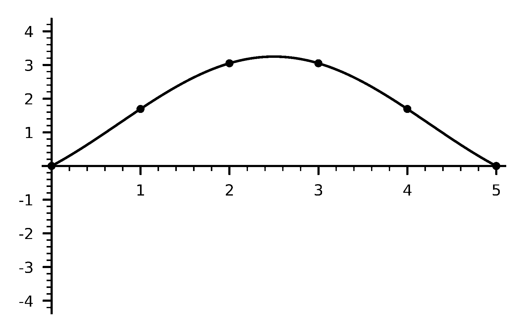 Figure 5
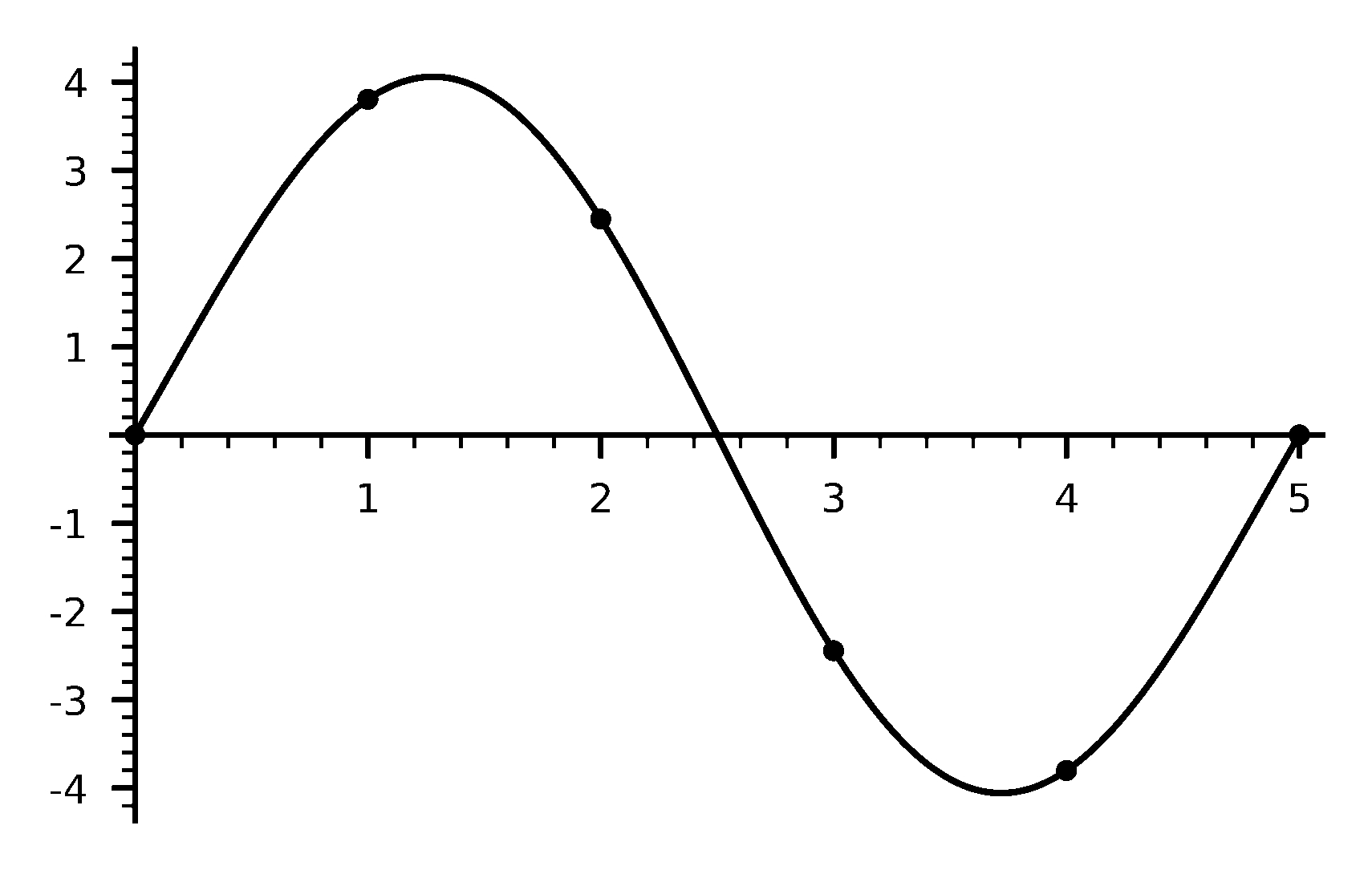 Figure 5
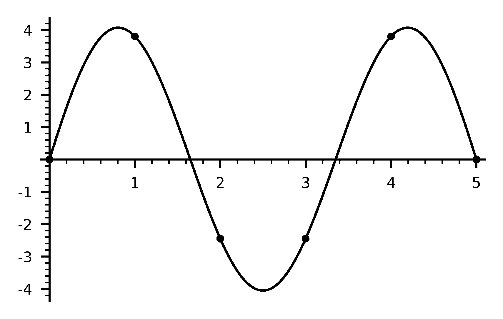 Figure 6
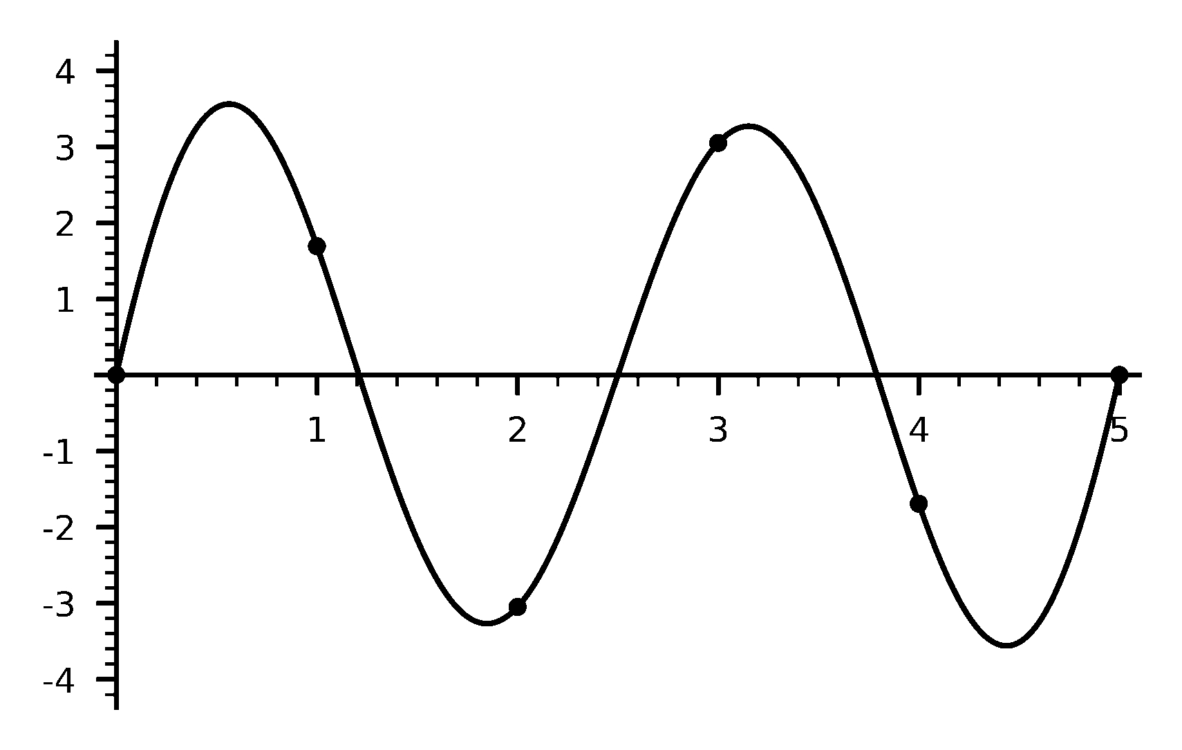 Figure 6