Fractional Piola identity and polyconvexity in fractional spaces
Jos\'e C. Bellido, Javier Cueto, Carlos Mora-Corral

TL;DR
This paper establishes the existence of minimizers for nonlocal variational problems involving fractional gradients by proving a fractional Piola identity, extending classical elasticity concepts to fractional spaces.
Contribution
It introduces the fractional Piola identity and demonstrates the existence of minimizers in fractional spaces under polyconvexity, advancing nonlocal elasticity theory.
Findings
Existence of minimizers in fractional spaces.
Fractional Piola identity ensures weak convergence of the fractional gradient determinant.
Compatibility with discontinuous solutions in nonlocal elasticity.
Abstract
In this paper we address nonlocal vector variational principles obtained by substitution of the classical gradient by the Riesz fractional gradient. We show the existence of minimizers in Bessel fractional spaces under the main assumption of polyconvexity of the energy density, and, as a consequence, the existence of solutions to the associated Euler--Lagrange system of nonlinear fractional PDE. The main ingredient is the fractional Piola identity, which establishes that the fractional divergence of the cofactor matrix of the fractional gradient vanishes. This identity implies the weak convergence of the determinant of the fractional gradient, and, in turn, the existence of minimizers of the nonlocal energy. Contrary to local problems in nonlinear elasticity, this existence result is compatible with solutions presenting discontinuities at points and along hypersurfaces.
Click any figure to enlarge with its caption.
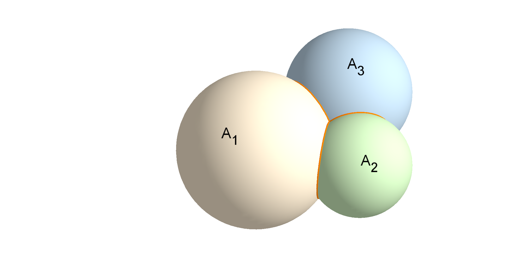 Figure 1
Peer Reviews
No public reviews on file for this paper yet. If you reviewed it on a platform where reviews are public (OpenReview, ICLR, NeurIPS, ICML), you can paste yours below so the community can read it here.
Videos
No videos yet. Explain this paper in a talk, walkthrough, or lecture? Add one.
Fractional Piola identity and polyconvexity in fractional spaces
José C. Bellido
Javier Cueto
Carlos Mora-Corral
Department of Mathematics, Universidad Autónoma de Madrid, Cantoblanco, 28.049-Madrid
E.T.S.I. Industriales, Department of Mathematics, Universidad de Castilla-La Mancha, 13.071-Ciudad Real, Spain
Abstract
In this paper we address nonlocal vector variational principles obtained by substitution of the classical gradient by the Riesz fractional gradient. We show the existence of minimizers in Bessel fractional spaces under the main assumption of polyconvexity of the energy density, and, as a consequence, the existence of solutions to the associated Euler–Lagrange system of nonlinear fractional PDE. The main ingredient is the fractional Piola identity, which establishes that the fractional divergence of the cofactor matrix of the fractional gradient vanishes. This identity implies the weak convergence of the determinant of the fractional gradient, and, in turn, the existence of minimizers of the nonlocal energy. Contrary to local problems in nonlinear elasticity, this existence result is compatible with solutions presenting discontinuities at points and along hypersurfaces.
keywords:
Nonlocal variational problems , Riesz fractional gradient , Fractional Piola identity , Polyconvexity
MSC:
[2010] 35Q74 , 35R11 , 49J45
1 Introduction
In the last years there has been a renewed interest in variational problems involving the so-called Riesz -fractional gradient, which for a function is defined as
[TABLE]
where stands for the principal value centered at , and is a suitable constant. In the recent references [32, 33], variational principles for functionals depending on this fractional gradient are addressed, as well as the fractional PDE derived from those as equilibrium equations. The authors consider typical calculus of variations problems, with standard growth conditions in which the classical (local) gradient is substituted by . This naturally leads to the consideration of the space
[TABLE]
It is also of interest the affine subspace of functions verifying a complement value condition; to be precise, given and a bounded domain , we consider
[TABLE]
where stands for the complement of in . References [32, 33] deal with integral functionals of the form
[TABLE]
with -growth conditions, and prove the existence of minimizers in under the fundamental hypothesis of convexity of in the last variable, as well as natural coercivity conditions. Taking advantage of the fractional framework and the properties of Riesz potentials and Fourier transform, they also show some remarkable results on the functional spaces , including a fractional Sobolev-type inequality, the compact embedding into and the equivalence with Bessel spaces (see [1, 38, 28]). The book [26, Ch. 15] also pays attention to the -fractional gradient, providing a proof not based on Fourier transform of a fractional fundamental theorem of calculus, also proved in [32], which is used for showing a Sobolev type inequality from to . Another reference also dealing with the fractional gradient in the case is [29].
Even more recent references are [8, 35]. In [35], the -fractional gradient together with the -fractional divergence are studied in a systematic manner. Several important properties are given, such as the uniqueness up to a multiplicative constant of the fractional gradient under natural requirements (invariance under translations and rotations, homogeneity under dilations and some continuity properties in an appropriate functional space), and some fractional calculus rules. The results in [35] established, both from a mathematical and physical perspective, what was pointed out earlier in [32, 33, 26], namely, that the -fractional gradient is the natural definition for a fractional differential object. We agree with the previous references on the claim that the -fractional gradient deserves more attention in the literature, and likely there will be both more theoretical studies and applications in different contexts. In [8], it is addressed the space of functions whose total fractional variation is finite, naturally leading to the definition of the space and to a -fractional Caccioppoli perimeter concept. Several interesting results are shown, including a continuous embedding of fractional Sobolev spaces into , a Sobolev-type inequality, a coarea formula, a -fractional isoperimetric inequality and a natural -fractional analogue of De Giorgi’s notion of reduced boundary.
The definition of the fractional gradient (1) has an important drawback when thinking about certain applications, for instance, in nonlocal solid mechanics, since it requires an integration in the whole space for the computation of the gradient. This is somehow meaningless in those contexts and, in addition, makes it difficult the extension to more realistic boundary conditions. In [24], a definition of a nonlocal gradient in bounded or unbounded domains, for which (1) is a particular case, is introduced. Moreover, the localization of this nonlocal gradient when the nonlocality parameter (horizon) goes to zero is analyzed, showing the convergence to the local gradient in different topologies. For a domain , the nonlocal gradient is defined as
[TABLE]
where the function , typically radial, is an integral kernel reflecting the forces of interaction exerted by particles separated by a positive distance smaller than . Typically vanishes outside the ball of radius centered at the origin. The oldest references we are aware of regarding nonlocal gradients of this kind used for models in continuum mechanics are [13, 12], where a nonlocal model of elasticity was proposed. More recently, a nonlocal alternative theory in solid mechanics, named peridynamics, has been proposed in [37, 36]. The development of peridynamics in the last years has been impressive; however, most of the work until now concerns linear elastic models. In [22, 23], a linear elasticity model in the context of peridynamics is rigorously studied, proving the existence and uniqueness of solutions and their convergence to the local Lamé system of linear elasticity as the horizon goes to zero. In these references a projected version of nonlocal gradient (3) is used in the context of the so-called state based peridynamic model. Another interesting approach going from a nonlocal peridynamic framework with finite horizon to a nonlocal fractional situation with infinite horizon in the linear case, appears in the recent references [19, 30, 31]. It is also worth mentioning [14], where both the ill- and well-posedness of the classical Eringen model of nonlocal elasticity are addressed.
In this investigation we deepen in the existence issue for vector variational problems involving the -fractional gradient, as well as the PDE derived from those as equilibrium conditions. Thus, we consider the more difficult vectorial case under conditions weaker than convexity. To be precise, we establish the existence of minimizers in under the polyconvexity assumption of the integrand. Polyconvexity is a central notion in calculus of variations, with essential implications on the existence and stability of solutions in solid mechanics, and particularly in elasticity [2, 9]. In order to obtain our results, we follow the usual steps as for classical polyconvex variational problems, namely, we show that the determinant (or any minor) of the fractional gradient matrix is continuous with respect to weak convergence in . Similarly to the classical case, we need a fractional version of the Piola identity, highlighting this as the key ingredient and the most remarkable contribution of this work. In this new situation we follow [24] to define a fractional divergence and establish an integration by parts formula (see also [26, 35]). We adapt the techniques developed there for some spaces of nonlocal type to our spaces. More concretely, as in (1), the Riesz -fractional gradient of a vector field is
[TABLE]
where denotes the tensor product, and the Riesz -fractional divergence of a vector field is defined as
[TABLE]
As mentioned above, we prove the fractional Piola identity (where means the -divergence by rows), then we show the weak continuity of , the weak lower semicontinuity of polyconvex functionals in , and finally we settle the existence of minimizers for (2). We believe that the fractional Piola identity is a result of interest in itself. On the one hand, it may serve to show analogous versions in the fractional or nonlocal situations of classical results in whose proof the Piola identity is invoked, as for instance, the change of variables formula for surface integrals. On the other hand, it may also be useful in other fractional or nonlocal models in different contexts, such as fluid mechanics [11]. Furthermore, an extension to a nonlocal Piola identity for nonlocal gradients defined on bounded domains (see (3)) is easy from the proof we provide here in the fractional framework.
In the last decade there has been a great deal of work on fractional PDE of elliptic type involving the fractional Laplacian in some way. Our results here enlarge this theory by giving an existence result of minimizers of nonlinear fractional vector variational problems based on polyconvexity, which implies, in turn, an existence result of solutions to nonlinear fractional PDE systems. The amount of references on nonlocal equations and fractional Laplacian is overwhelming, so for situations related to this work we just cite the survey [27], the paper [33] and the references therein. On the other hand, we would like to point out the relationship of our study with nonlocal elasticity and peridynamics. As mentioned above, the variational principle considered in this paper is not an appropriate model in solid mechanics, but a version in bounded domains of the functional (2) involving the nonlocal gradient (3), satisfying additional requirements in order to be physically consistent, fits into the peridynamics state-based model for large deformations [36]. Whereas in , the structural functional analysis facts necessary to prove an existence theory for functionals like (2) are known (continuous and compact embeddings into ), those are still unknown for an analogous version of this space in bounded domains. In this sense, and since the proof provided for the fractional Piola identity may be adapted in a more or less straightforward way to bounded domains, we think this study may be seen as a first step towards a rigorous mathematical theory of nonlocal hyperelasticity. Furthermore, one primary interest for us is that is larger than , and functions in may exhibit singularities prohibited in , as we point out in Section 2. We would like to emphasize that, contrary to classical elasticity, both singularities along points (cavitation) and hypersurfaces are compatible with the existence of solutions in (see Theorem 6.1). This seems to indicate that the norm of not only contributes to the elastic energy, but also to a kind of surface energy, since the latter is necessary in the modelling of such singularities (see, e.g., [4, 25, 10, 18]).
The outline of the paper is the following. Section 2 introduces the functional space of fractional type and its main properties. We also include examples of functions exhibiting singularities belonging to these spaces but not to Sobolev spaces. Section 3 contains some calculus facts in , such as the formulas for the fractional derivative of a product and the fractional integration by parts. In Section 4 we prove the fractional Piola identity. Section 5 shows the weak continuity of minors in . Finally, in Section 6 we prove the existence of minimizers of (2) for polyconvex integrands, and obtain the associated Euler–Lagrange system of fractional PDE.
2 Functional analysis framework
This section introduces general properties of the functional space . We start by setting the definition of principal value. Given a function and such that for every , we define the principal value centered at of , denoted by
[TABLE]
as
[TABLE]
whenever this limit exists. We have denoted by the open ball centered at of radius , and by its complement. As most integrals in this work are over , we will use the symbol as a substitute for .
The -fractional gradient is defined as follows.
Definition 2.1**.**
Let be a measurable function. Let and be such that
[TABLE]
for each . Set
[TABLE]
where is the Euler gamma function. We define , the -fractional gradient of at , as
[TABLE]
whenever the principal value exists.
We note that, due to symmetry,
[TABLE]
and consequently, the equality
[TABLE]
holds. Notice also that the constant is negative.
Definition 2.1 naturally extends to vector fields. Given measurable such that (4) holds for each , its -fractional gradient is
[TABLE]
whenever it exists. Here, stands for the tensor product of vectors. Given and , we define the space as
[TABLE]
and we denote . We will study complement value problems (as in, for example, [16]), so we are interested in the case in which functions are prescribed in the complement of a given set. Thus, given an open set and , the space is defined as
[TABLE]
The space , together with the -fractional gradient as a mathematical object, was introduced and studied in [32, 33] (see also [26, Sect. 15.2]). The first remarkable fact is the identification of with the classical Bessel potential spaces (see [1, 38, 28]) established in [32, Th. 1.7]. Thanks to this equivalence, and rewriting well-known properties for Bessel spaces in terms of spaces, we obtain several basic properties that we summarize in the following proposition (see [1, Ch. 7, p. 221]). We denote by continuous inclusion.
Proposition 2.1**.**
Set and . Then:
- a)
* is dense in .* 2. b)
* is reflexive.* 3. c)
If and , then . 4. d)
If , then . 5. e)
If , then with equivalence of norms. 6. f)
If then .
We have denoted by the classical fractional Sobolev space. Although they will not be used in this paper, they were mentioned in Proposition 2.1 to help locate the spaces in a more familiar scale of regularity. We have also denoted by the space of Hölder continuous functions of exponent .
An essential tool for obtaining existence of minimizers for variational functionals is a Poincaré-type inequality. Collecting together several theorems present in the literature, we state the following result, which is not optimal but suitable for our purposes. Henceforth, given and with we define .
Theorem 2.2**.**
Set and . Let be a bounded open set. Then there exists such that
[TABLE]
for all , and any satisfying
[TABLE]
The case is an immediate consequence of [32, Th. 1.8], where the continuous embedding of in is shown. Case is a consequence of [32, Th. 1.10], where it is proved in this context the version of Trudinger’s inequality, which implies the embedding of in for all . Finally, the case is a consequence of Proposition 2.1 d).
The following result decides which of the embeddings of Theorem 2.2 are compact. We will indicate by weak convergence.
Theorem 2.3**.**
Set and . Let be open and bounded and . Then for any sequence such that
[TABLE]
for some , one has and
[TABLE]
for every satisfying
[TABLE]
Case is actually [33, Th. 2.2]. Case follows from the former having in mind Proposition 2.1, part c) or else part f). Finally, the case is a consequence of Proposition 2.1 d) and the compact embedding of into .
It is worth mentioning that case is intentionally avoided. First, because the original statements of Proposition 2.1 and Theorems 2.2 and 2.3 exclude this case, and, second, because we are concerned with a general existence theory that requires reflexive spaces.
2.1 Examples of functions in
One of the motivations of this study is to propose an existence theory formulated in spaces wider than classical Sobolev spaces. As a consequence of Proposition 2.1 f), classical Sobolev spaces are continuously embedded in spaces. Further, we are interested in functions that belong to but not to . Necessarily, those functions must exhibit some type of singularity. We focus on two important singularities in solid mechanics: discontinuities along hypersurfaces and at a single point. The later corresponds with the paradigmatic case of cavitation. For simplicity, we study as a model for singularities along hypersurfaces a function whose first component is the characteristic function of the unit cube , while the other components are functions. As a model for singularity at a point, we study a radial function of compact support exhibiting one cavity at the origin. In both examples the functions have compact support: this simplifies the analysis since it avoids the issue of the integrability at infinity, and, hence, allows us to focus solely on the singularity.
We start with the case of singularity along a hypersurface. There is an extensive literature on when the characteristic function of a set (especially, of an open bounded Lipschitz set) belongs to a functional space of fractional regularity (see, e.g., [39, 28, 34, 21, 15]). We exploit those results to give a quick proof of the following lemma.
Lemma 2.4**.**
Set and . Let and . Define . Then
[TABLE]
Proof.
As (we will show this in Lemma 3.1), we have that if and only if .
The fractional Sobolev space coincides with the Triebel–Lizorkin space and with the Besov space (see, e.g., [39, Sect. 2.3.5] or [28, Prop. 2.1.2]). This result together with [28, Lemma 4.6.3.2] shows that if and only if . Proposition 2.1 f) concludes the proof. ∎
For the case of cavitation, the result is the following.
Lemma 2.5**.**
Set and . Let be such that , and . Then
[TABLE]
Proof.
It is well known that whenever (see, e.g., [3, Lemma 4.1]), and therefore for any and . Applying now Proposition 2.1 c), we have that for any and . Now we observe that the set of such that there exist and for which and is precisely the set of such that and . Therefore, if .
On the other hand, when , by Proposition 2.1 d), functions are continuous. Since is discontinuous, if . ∎
3 Calculus in
In this section we present some calculus rules of nonlocal functionals related to , notably, an integration by parts formula.
We start with a sufficient condition for the -fractional gradient to be defined everywhere.
Lemma 3.1**.**
Let and . Then
[TABLE]
If, in addition, has compact support then , for every .
Proof.
Let and be, respectively, the Lipschitz and -Hölder constants of . Then, for every ,
[TABLE]
This means that .
Next we are going to see that when has compact support. Denote by the support of . Then
[TABLE]
where
[TABLE]
Now, we observe that, applying Fubini’s Theorem and (7),
[TABLE]
We notice that for every . Therefore, applying again (7) we get
[TABLE]
As a consequence of (8) and (9), . Finally, through a standard interpolation argument, we get that for all . ∎
Lemma 3.1 implies, in particular, that is defined everywhere for and . It also shows that for every and .
The following result defines a nonlocal operator related to the -fractional gradient.
Lemma 3.2**.**
Let and . Let and . Then, the operator defined as
[TABLE]
is linear and bounded.
If, in addition, has compact support then is bounded from to for all .
Proof.
Let . We denote by a positive constant that does not depend on and whose value may vary along the proof. For a.e. we have
[TABLE]
so
[TABLE]
with
[TABLE]
Let be a Lipschitz and an -Hölder constant of . Then, using that is Lipschitz and applying Hölder’s inequality, we get
[TABLE]
Integrating,
[TABLE]
As for the term , using that is -Hölder and applying Hölder’s inequality,
[TABLE]
Integrating,
[TABLE]
Putting together (10), (11) and (12) we obtain
[TABLE]
and the first part of the proof is finished.
Next we are going to see that the linear operator is bounded in the case has compact support. Denote by the support of . Then
[TABLE]
where
[TABLE]
Now, we observe that, applying Fubini’s Theorem, Hölder’s inequality and Lemma 3.1,
[TABLE]
We notice that for every . Therefore, applying Hölder’s inequality and Lemma 3.1 we get
[TABLE]
Using again Hölder’s inequality, Lemma 3.1 and Fubini’s Theorem, we obtain
[TABLE]
where denotes the measure of . Inequalities (13), (14) and (15) lead us to
[TABLE]
Finally, through a standard interpolation argument, we get that is bounded from to for all . ∎
As a consequence of Lemma 3.2 and a general result, the operator is continuous from the weak topology of to the weak topology of and, in the case of a of compact support, from the weak topology of to the weak topology of for all .
The next lemma finds out the spaces where the sequence is convergent, provided that is convergent in .
Lemma 3.3**.**
Let and . Let and let be a sequence converging to in . Assume that there is a compact such that . Then in for every .
Proof.
By linearity, we can assume that . Call . Then
[TABLE]
where denotes the Lebesgue measure of , and is the conjugate exponent of .
On the other hand, for every , we use Fubini’s Theorem and Hölder’s inequality to get
[TABLE]
Now, for every we have , so
[TABLE]
Now, we will use to denote a constant (depending on , and ) which can vary through the proof. So, continuing from (17) and applying Hölder’s inequality again, we obtain
[TABLE]
where we have used Proposition 2.1 f) in the last step. This inequality, together with (16), leads to
[TABLE]
by assumption. Finally, through a standard interpolation argument, we obtain the convergence in for every . ∎
Now we introduce a product formula for the -fractional gradient. We denote by the identity matrix of dimension .
Lemma 3.4**.**
Let and . Let and . Then and for a.e. ,
[TABLE]
Proof.
Clearly . Now, for a.e. we have
[TABLE]
The term is in since , while the term is in by Lemma 3.2. ∎
Inspired by [24] (see also [26]) we introduce the -fractional divergence .
Definition 3.1**.**
Let be measurable. Let and be such that
[TABLE]
for each . The -fractional divergence of is defined as
[TABLE]
whenever the principal value exists.
Analogously, if is such that its rows satisfy the assumptions of Definition 3.1, we denote by the column vector-function whose components are the -fractional divergences of each row of .
Similarly to what happened with the -fractional gradient (see (5)), by symmetry, we have that
[TABLE]
An initial property of the -fractional divergence is the following, which states that it is well defined if and only if so is the -fractional derivative. Its proof is analogous to that of [24, Lemma 2.3], and, hence, it will be omitted.
Lemma 3.5**.**
Let be measurable and let be such that is defined and finite. Then
[TABLE]
exists and is finite if and only if
[TABLE]
exists and is finite. Moreover, in this case,
[TABLE]
The most important fact relating the -fractional gradient and the -fractional divergence is the integration by parts formula. The proof of this result follows the lines of [24, Th. 1.4].
Theorem 3.6**.**
Let . Let be such that
[TABLE]
for every compact . Then and for all ,
[TABLE]
Proof.
Assumption (19) implies that exists a.e. as a Lebesgue integral and , we have
[TABLE]
On the other hand, as , by Lemma 3.5,
[TABLE]
Thus, it suffices to establish the equality of the right hand sides of (20) and (21); in fact, we will establish the equality of the double integrals in the domain for each . We have
[TABLE]
If we interchange now the roles of and in the second integral, using the symmetry of , we have
[TABLE]
and therefore
[TABLE]
whence the equality of the right hand sides of (20) and (21) follows. ∎
As in Lemma 3.4, the following result computes the -fractional divergence of a product.
Lemma 3.7**.**
Let and . Let and . Then and for a.e. ,
[TABLE]
4 Fractional Piola Identity
In this section we introduce a fractional version of the Piola Identity. This is the main step in order to prove the existence of solutions for our fractional energy, since it will allow us to prove the weak continuity in of the determinant of the -fractional gradient. Recall that the classical Piola identity asserts that, for smooth enough functions one has . Of course, denotes the cofactor matrix, which satisfies for every .
Contrary to the classical case, the proof of the fractional Piola identity is not trivial even for smooth functions. Indeed, the classical proof cannot be reproduced in this case as it relies on Leibniz’s rule and symmetry of second derivatives. Notice that Lemma 3.7 prevents all the terms of the second derivatives from being cancelled as happens in the classical case. In the next lines we sketch a possible proof of this identity in order to find out the difficulties. We emphasize that the next argument is formal in order to illustrate the difficulties for proving the fractional Piola identity. The main assumption we make is that all integrals involved are absolutely convergent without the need of the principal value, so that we can apply Fubini’s theorem. Starting from (5), we have
[TABLE]
For simplicity in the calculations, we set , the simplest case. Then the first row of is
[TABLE]
and, using (18), the first component of is
[TABLE]
Now, for every and ,
[TABLE]
because of the odd symmetry of the integral. Notice that the integrals in (22) are not defined as Lebesgue integrals. The real proof will consist in making these calculations rigorous for arbitrary dimension . The underlying reason of why the fractional Piola identity is true is that is a sort of null Lagrangian in the sense that, for any , the integral
[TABLE]
is zero. This is a consequence of the fact that the determinant is an alternating multilinear form, as well as that is a classical null Lagrangian. However, as we will see in Lemma 4.1, the previous integral is not defined as a proper integral but as a principal value centered at points , and this will cause technical difficulties in the proof.
We start by reviewing a version of the change of variables formula for surface integrals (see, e.g., [25, Prop. 2.7]). Let be an oriented -dimensional manifold with continuous unit normal field . Let be affine and injective, with corresponding linear map . Let be smooth. Then
[TABLE]
where denotes the surface element. Now assume that is a symmetry across a hyperplane, so , and . Therefore,
[TABLE]
Thus
[TABLE]
As this is true for every , we have that
[TABLE]
which is the formula we will use in Lemma 4.1.
In this and the next sections we will employ the following notation for the submatrices.
Definition 4.1**.**
Let be with . Consider indices and .
- a)
We define as the map such that is the submatrix of formed by the rows and the columns . 2. b)
We define as the map such that is the matrix whose rows and columns coincide with those of , whereas the rest of the entries are zero. 3. c)
We define as the map such that is the subvector of formed by the entries . 4. d)
We define as the map such that is the vector whose entries coincide with those of , whereas the rest of the entries are zero. 5. e)
We define as .
The following formulas for the determinant will be useful. Given , we express it as
[TABLE]
where are its rows. Then for each , where denotes the -th row of . Now we realize that if and
[TABLE]
then
[TABLE]
The following lemma is the rigorous version of (22).
Lemma 4.1**.**
Let be with . Consider indices and let be the function of Definition 4.1. Then there exists a continuous function such that for any and we have
[TABLE]
Proof.
We can assume that the points do not lie on an affine manifold of dimension , since otherwise for all .
Define as
[TABLE]
and as , for each . Define componentwise as . Then
[TABLE]
Call and denote by the submatrix of formed by the columns . Then, for all ,
[TABLE]
As DH\in L^{p}\bigl{(}\bigl{(}\bigcup_{j=1}^{k}B(a_{j},\epsilon_{j})\bigr{)}^{c},\mathbb{R}^{n\times n}\bigr{)} for all , we have \det D_{\vec{\jmath}}H\in L^{1}\bigl{(}\bigl{(}\bigcup_{j=1}^{k}B(a_{j},\epsilon_{j})\bigr{)}^{c}\bigr{)}. Therefore,
[TABLE]
As is smooth outside , we have that
[TABLE]
where indicates the first row of , and is the function of Definition 4.1. Let be big enough so that . Then, by the divergence theorem,
[TABLE]
where in for , and in . Having in mind the expressions (25) and (26), we find that, for some constant ,
[TABLE]
which goes to zero as . Therefore,
[TABLE]
For each we set
[TABLE]
As a consequence of the inclusion , we have that
[TABLE]
Moreover, the -dimensional area of is zero for . Figure 1 illustrates this situation when .
Next, using (24) and (26), we have that for and ,
[TABLE]
As a result, recalling (28) and the inclusion , we have that
[TABLE]
Having in mind the expression (25), the multilinearity of the determinant and considering (24) and (26), we have that, for ,
[TABLE]
where is the function of Definition 4.1.
Let be the only hyperplane in passing through the points , and consider one of the two unit normals to . Let be the symmetry with respect to , so that for every ,
[TABLE]
Let , and let be the affine hyperplane in with normal passing through . Consider as the symmetry across . Then, for all ,
[TABLE]
Let be such that the points do not lie in an affine manifold of dimension . Define . Then , and cover up to a set of zero -measure; see Figure 2.
Using the change of variables formula (23), we obtain
[TABLE]
Now, thanks to (24), for ,
[TABLE]
Let be the linear map corresponding to the affine map , and, analogously, the linear map corresponding to . We notice that . Having in mind (31) and (32), we find that
[TABLE]
and
[TABLE]
from which we deduce that . Thus,
[TABLE]
Putting together (33), (34) and (35), we obtain that
[TABLE]
Consequently, when we define as
[TABLE]
we have that
[TABLE]
For every , we join with by a curve inside , and note that the length of can be taken to be bounded by . Accordingly, let be of class such that , and is constant with . Then
[TABLE]
We calculate
[TABLE]
Now, as for every and ,
[TABLE]
so with (37) we obtain that
[TABLE]
On the other hand, for all ,
[TABLE]
Putting together (27), (29), (30), (36), (38) and (39), as well as the fact that the -dimensional area of is bounded by a constant times , we obtain that, for a constant depending on and ,
[TABLE]
The existence of the function of the statement follows. ∎
We are in a position to prove the fractional Piola Identity. Henceforth, denotes the support of a function.
Theorem 4.2**.**
Let be with . Consider indices and and the functions
[TABLE]
of Definition 4.1. Let and . Then
[TABLE]
Proof.
Let
[TABLE]
be the maps of Definition 4.1. Naturally, if and only if
[TABLE]
We shall show . The rest of the rows would proceed analogously.
Using (18), we have that, for a.e. ,
[TABLE]
Now, by (24) and (5), we have that for a.e. ,
[TABLE]
where for each and , we have defined by
[TABLE]
and we have used the continuity of the determinant. Let be such that for all , and fix . By odd symmetry, we have that
[TABLE]
so, using the fact that is Lipschitz, we have, for some constant , that
[TABLE]
This shows that
[TABLE]
for some only depending on and . As
[TABLE]
for any , we can apply dominated convergence to conclude that
[TABLE]
Recalling (40) and (41), with this we obtain that
[TABLE]
Now for every we define and have that, thanks to the multilinearity of the determinant,
[TABLE]
Set
[TABLE]
Then,
[TABLE]
Thanks to Lemma 4.1,
[TABLE]
where is the function that appears therein. Integrating in (44), we find that
[TABLE]
for some continuous function . Consequently,
[TABLE]
and, in view of (42) and (43), we obtain that . ∎
5 Weak continuity of the determinant
In this section we prove that any minor (determinant of a submatrix) of is a weakly continuous mapping in . We start by expressing a nonlocal integration by parts formula for the minors of that involves the operator of Lemma 3.2. Recall that for any and we denote by the -th row of .
Lemma 5.1**.**
Let be with . Consider indices and and the functions
[TABLE]
of Definition 4.1. Let , and . Let be such that . Then, , and for every we have that and
[TABLE]
Proof.
The fact is a consequence of formula (24) and Hölder’s inequality, since . Moreover, , since and for all thanks to Lemma 3.2.
Assume first and let . Fix and . By Lemma 3.7 and Theorem 4.2,
[TABLE]
When we apply Theorem 3.6 to the constant function , we obtain from integration of the previous formula that
[TABLE]
By Fubini’s theorem and the definitions of and fractional gradient,
[TABLE]
We thus have the equality
[TABLE]
Now we assume that with , and, again . Taking into account Proposition 2.1, let be a sequence in converging to in . Then in and, hence, in , so in . Therefore, (46) holds as well, since for all (see Lemma 3.1). Now let be of compact support, and let be a sequence in converging to in such that is bounded. Then, by Lemma 3.3, in for all . As , we have that (46) holds as well. To sum up, formula (46) is valid for any with and any of compact support.
We apply (46) to , which is in thanks to Lemma 3.4, and has compact support since so does . By the formula for given by Lemma 3.4, we obtain that
[TABLE]
Using formula (24), the fact and elementary properties of the functions of Definition 4.1, we find that for any ,
[TABLE]
Using this and Fubini’s theorem, from (47) we arrive at
[TABLE]
We sum this equality for and obtain that
[TABLE]
which is the required formula. ∎
Now we establish the closedness and continuity properties of the minors of in the weak topology of . In the notation of Definition 4.1 a), a minor of order is a function such that there exist and for which for all . Recall the notation of Theorem 2.2, and the affine space of (6).
Theorem 5.2**.**
Let and . Let and . Let be a sequence in such that in . Then
- a)
If with and is a minor of order then in as . 2. b)
If in for some and then . 3. c)
Assume in for some and some . If assume, in addition, that in for some . Then .
Proof.
We will prove a) by induction on . For the result is trivial. Assume it holds for some and let us prove it for . Let be a minor of order . In the notation of Definition 4.1 a), for all , where for some and . Let . By induction assumption, in as , so in . By Lemma 3.2, in for every . By Theorem 2.3, in , so
[TABLE]
since . We apply Lemma 5.1 and, in particular, formula (45) to conclude that
[TABLE]
This shows that in the sense of distributions. As is bounded in and , we have that in .
The proof of b) follows the lines of a). Let be a minor of order . In the notation of Definition 4.1 a), for all , where for some and . Let . By part a), in , so in . By Lemma 3.2, in for every . By Theorem 2.3, in , so convergence (48) is also valid since . Thanks to (45), we conclude that convergence (49) holds. This shows that in the sense of distributions. As this is true for every minor of order , we obtain that in the sense of distributions. Thanks to the assumption, .
We finally show part c). Let . Assume first . By the assumption and Lemma 3.2, in for every . By Theorem 2.3, in for every , so
[TABLE]
since .
Assume now . Then is bounded in so, thanks to part b), in . By Lemma 3.2, in for every . By Theorem 2.3, in for every , so convergence (50) holds since .
In either case, we have convergence (50), so by (45) we obtain
[TABLE]
This shows that in the sense of distributions, so . ∎
Remark 5.1**.**
A natural question is whether the weak continuity of the determinant of the fractional gradient may be concluded as a consequence of the weak continuity of the determinant of the classical gradient. Indeed, one can use the properties of the Riesz potential to give a simpler proof in the case . To be precise, in [8, Prop. 2.2] (see also [32, Th. 1.2]) it is shown that
[TABLE]
for any , where . Now, writing the determinant as a divergence [2, Sect. 6] and using (51), we have that
[TABLE]
for any and any test function . By density of in , equality (52) holds for any . Now, taking into account the Hardy–Littlewood–Sobolev embedding [38, Th. 1, b)], and Theorem 2.2 it is easy to obtain the weak continuity of in for . We do not know whether it is possible to extend the previous argument for without making use of the fractional Piola identity.
6 Existence of minimizers and equilibrium conditions
In this section we prove the existence of minimizers in of functionals of the form
[TABLE]
under natural coercivity and polyconvexity assumptions. We also derive the associated Euler–Lagrange equation, which is a fractional partial differential system of equations.
We recall the concept of polyconvexity (see, e.g, [2, 9]). Let be the number of submatrices of an matrix. We fix a function such that is the collection of all minors of an in a given order. A function is polyconvex if there exists a convex such that for all .
The existence theorem of this paper is as follows. Its proof relies on a standard argument in the calculus of variations, once we have the continuity (with respect to the weak convergence) of the minors given by Theorem 5.2.
Theorem 6.1**.**
Let satisfy and . Let satisfy the following conditions:
- a)
* is -measurable, where denotes the Lebesgue sigma-algebra in , whereas and denote the Borel sigma-algebras in and , respectively.* 2. b)
* is lower semicontinuous for a.e. .* 3. c)
For a.e. and every , the function is polyconvex. 4. d)
There exist a constant , an and a Borel function such that
[TABLE]
and
[TABLE]
for a.e. , all and all .
Let be a bounded open subset of . Let . Define as in (53), and assume that is not identically infinity in . Then there exists a minimizer of in .
Proof.
Assumption d) shows that the functional is bounded below by . As is not identically infinity in , there exists a minimizing sequence of in . Assumption d) implies that is bounded in . Thanks to Theorem 2.2, is bounded in . As in for all , we also have that is bounded in , and, consequently, also in . As is reflexive, we can extract a weakly convergent subsequence. Using Theorem 2.3, we obtain that there exists such that for a subsequence (not relabelled),
[TABLE]
Now, by Theorem 5.2, for any minor of order , we have that
[TABLE]
If then, by assumption d), is bounded in , whereas if we call and have that is bounded in . In either case we have that , so for a subsequence converges weakly in and, by Theorem 5.2,
[TABLE]
If then, by assumption d) and de la Vallée Poussin’s criterion, is equiintegrable, whereas if we have that is bounded in and . In either case we have that, for a subsequence converges weakly in with
[TABLE]
and, hence, by Theorem 5.2,
[TABLE]
Convergences (54)–(57) imply, thanks to a standard lower semicontinuity result for polyconvex functionals (see, e.g., [6, Th. 5.4] or [17, Th. 7.5]), that for any ,
[TABLE]
Therefore,
[TABLE]
By monotone convergence,
[TABLE]
so
[TABLE]
Therefore, is a minimizer of in and the proof is concluded. ∎
Comparing Lemmas 2.4 and 2.5 with Theorem 6.1, we see that functions exhibiting singularities as those shown in those lemmas are compatible with the existence result of Theorem 6.1, in opposition to the case of classical elasticity (see, e.g., [2, 3, 4, 5, 18, 7]). Indeed, for a of compact support and , by Hölder’s inequality and Lemma 3.3, for every and for every . Take now an such that , so that this regime is compatible with cavitation (see Lemma 2.5). Considering the function of Theorem 6.1 as , we see that this map is compatible with the assumptions of Theorem 6.1 if and only if , so . To sum up, in the regime
[TABLE]
a typical cavitation map is compatible with the hypothesis of Theorem 6.1. Similarly, if and , i.e., in the regime
[TABLE]
the hypothesis of Theorem 6.1 are compatible with discontinuities along hypersurfaces.
To finish the article, we explore the equilibrium conditions that minimizers of functional (53) satisfy. This Euler–Lagrange, or equilibrium, conditions constitute a nonlinear system of fractional PDE, and therefore we are providing an existence result for such kind of systems based on polyconvexity. To be precise, given , the boundary value problem reads as
[TABLE]
Inspired by Theorem 3.6, we define a weak solution of (58) as a satisfying
[TABLE]
for all with in .
The derivation of (59) for a minimizer is standard. For this, we make the assumptions a–b) below, which are slightly adapted from [9, Conditions 3.22 and 3.33], although other sets of assumptions are also possible (see, e.g., [2, Sect. 7] or [9, Sect. 3.4.2]).
Theorem 6.2**.**
Let be a function satisfying
- a)
* is measurable for every and is of class for a.e. .* 2. b)
There exist an , an with
[TABLE]
and a such that
[TABLE]
for a.e. and all .
Let . Define as in (53), and let be a minimizer of in . Then is a weak solution of (58).
Proof.
Let us fix with in . As for any , it suffices to show that the derivative of exists at and equals the left hand side of (59). Thanks to the dominated convergence theorem, it suffices to show (see, e.g., [20, Ch. 13, §2, Lemma 2.2]) that there exists such that for every with we have
[TABLE]
and
[TABLE]
Let us check condition (60). Thanks to b) ,
[TABLE]
for some constant . Clearly, the integral of is finite since , and so is the integral of due to Lemma 3.1. In addition, the integral of is finite because . Now, by Theorem 2.2 and the interpolation (or Hölder) inequality, for all if , and for all if . Therefore, . Condition (60) is thus satisfied.
We now show condition (61). We have, for and a.e. ,
[TABLE]
where we have used Lemma 3.1 to show that . Now, by b),
[TABLE]
for some constant . As before, the right hand side of (62) is in , so condition (61) is proved. ∎
Acknowledgements
This work has been supported by the Spanish Ministerio de Ciencia, Innovación y Universidades through projects MTM2017-83740-P (J.C.B. and J.C.), and MTM2017-85934-C3-2-P (C.M.-C.).
References
- Adams [1975]
Adams, R. A., 1975. Sobolev spaces. Vol. 65 of Pure and Applied Mathematics. Academic Press, New York-London.
- Ball [1977]
Ball, J. M., 1977. Convexity conditions and existence theorems in nonlinear elasticity. Arch. Rational Mech. Anal. 63 (4), 337–403.
URL https://doi.org/10.1007/BF00279992
- Ball [1982]
Ball, J. M., 1982. Discontinuous equilibrium solutions and cavitation in nonlinear elasticity. Philos. Trans. R. Soc. Lond. Ser. A 306, 557–611.
- Ball [2001]
Ball, J. M., 2001. Singularities and computation of minimizers for variational problems. In: Foundations of computational mathematics (Oxford, 1999). Vol. 284 of London Math. Soc. Lecture Note Ser. Cambridge Univ. Press, Cambridge, pp. 1–20.
- Ball [2002]
Ball, J. M., 2002. Some open problems in elasticity. In: Geometry, mechanics, and dynamics. Springer, New York, pp. 3–59.
URL https://doi.org/10.1007/0-387-21791-6_1
- Ball et al. [1981]
Ball, J. M., Currie, J. C., Olver, P. J., 1981. Null Lagrangians, weak continuity, and variational problems of arbitrary order. J. Funct. Anal. 41 (2), 135–174.
URL https://doi.org/10.1016/0022-1236(81)90085-9
- Barchiesi et al. [2017]
Barchiesi, M., Henao, D., Mora-Corral, C., 2017. Local invertibility in Sobolev spaces with applications to nematic elastomers and magnetoelasticity. Arch. Rational Mech. Anal. 224 (2), 743–816.
URL http://dx.doi.org/10.1007/s00205-017-1088-1
- Comi and Stefani [2019]
Comi, G. E., Stefani, G., 2019. A distributional approach to fractional Sobolev spaces and fractional variation: Existence of blow-up. J. Funct. Anal.
URL http://www.sciencedirect.com/science/article/pii/S0022123619301016
- Dacorogna [2008]
Dacorogna, B., 2008. Direct methods in the calculus of variations, 2nd Edition. Vol. 78 of Applied Mathematical Sciences. Springer, New York.
- Dal Maso et al. [2005]
Dal Maso, G., Francfort, G. A., Toader, R., 2005. Quasistatic crack growth in nonlinear elasticity. Arch. Rational Mech. Anal. 176 (2), 165–225.
- Du and Tian [2019]
Du, X., Tian, X., 2019. Mathematics of Smoothed Particle Hydrodynamics, Part I: a nonlocal Stokes equation. To appear in Foundations in Computational Mathematics.
- Edelen et al. [1971]
Edelen, D. G. B., Green, A., Laws, N., 1971. Nonlocal continuum mechanics. Arch. Rational Mech. Anal. 43, 34–44.
- Edelen and Laws [1971]
Edelen, D. G. B., Laws, N., 1971. On the thermodynamics of systems with nonlocality. Arch. Rational Mech. Anal. 43, 24–35.
URL https://doi.org/10.1007/BF00251543
- Evgrafov and Bellido [2019]
Evgrafov, A., Bellido, J. C., 2019. From non-local Eringen’s model to fractional elasticity. Math. Mech. Solids 24 (6), 1935–1953.
URL https://doi.org/10.1177/1081286518810745
- Faraco and Rogers [2013]
Faraco, D., Rogers, K. M., 2013. The Sobolev norm of characteristic functions with applications to the Calderón inverse problem. Q. J. Math. 64 (1), 133–147.
URL https://doi.org/10.1093/qmath/har039
- Felsinger et al. [2015]
Felsinger, M., Kassmann, M., Voigt, P., 2015. The Dirichlet problem for nonlocal operators. Math. Z. 279 (3-4), 779–809.
URL https://doi.org/10.1007/s00209-014-1394-3
- Fonseca and Leoni [2007]
Fonseca, I., Leoni, G., 2007. Modern methods in the calculus of variations: spaces. Springer Monographs in Mathematics. Springer, New York.
- Henao and Mora-Corral [2010]
Henao, D., Mora-Corral, C., 2010. Invertibility and weak continuity of the determinant for the modelling of cavitation and fracture in nonlinear elasticity. Arch. Rational Mech. Anal 197, 619–655.
- Kassmann et al. [2019]
Kassmann, M., Mengesha, T., Scott, J., 2019. Solvability of nonlocal systems related to peridynamics. Commun. Pure Appl. Anal. 18 (3), 1303–1332.
- Lang [1983]
Lang, S., 1983. Real analysis, 2nd Edition. Addison-Wesley, Reading, MA.
- Maz’ya [2011]
Maz’ya, V., 2011. Sobolev spaces with applications to elliptic partial differential equations, 2nd Edition. Vol. 342 of Grundlehren der Mathematischen Wissenschaften. Springer, Heidelberg.
URL http://dx.doi.org/10.1007/978-3-642-15564-2
- Mengesha and Du [2015]
Mengesha, T., Du, Q., 2015. On the variational limit of a class of nonlocal functionals related to peridynamics. Nonlinearity 28 (11), 3999–4035.
URL https://doi.org/10.1088/0951-7715/28/11/3999
- Mengesha and Du [2016]
Mengesha, T., Du, Q., 2016. Characterization of function spaces of vector fields and an application in nonlinear peridynamics. Nonlinear Anal. 140, 82–111.
URL https://doi.org/10.1016/j.na.2016.02.024
- Mengesha and Spector [2015]
Mengesha, T., Spector, D., 2015. Localization of nonlocal gradients in various topologies. Calc. Var. Partial Differential Equations 52 (1-2), 253–279.
URL https://doi.org/10.1007/s00526-014-0711-3
- Müller and Spector [1995]
Müller, S., Spector, S. J., 1995. An existence theory for nonlinear elasticity that allows for cavitation. Arch. Rational Mech. Anal. 131 (1), 1–66.
URL https://doi.org/10.1007/BF00386070
- Ponce [2016]
Ponce, A. C., 2016. Elliptic PDEs, measures and capacities. Vol. 23 of EMS Tracts in Mathematics. European Mathematical Society (EMS), Zürich, from the Poisson equations to nonlinear Thomas-Fermi problems.
URL https://doi.org/10.4171/140
- Ros-Oton [2016]
Ros-Oton, X., 2016. Nonlocal elliptic equations in bounded domains: a survey. Publ. Mat. 60 (1), 3–26.
URL http://projecteuclid.org/euclid.pm/1450818481
- Runst and Sickel [1996]
Runst, T., Sickel, W., 1996. Sobolev spaces of fractional order, Nemytskij operators, and nonlinear partial differential equations. Vol. 3 of De Gruyter Series in Nonlinear Analysis and Applications. Walter de Gruyter & Co., Berlin.
URL https://doi.org/10.1515/9783110812411
- Schikorra et al. [2017]
Schikorra, A., Spector, D., Van Schaftingen, J., 2017. An -type estimate for Riesz potentials. Rev. Mat. Iberoam. 33 (1), 291–303.
URL https://doi.org/10.4171/RMI/937
- Scott and Mengesha [2019a]
Scott, J., Mengesha, T., 2019a. A fractional Korn-type inequality. Discrete Contin. Dyn. Syst. A 39 (6), 3315–3343.
URL http://aimsciences.org//article/id/fa5bdce1-5e95-404f-8caf-3ae336205c8d
- Scott and Mengesha [2019b]
Scott, J., Mengesha, T., 2019b. A potential space estimate for solutions of systems of nonlocal equations in peridynamics. SIAM J. Math. Anal. 51 (1), 86–109.
URL https://doi.org/10.1137/18M1189294
- Shieh and Spector [2015]
Shieh, T.-T., Spector, D. E., 2015. On a new class of fractional partial differential equations. Adv. Calc. Var. 8 (4), 321–336.
URL https://doi.org/10.1515/acv-2014-0009
- Shieh and Spector [2018]
Shieh, T.-T., Spector, D. E., 2018. On a new class of fractional partial differential equations II. Adv. Calc. Var. 11 (3), 289–307.
URL https://doi.org/10.1515/acv-2016-0056
- Sickel [1999]
Sickel, W., 1999. Pointwise multipliers of Lizorkin-Triebel spaces. In: The Maz’ya anniversary collection, Vol. 2 (Rostock, 1998). Vol. 110 of Oper. Theory Adv. Appl. Birkhäuser, Basel, pp. 295–321.
- Šilhavý [2019]
Šilhavý, M., Jun 2019. Fractional vector analysis based on invariance requirements (critique of coordinate approaches). Continuum Mechanics and Thermodynamics.
URL https://doi.org/10.1007/s00161-019-00797-9
- Silling and Lehoucq [2010]
Silling, S., Lehoucq, R., 2010. Peridynamic theory of solid mechanics. In: Aref, H., van der Giessen, E. (Eds.), Advances in Applied Mechanics. Vol. 44 of Advances in Applied Mechanics. Elsevier, pp. 73 – 168.
URL http://www.sciencedirect.com/science/article/pii/S0065215610440028
- Silling [2010]
Silling, S. A., 2010. Linearized theory of peridynamic states. J. Elasticity 99 (1), 85–111.
URL https://doi.org/10.1007/s10659-009-9234-0
- Stein [1970]
Stein, E. M., 1970. Singular integrals and differentiability properties of functions. Princeton Mathematical Series, No. 30. Princeton University Press, Princeton, N.J.
- Triebel [1983]
Triebel, H., 1983. Theory of function spaces. Vol. 78 of Monographs in Mathematics. Birkhäuser Verlag, Basel.
The reference list from the paper itself. Each links out to its DOI / PubMed record.
- 1Adams [1975] Adams, R. A., 1975. Sobolev spaces. Vol. 65 of Pure and Applied Mathematics. Academic Press, New York-London.
- 2Ball [1977] Ball, J. M., 1977. Convexity conditions and existence theorems in nonlinear elasticity. Arch. Rational Mech. Anal. 63 (4), 337–403. URL https://doi.org/10.1007/BF 00279992 · doi ↗
- 3Ball [1982] Ball, J. M., 1982. Discontinuous equilibrium solutions and cavitation in nonlinear elasticity. Philos. Trans. R. Soc. Lond. Ser. A 306, 557–611.
- 4Ball [2001] Ball, J. M., 2001. Singularities and computation of minimizers for variational problems. In: Foundations of computational mathematics (Oxford, 1999). Vol. 284 of London Math. Soc. Lecture Note Ser. Cambridge Univ. Press, Cambridge, pp. 1–20.
- 5Ball [2002] Ball, J. M., 2002. Some open problems in elasticity. In: Geometry, mechanics, and dynamics. Springer, New York, pp. 3–59. URL https://doi.org/10.1007/0-387-21791-6_1 · doi ↗
- 6Ball et al. [1981] Ball, J. M., Currie, J. C., Olver, P. J., 1981. Null Lagrangians, weak continuity, and variational problems of arbitrary order. J. Funct. Anal. 41 (2), 135–174. URL https://doi.org/10.1016/0022-1236(81)90085-9 · doi ↗
- 7Barchiesi et al. [2017] Barchiesi, M., Henao, D., Mora-Corral, C., 2017. Local invertibility in Sobolev spaces with applications to nematic elastomers and magnetoelasticity. Arch. Rational Mech. Anal. 224 (2), 743–816. URL http://dx.doi.org/10.1007/s 00205-017-1088-1 · doi ↗
- 8Comi and Stefani [2019] Comi, G. E., Stefani, G., 2019. A distributional approach to fractional Sobolev spaces and fractional variation: Existence of blow-up. J. Funct. Anal. URL http://www.sciencedirect.com/science/article/pii/S 0022123619301016