Lower Bounds on the Localisation Length of Balanced Random Quantum Walks
Joachim Asch, Alain Joye

TL;DR
This paper investigates the localization length of balanced random quantum walks on lattices and trees, deriving lower bounds and showing divergence on trees as the degree increases, with implications for quantum transport.
Contribution
It introduces a combinatorial expression for localization length and establishes lower bounds, including divergence on trees and bounds on cubic lattices, advancing understanding of quantum walk localization.
Findings
Localization length diverges on the tree as degree squared (d^2).
Lower bound of 1/ln(2) for the cubic lattice localization length.
Localization length is bounded below by the correlation length of self-avoiding walks.
Abstract
We consider the dynamical properties of Quantum Walks defined on the d-dimensional cubic lattice, or the homogeneous tree of coordination number 2d, with site dependent random phases, further characterised by transition probabilities between neighbouring sites equal to 1/(2d). We show that the localisation length for these Balanced Random Quantum Walks can be expressed as a combinatorial expression involving sums over weighted paths on the considered graph. This expression provides lower bounds on the localisation length by restriction to paths with weight 1, which allows us to prove the localisation length diverges on the tree as d^2. On the cubic lattice, the method yields the lower bound 1/ln(2) for all d, and allows us to bound the localisation length from below by the correlation length of self-avoiding walks computed at 1/(2d)
Click any figure to enlarge with its caption.
 Figure 1
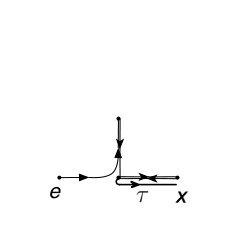 Figure 2
Peer Reviews
No public reviews on file for this paper yet. If you reviewed it on a platform where reviews are public (OpenReview, ICLR, NeurIPS, ICML), you can paste yours below so the community can read it here.
Videos
No videos yet. Explain this paper in a talk, walkthrough, or lecture? Add one.
Lower Bounds on the Localisation Length of
Balanced Random Quantum Walks
Joachim Asch , Alain Joye
Aix Marseille Univ, Université de Toulon, CNRS, CPT, Marseille, France Univ. Grenoble Alpes, CNRS, Institut Fourier, F-38000 Grenoble, France
(April 5, 2019 )
Abstract
We consider the dynamical properties of Quantum Walks defined on the -dimensional cubic lattice, or the homogeneous tree of coordination number , with site dependent random phases, further characterised by transition probabilities between neighbouring sites equal to . We show that the localisation length for these Balanced Random Quantum Walks can be expressed as a combinatorial expression involving sums over weighted paths on the considered graph. This expression provides lower bounds on the localisation length by restriction to paths with weight , which allows us to prove the localisation length diverges on the tree as . On the cubic lattice, the method yields the lower bound for all , and allows us to bound the localisation length from below by the correlation length of self-avoiding walks computed at .
1 Introduction
The last decade has seen Quantum Walks, (QWs for short), deterministic or random, play a growing role in several scientific fields, starting with the modeling of quantum dynamics in various physical situations. Let us simply mention that QWs provide a simple description of the electronic motion in the Quantum Hall geometry [CC, KOK, ABJ1], while their effectiveness in quantum optics as discrete models to study atoms trapped in time periodic optical lattices or polarized photons propagating in networks of waveguides has found experimental confirmation [ZKGS+, SVAM+]. Theoretical quantum computing is another field in which QWs prove to be useful as tools in the elaboration or assessment of quantum algorithms, see [Sa, MNRS, P]. From a mathematical perspective, QWs have been considered as non commutative analogs of classical random walks, see e.g. [Ko, SKJ, GNVW], or as subject of study in the spectral analysis of (random) unitary operators, in the line of [BHJ, CMV, J1, HJS, DFV]. See the reviews and book [V-A, J3, Si1, ABJ2] for more applications, mathematical results, and references.
The present paper addresses the mathematical (de)localisation properties of certain Random Quantum Walks (RQWs for short) defined on infinite graphs, for the discrete time random quantum dynamical system defined by the iterates of the RQW unitary operator. Anderson localisation is ubiquitous in the physics of disordered systems and has been the object of intense research since its discovery in the fifties [A-CAT], see e.g. [CL, Ki, AW]. Delocalisation of quantum particles in presence of disorder, although expected to be present in high dimensional lattices, is however difficult to exhibit; it has been proven to hold for the Anderson model on the tree, or mild variants thereof [Kl, W]. In this context, certain RQWs viewed as substitutes of the random evolution operators generated by the discrete Anderson Hamiltonians, have proven to be mathematically more tractable and to display analogous behaviours regarding the transport properties: these RQWs describe the motion of a particle with internal degree of freedom, or quantum walker, hopping on the sites an infinite underlying graph , standing for the cubic lattice or , the homogeneous tree of coordination number , in a static random environment. The internal degree of freedom, or coin state, lives in and the deterministic part of the walk is defined as follows. Given a natural basis in , the one time step unitary evolution is obtained by the action of a unitary matrix on the coin state of the particle, followed by the action of a coin state conditioned shift which moves the particle to its nearest neighbours on . Static disorder is introduced in the model via i.i.d. random phases used to decorate the coin matrix in such a way that the unitary coin state update becomes site-dependent and random. The coin matrix of the resulting random unitary operator , called the skeleton, is a parameter which, in a sense, monitors the strength of the disorder; see the next section for precise definition.
Restricting attention to RQWs constructed this way, we recall some of their properties. RQWs defined on the one dimensional lattice exhibit dynamical localisation for all non-trivial choice of skeleton , [JM, ASW], see also [B et al] for results on CMV matrices by a different approach. Moreover, RQWs that have skeleton close to certain permutation matrices are known to exhibit dynamical localisation on the cubic lattice , [J2, J3]; a result analogous to the strong disorder regime in the Anderson model framework. To complete the analogy, RQW’s defined on homogeneous trees are proven to undergo a localisation-delocalisation spectral transition in [HJ1], when the skeleton moves from neighbourhoods of certain permutation matrices to neighbourhoods of other permutation matrices, akin to the spectral transition occurring for the Anderson model on the tree as a function of the strength of the disorder [W]. See also [ABJ3] for delocalisation results of a topological nature for the Chalker Coddington model.
The goal of the present paper is to analyse the unitary operator in case the skeleton lies as far as possible from the permutation matrices, for which localisation results hold, and to investigate the possible delocalisation properties of those RQWs. Therefore we consider RQWs associated to balanced skeletons characterised by the fact that in the natural basis the moduli of its entries are all equal to . This amounts to saying that the quantum mechanical transition probabilities induced by between neighbouring sites are all equal to , irrespective of the realisation of the random phases decorating the balanced skeleton. Such RQWs are called Balanced Random Quantum Walks, BRQWs for short. That BRQWs are likely to exhibit delocalisation properties on the cubic lattice is not granted. However, numerics obtained for the Chalker-Coddington model suggest delocalisation for values of the parameters of the model that correspond, essentially, to the balanced behaviour introduced above, see [KOK]; hence, the analogy is tempting. When considered on the tree , BRQWs are thus neither related to localisation, nor to delocalisation, a priori, and correspond to values of the parameter that are not covered by the analysis of [HJ1].
Our results concern lower bounds on the localisation length of BRQWs defined on the cubic lattice or the tree , making use of two characteristic specificities of BRQWs operators: uniform transition probabilities between neighbouring sites and uniform distribution of the iid random phases. The localisation length we consider is defined, informally, as the inverse of the largest such that , for all initial states supported on a single site of with given internal degree of freedom, and is the multiplication operator by the norm of the position on . The localisation length defined similarly for compactly supported initial states is then bounded below by the one we consider. The fact that RQWs couple nearest neighbours on only allows for a head on approach of the localisation length.
BRQWs are essentially parameter free models, in the sense that once the entries of the skeleton have fixed amplitudes , only their (correlated) phases remain. Hence, we investigate the large limit of , that we will dub (improperly for the tree case) the large dimension limit, a regime in which delocalisation is intuitively more likely to occur, so that is more likely to be large. Our first contribution to this question is a reformulation of the problem in terms of a combinatorics problem on the underlying graph , presented in Section 3 . Within this framework, lower bounds on the localisation length are obtained via the analysis of partition functions defined on certain subsets of paths on , with weights related to the phases of the entries of the balanced skeleton in . Using this framework for the homogeneous tree in Section 3.2, we get the large behaviour in Theorem 3.11. We discuss this approach in the case of the cubic lattice in Section 3.3. We cannot show that the localisation length diverges with the dimension , but get the lower bound , for all , see Theorem 3.14. From a more general perspective, we relate the partition functions used to bound the localisation length to partition functions or susceptibilities considered in the study of self-avoiding walks in in the closing Section 4. In particular, we show in Proposition 4.3 that that the localisation length satisfies , where is the correlation length of self-avoiding walks in , at the critical value of simple random walks. The large dimension analysis of this expression remains to be performed which, according to experts in the field, represents a nontrivial task.
Acknowledgments
This work is partially supported by the ANR grant NONSTOPS (ANR-17-CE40-0006-01), and by the program ECOS-Conicyt C15E10. We acknowledge the warm hospitality and support of the Centre de Recherches Mathématiques in Montréal during the last stage of this work: A.J. was a CRM-Simons Scholar-in-Residence Program, and J.A. was a guest of the Thematic Semester Mathematical Challenges in Many Body Physics and Quantum Information. We wish to thank V. Beffara, L. Coquille, and S. Warzel for several enlightening discussions and G. Slade for correspondance, at various stages of this work. Also, we are grateful to the referees for constructive remarks.
2 Balanced Random Quantum Walk
By Balanced Random Quantum Walk, BRQW for short, we mean a quantum walk defined either on the cubic lattice or on the homogeneous tree , where is half the coordination number in the latter case, such that the quantum mechanical transition amplitude between neighbouring sites has uniform modulus and random argument uniformly distributed on the torus. We briefly recall the basics about RQWs below; for more details, see [HJ1, HJ2]
2.1 Random quantum walks on
Let denote the homogeneous tree of degree of the free group generated by the alphabet
[TABLE]
with , , being the neutral element of the group. A vertex of denoted by is chosen to be the root of the tree. Each vertex , of is a reduced word of finitely many letters from the alphabet and an edge of is a pair of vertices such that . Any pair of vertices and can be joined by a unique set of edges, or path in and the number of nearest neighbours of any vertex in is thus . We identify with its set of vertices, and define the configuration Hilbert space of the walker by
[TABLE]
where denotes the element of the canonical basis of which sits at vertex . The coin Hilbert space (or spin Hilbert space) of the quantum walker on is . The elements of the ordered canonical basis of are labelled by letters in the alphabet , and the total Hilbert space is
[TABLE]
The quantum walk on the tree is defined as the composition of a unitary update of the coin (or spin) variables in followed by a coin state dependent shift on the tree. Let be a unitary matrix on , i.e. . The unitary update operator given by acts on the canonical basis of as
[TABLE]
where denote the matrix elements of . The coin state dependent shift on is defined by
[TABLE]
where for all the unitary operator is a shift that acts on as
[TABLE]
Note that . A homogeneous quantum walk on is then defined as the one step unitary evolution operator on given by
[TABLE]
where is a parameter.
Consider now a family of coin matrices , indexed by the vertices . We generalise the construction to quantum walks with site dependent coin matrices by means of the definition
[TABLE]
In order to deal with RQWs, we introduce a probability space , , with algebra generated by the cylinder sets and measure where is a probability measure on . Let be a set of i.i.d. random variables on the torus with common distribution . We will note .
The RQWs we consider are constructed by means of families of site dependent random coin matrices. Let be the family of random coin matrices depending on a fixed matrix , the skeleton, where, for each , is defined by its matrix elements
[TABLE]
The site dependence appears only in the random phases of the matrices , which have a fixed skeleton . The RQWs considered depend parametrically on and are defined by the random unitary operator
[TABLE]
Observe that defining a random diagonal unitary operator on by
[TABLE]
we have the identity
[TABLE]
which confirms that is manifestly unitary. Note also that the transition amplitudes induced by are nonzero for nearest neighbours on the tree only and
[TABLE]
Remark 2.1
RQWs of a similar flavour defined on trees with odd coordination number are studied in [HJ1].
2.2 Random quantum walks on
The definition of a RQW on instead of is quite similar: the sites are replaced by so that the configuration space is replaced by but the coin space remains the same, i.e. . Hence the complete Hilbert space is and the update operator is the same as on the tree. The definition of the shifts in , see (5), needs to be slightly adapted. We associate the letters of the alphabet with multiples of the canonical basis vectors of as follows
[TABLE]
and define the action of on accordingly: for any
[TABLE]
We shall sometimes abuse notations and write for short , . The random quantum walk is then defined by , as in (12).
The use of the same symbol for the total Hilbert space is no coincidence: we deal with the cases of the tree and cubic lattice in parallel in what follows, denoting by the graph corresponding either to or . We shall use the notations introduced for the case of the tree only, with the understanding that the replacements just described yield the corresponding statements for the lattice case.
2.3 Localisation Length
We will say that averaged dynamical localisation occurs when there exists an such that for
[TABLE]
where denotes the position operator on , and is the multiplication operator given by either the distance to the root of the point of considered, or the or norm of the point considered in . Averaged localisation may happen on certain spectral subspaces of only, in which case is restricted to these subspaces in (16). This notion is weaker than exponential dynamical localisation in which, essentially, the is inside the expectation, see Remark 2.3 below. It turns out to be useful in defining the quantitative criterion we need in our investigation of the delocalisation properties of RQWs.
We define the (dynamical) localisation length of a RQW on as follows.
Definition 2.2
The localisation length of the model is given by , where
[TABLE]
and with the convention .
Considering , we will thus analyse the large behaviour of the expectation of
[TABLE]
where denotes the quantum mechanical probability to find the quantum walker on site , knowing it started at time zero on the root , with coin state . Hence, if the expectation of the right hand side of equation (18) is finite uniformly in , for some , it means that the limiting averaged distribution of the position of the quantum walker has moments of exponential order and that the localisation length satisfies .
Our aim is to exhibit an , as small as possible, such that implies
[TABLE]
for certain choices of coin matrix and phase distributions, that we will call balanced. Hence, if averaged dynamical localisation takes place for some , then , so that the localisation length of the model is bounded below: . Moreover, (19) implies that for all ,
[TABLE]
which we interpret as a step towards delocalisation. This step is all the more pertinent that is small, i.e. is large.
Remark 2.3
If strong exponential dynamical localisation holds, characterised by the existence of a dynamical localisation length and a constants such that, for all ,
[TABLE]
see [AW, HJS], then averaged dynamical localisation (16) holds, for all . Hence, the existence of such that (19) holds thus also implies the lower bound .
3 From BRQW to Combinatorics
We focus on balanced random quantum walks on and that we now define.
Definition 3.1
A balanced random quantum walk (BRQW) on is characterised by a uniform distribution of random phases
[TABLE]
and by a balanced skeleton matrix whose elements satisfy
[TABLE]
Remarks 3.2
*i) There exist balanced skeleton matrices in all dimensions. An example is provided by the unitary matrix related to the discrete Fourier transform such that , where . Another example is provided by Hadamard matrices whose coefficients are equal to , which exist for , , at least.
ii) BRQW are essentially parameter free models, besides the dimension .*
For a BRQW , we have thanks to (13)
[TABLE]
Thus, the quantum mechanical transition probabilities between neighbouring sites are all equal to , and zero otherwise, be it on the tree or the cubic lattice.
Thus, for BRQWs (noted below), we have the finite sums, for any ,
[TABLE]
The constraint on the s can be expressed by saying that the summation takes place on all paths of length on the graph from the root to the end point , with steps of length one and prescribed last step .
Remarks 3.3
*i) Given the initial point and initial coin state , it is equivalent to have the sequence of points visited or to have the sequence of coin states .
ii) The random phases are random variables attached to the oriented edge , since is defined uniquely by and . We adopt this point of view from now on, using the notation*
[TABLE]
By contrast, the deterministic phases depend on the orientation of the pair of edges and , (with a fictitious point , in case ).
Consequently, the right hand side of (18) reads
[TABLE]
with
[TABLE]
Introducing the notation for paths of length , with steps of length one, and keeping wherever more convenient (and for ), we can write the right hand side of (18) using , as
[TABLE]
with (28) again. At this point, we want take the expectation over the i.i.d. uniformly distributed random phases. We need the following
Definition 3.4
Given a path in of length starting at , , we define its phase content , , by
[TABLE]
and we say that two such paths are equivalent if and only if
[TABLE]
Denoting by the equivalence class of and by the set of all paths of length starting at we have
[TABLE]
The integer gives the number of times the oriented edge is visited by the path . Note that for all but a finite number of edges , and that is finite.
Lemma 3.5
With the notations above,
[TABLE]
Proof: By independence and the property for any , the expectation of (29) is nonzero only if the paths and over which the summation is performed have the same phase contents. Hence
[TABLE]
Splitting the sum over into a sum over all distinct equivalence classes , and using (31) in the sum over , we get (33).
Remarks 3.6
*0) The computation of the exponential moments of the position operator averaged over the disorder is thus equivalent to a combinatorial problem.
i) The function can be replaced by any other function of the position. The average of the quantum mechanical position moments at time are obtained with , .
ii) For a given equivalence class , the sum \sum_{{\overrightarrow{x_{n}}\in[\overrightarrow{\tilde{x}_{n}}]}}\delta_{x,x_{n}}{\color[rgb]{0,0,0}\delta_{\tau,\tau_{n}}}e^{i\sum_{j=1}^{n}\alpha_{\tau_{j},\tau_{j-1}}} may vanish, as illustrated by the examples below.*
Let us review some general properties of the combinatorial expression
[TABLE]
For fixed , is finite for any , and is equal to one if . As a function of , is strictly increasing. Moreover, we have the trivial bounds for , . More generally, for a non negative functions on the contribution in (35) stemming for the summation over with is bounded by
[TABLE]
Note also that we can consider , since the existence of a satisfying (19) for this sum implies it satisfies (19) for some as well. Therefore we drop the superscript from the notation.
**Two-Dimensional Example:
**Consider a BRQW on driven by a Hadamard matrix in the basis
[TABLE]
The corresponding quantity \sum_{{\overrightarrow{x_{n}}\in[\overrightarrow{\tilde{x}_{n}}]}}\delta_{x,x_{n}}{\color[rgb]{0,0,0}\delta_{\tau,\tau_{n}}}e^{i\sum_{j=1}^{n}\alpha_{\tau_{j},\tau_{j-1}}} thus belongs to , and a minus sign is picked up at each step of the path which doesn’t change direction. One readily checks that distinct paths can have the same phase content and are thus equivalent. Moreover, the contribution from a given equivalence class may be zero. This is illustrated on Figure 1 by two paths of length six from to , with prescribed last step , belonging to the same equivalence class which is of cardinal 2. The initial coin state is not depicted. There is one occurence of two consecutive steps with the same direction along the left path, whereas there is none along the right path, so that they have opposite contributions. Hence the contributions of this equivalence class vanishes.
3.1 Lower Bounds from Restrictions
In order to avoid dealing with the combinatorial factor \sum_{{\overrightarrow{x_{n}}\in[\overrightarrow{\tilde{x}_{n}}]}}\delta_{x,x_{n}}{\color[rgb]{0,0,0}\delta_{\tau,\tau_{n}}}e^{i\sum_{j=1}^{n}\alpha_{\tau_{j},\tau_{j-1}}}, we consider the following subsets of paths in :
Definition 3.7
Let be the set of paths the equivalence class of which consists of a single path, i.e.
[TABLE]
Let be the set of self avoiding walks on , i.e. of paths s.t. if , and .
In particular, for fixed, paths that are sufficiently stretched belong to , whereas self-avoiding walks belong to by construction. Consequently, if ,
[TABLE]
Hence, restricting the sum (35) to equivalence classes of such paths, is bounded from below by quantities that do not depend on the phases of the balanced coin matrix :
[TABLE]
The last inequality corresponds to the very crude lower bound on the number of self-avoiding walks of length in given by . We use the notations
[TABLE]
for those partition functions. The following properties of these functions are derived in a standard fashion, making use of the fact that they are quite similar to partition functions of polymer models, see e.g [IV]. We provide a proof in Appendix for the convenience of the reader.
Lemma 3.8
Both functions , , are strictly log-convex functions of for each . For , one has
[TABLE]
with . Moreover is convex, non-decreasing and continuous on , and the convergence is uniform on compact subsets of .
Remarks 3.9
i) One gets therefore and
[TABLE]
ii) The connective constant of the paths in the set is given by
[TABLE]
The connective constant on for the set , respectively , will be denoted by , respectively .
Let us introduce two auxiliary quantities, the 2-point function and the susceptibility, that appear in the analysis of partition functions in the statistical mechanics of polymers.
Considering paths in , with or again, the 2-point function is defined in our setup for and by
[TABLE]
and the the susceptibility is given by
[TABLE]
Note that implies that the sum over is finite. The foregoing and the root test show that the radius of convergence of
[TABLE]
is given by the continuous, decreasing log-concave function of
[TABLE]
Given the interpretation of , this characterises as a critical point. Moreover,
[TABLE]
Indeed, we get from Remark 3.9 that for
[TABLE]
where the lower bound tends to infinity as . Hence, we can relate the behaviour of for large to that of for close to :
Lemma 3.10
Let be defined by , see (43). We have the characterisation
[TABLE]
3.1.1 SAW on
The self avoiding walks on the tree are not numerous so that we can compute explicitly the partition function and the quantities that derive from it. Any self avoiding path of length in , , is such that , and there are such paths. Hence
[TABLE]
The function is affine, hence convex, and we get a value of according to (43), and a lower bound on the localisation length which read
[TABLE]
Since for any given , there exists a unique SAW of length from to , we have the following explicit expressions for and
[TABLE]
which lead to the same conclusion about .
We improve the bound (53) in the next Section, discussing the susceptibility instead of the partition function.
3.2 Lower Bound on on via
We estimate by the sum on , taking into account a larger subset of paths in than , which allows to improve the lower bound on .
Theorem 3.11
*Let be a balanced quantum walk on , with . Then
if*
[TABLE]
so that the localisation length satisfies
[TABLE]
Remark 3.12
This result shows that dynamical localisation of a BRQW on a symmetric tree can only hold for larger and larger localisation length for higher and higher coordination number. Again, BRQWs are far from the RQWs known to displaying delocalisation.
Proof: Let be one of the SAW of length . We shall attach at distinct sites of , decorations of variable lengths , consisting of SAW of length that do not intersect . These decorations will be run back and forth in sequence, so that such paths belong to SP by construction. Given , there are ways to construct these decorations, the first factor taking into account the fact they need to avoid the ingoing and outgoing directions of at the site where they are attached. We neglect the extra possibilities at both ends of . There are ways to choose the sites of and, given , there are compositions of with parts, i.e. distinct ordered sets such that , with . The total length of such a decorated path is thus , so that their contribution to reads
[TABLE]
Note that the summand is non negative, and that the constraints on and can be taken care of by the binomial coefficients. At this point it is convenient to consider the susceptibility , see (46), which thus admits the lower bound for
[TABLE]
where is an inessential constant that can change from line to line. Performing the sums of and first, making use twice of the identity
[TABLE]
we get
[TABLE]
provided
[TABLE]
Divergence of thus holds if
[TABLE]
One checks that the second estimate above is compatible with the second condition (61) for all values of and , whereas the first condition holds in particular for for any . Thus, in the limit of large , (62) implies divergence of for
[TABLE]
hence the announced upper bound on .
Remark 3.13
Actually, considering paths with decorations of length 1 only is enough to improve the lower bound on (53) to a constant times , whereas paths with decorations of fixed length strictly larger than one do not provide such an improvement.
3.3 Lower Bound on on
We now turn to the cubic lattice case in dimension larger than or equal to two. We have the choice in the norm we use in (18), and the critical value beyond which depends on this choice.
If , and denote the corresponding critical values, we have
[TABLE]
This is a consequence of the fact that is increasing. Thanks to the relations between norms on ,
[TABLE]
a critical value obtained for will do for all , while an estimate for is easier to get.
We investigate here the dependence on dimension of the quantities involved so far, in order to get a bound on . In the sequel, it will sometimes be useful to write , with and , so that . Dropping the subscript SAW and emphasising the dependence on the dimension in the notation, the partition function (41) writes
[TABLE]
For fixed, we can further restrict summation to SAWs in of length from the origin to that stem from a SAW in of length from the origin to in the following way:
For , one attaches at of the sites of a straight segment along the first coordinate axis, of length , , such that . We observe that given , and there are compositions of with parts, i.e. ways to write , where is an ordered set, with . Since the number of ways to choose the locations on is , Vandermonde’s identity
[TABLE]
shows that, given a SAW in , there are SAWs in from the origin to constructed this way. If , we just consider in as a SAW in . Hence, restricting attention to this subset of SAWs, we deduce
[TABLE]
so that
[TABLE]
This last estimate yields
Theorem 3.14
For the norm on , we have the estimate for any ,
[TABLE]
Proof: From , the right side of (69) is bounded below by , so that, see (42),
[TABLE]
Using the starting point , see (52), induction yields With the criterion (43), we get .
Remark 3.15
For the norm with , using , the same argument yields an upper bound on which, however, is not as good as .
For the sake of comparison, it is worth mentioning that for the norm, the same strategy also provides an explicit bound. Indeed, using , we get
[TABLE]
Now, using in the first sum yields
[TABLE]
Then, with , see (44), we obtain
[TABLE]
Hence, together with the known asymptotics in high dimension, see e.g. [MS, BDGS], we obtain
[TABLE]
Not only is this bound not as good as the one on for large, but, since , the method used here to estimate cannot yield a better estimate than , the bound for .
4 Localisation length and correlation length of SAW
In this closing section, we make the link between the quantities involved in the analysis of the localisation length of BRQWs and the correlation length appearing in the analysis of SAWs in . Our concern being in the large limit, we assume in this section. We recall the relevant notions and results to be found in [MS, BDGS], for example. The two point function for SAWs, for paths starting at the origin, is given by (45) at , and similarly for the corresponding susceptibility
[TABLE]
If , both functions have radius of convergence , for SAWs, see (48).
The inverse correlation length or mass for SAWs in is defined for all by
[TABLE]
where we stress the dependence on the dimension in the notation. We provide below alternative expressions of the inverse correlation length . The mass enjoys several properties proven in [MS], that we summarise in the next proposition:
Proposition 4.1
For any , is real analytic, strictly decreasing, concave in , and
[TABLE]
For , and, if , .
In order to make the link with the localisation length , we introduce for all ,
[TABLE]
the generating functions of SAWs from the origin to the plane . This generating function is known to satisfy, among other things,
Lemma 4.2
For all ,
[TABLE]
This is enough to prove the sought for relationship between localisation length and correlation length:
Proposition 4.3
On the cubic lattice , the localisation length of BRQWs is bounded below by the correlation length of SAWs at the critical value of simple random walks:
[TABLE]
Remarks 4.4
*i) If one can show that , it would prove the divergence with the dimension of the localisation length . Despite the fact that is the critical point for simple random walks, to which converges, the control of the limit seems to be non trivial according to experts in SAWs, and it is not clear that the limit vanishes.
ii) An uncontrolled prediction on is however not encouraging: for fixed, it is known that , as , where is the diffusion constant of SAWs, such that , for large , with , see Thm 6.1.5 and Proposition 6.2.11 in [MS]. Ignoring the fact that error terms are a priori not uniform in , and plugging in the asymptotics , we get . However, Theorem 3.14 yields the better bound .*
Proof: Considering and paths with end points of the form , we get with ,
[TABLE]
The last sum above coincides with , so that restricting to , Lemma 4.2 yields the estimate
[TABLE]
The right hand side being convergent if and only if , we deduce the result from Lemma 3.10.
5 Appendix
Proof of Lemma 3.8:
For the log-convexity property we compute the second derivative of :
[TABLE]
with , for . Hence and
[TABLE]
To prove the existence of the limit as of , we use a subadditivity argument. For and , the concatenated path obtained by following from to and then from to does not necessarily satisfy the requirements to belong to . By the triangular inequality, , we have for ,
[TABLE]
Consequently, is a subadditive sequence, which implies (42) for each . The upper and lower bounds on are consequences of and (40). Since is convex and increasing for all , we immediately get that is convex and non decreasing on . Moreover, converges uniformly to on any compact set of , and is continuous on , see [Si2]. It remains to extend the result to compact sets of the form , . Let and write . By convexity and monotony of , we have
[TABLE]
so that is continuous at [math]. Since a sequence of monotonous functions that converges to a continuous function on a compact set converges uniformly, this finishes the proof.
The reference list from the paper itself. Each links out to its DOI / PubMed record.
- 1[A-CAT] R. Abou-Chacra, P. W. Anderson, and D. J. Thouless, A selfconsistent theory of localization. J. Phys. C: Solid State Phys. , 6 , 1734-1752, (1973).
- 2[ASW] Ahlbrecht, A., Scholz, V.B., Werner, A.H.: Disordered quantum walks in one lattice dimension, J. Math. Phys. 52 , 102201 (2011).
- 3[AW] M. Aizenman, S. Warzel, Random Operators: Disorder Effects on Quantum Spectra and Dynamics, AMS 2015.
- 4[ABJ 1] J. Asch , O. Bourget and A. Joye, Dynamical Localization of the Chalker-Coddington Model far from Transition, J. Stat. Phys. , 147 , 194-205 (2012).
- 5[ABJ 2] J. Asch , O. Bourget and A. Joye, Spectral Stability of Unitary Network Models, Rev. Math. Phys. , 27 , 1530004, (2015).
- 6[ABJ 3] J. Asch , O. Bourget and A. Joye, Chirality induced Interface Currents in the Chalker Coddington Model, J. Spectr. Theor. , to appear, (ar Xiv:1708.02120).
- 7[BDGS] Bauerschmidt, R., Duminil-copin, H., Goodman, J., Slade, G., Lectures on self-avoiding walks. Probability and Statistical Physics in Two and More Dimensions (D. Ellwood, CM Newman, v. Sidoravicius, and W. Werner, Eds.), Clay Mathematics Institute Proceedings, 15, 395–476 (2012).
- 8[BHJ] O. Bourget, J. S. Howland and A. Joye, Spectral Analysis of Unitary Band Matrices. Commun. Math. Phys. 234 , (2003), 191-227.