Numerical convergence of simulations of galaxy formation: the abundance and internal structure of cold dark matter haloes
Aaron D. Ludlow (ICRAR UWA), Joop Schaye (Leiden), Richard Bower, (ICC Durham)

TL;DR
This paper investigates how numerical parameters affect the properties of cold dark matter haloes in cosmological simulations, providing criteria for convergence and assessing the robustness of simulated halo structures.
Contribution
It offers new analytic estimates for the convergence radius in dark matter halo simulations based on particle number and softening, improving reliability of simulation results.
Findings
Median circular velocity profiles converge within 10% beyond the convergence radius.
Convergence depends on the relaxation timescale and particle number, with better results at higher values.
Analytic criteria relate the convergence radius to inter-particle spacing, aiding in simulation assessment.
Abstract
We study the impact of numerical parameters on the properties of cold dark matter haloes formed in collisionless cosmological simulations. We quantify convergence in the median spherically-averaged circular velocity profiles for haloes of widely varying particle number, as well as in the statistics of their structural scaling relations and mass functions. In agreement with prior work focused on single haloes, our results suggest that cosmological simulations yield robust halo properties for a wide range of gravitational softening parameters, , provided: 1) is not larger than a "convergence radius", , which is dictated by 2-body relaxation and determined by particle number, and 2) a sufficient number of timesteps are taken to accurately resolve particle orbits with short dynamical times. Provided these conditions are met, median circular velocity…
Click any figure to enlarge with its caption.
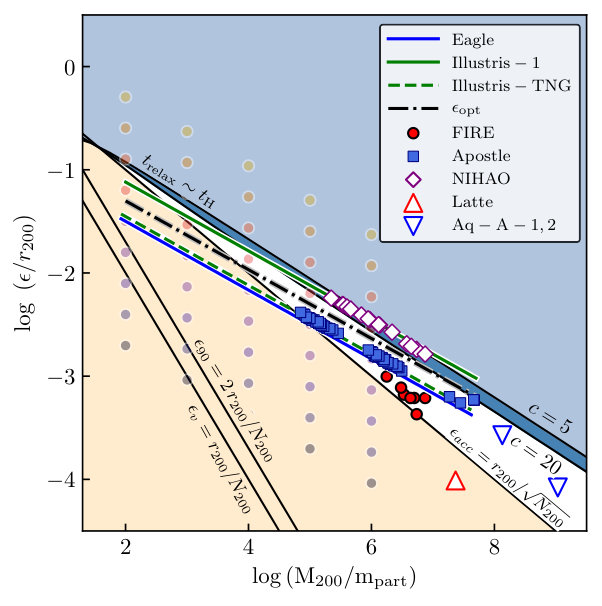 Figure 1
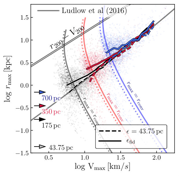 Figure 10
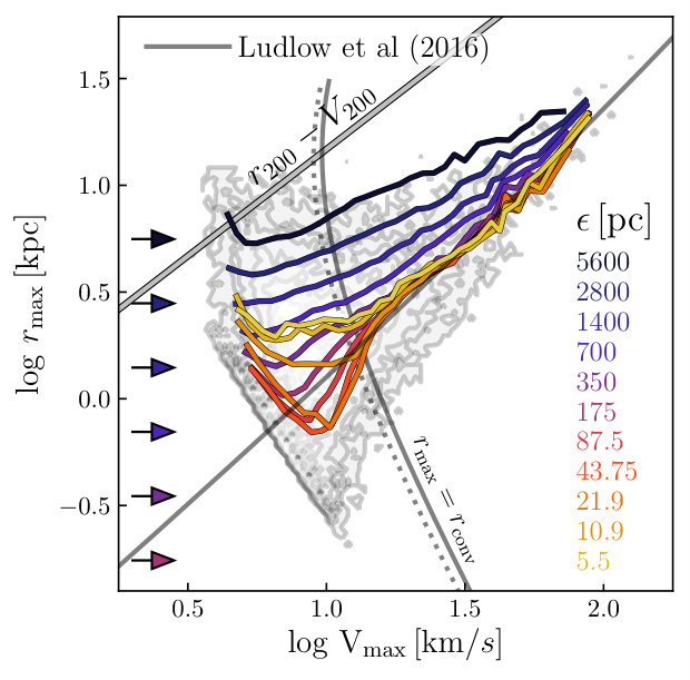 Figure 10
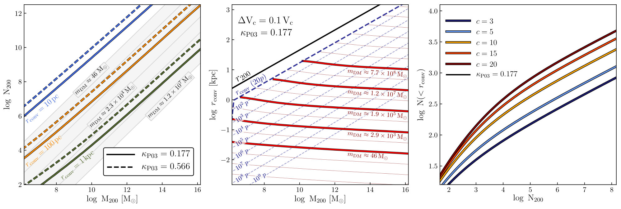 Figure 11
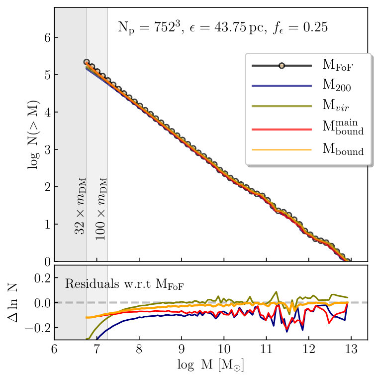 Figure 12
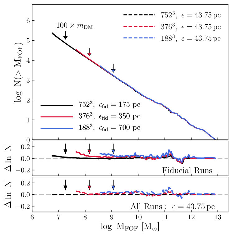 Figure 13
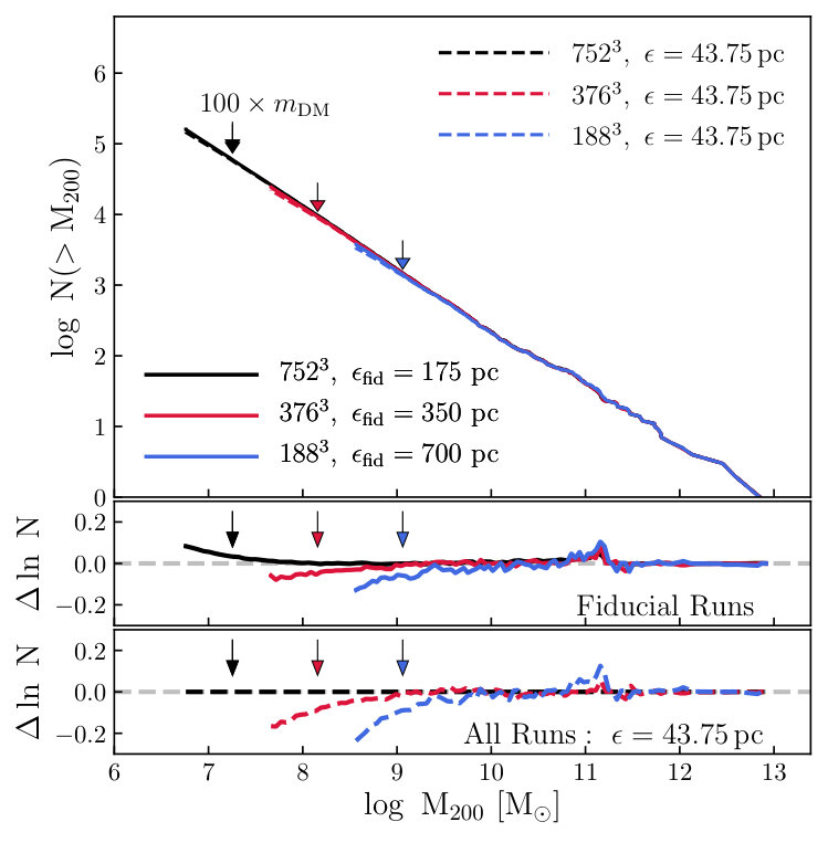 Figure 13
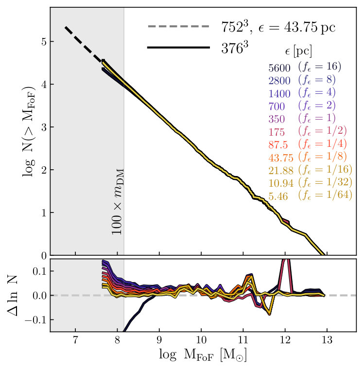 Figure 13
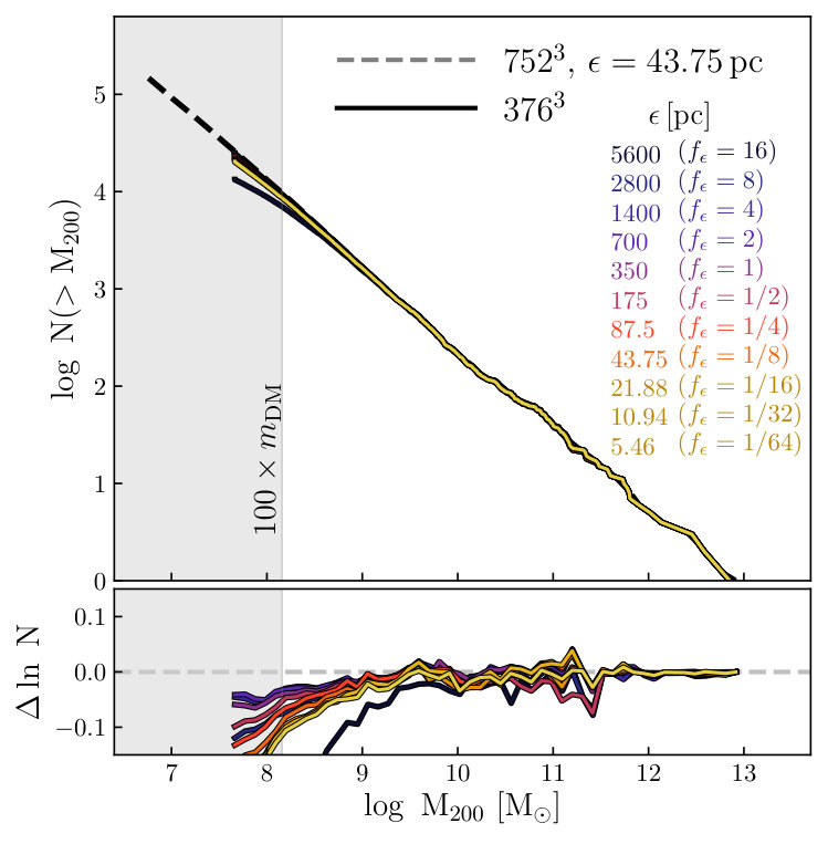 Figure 13
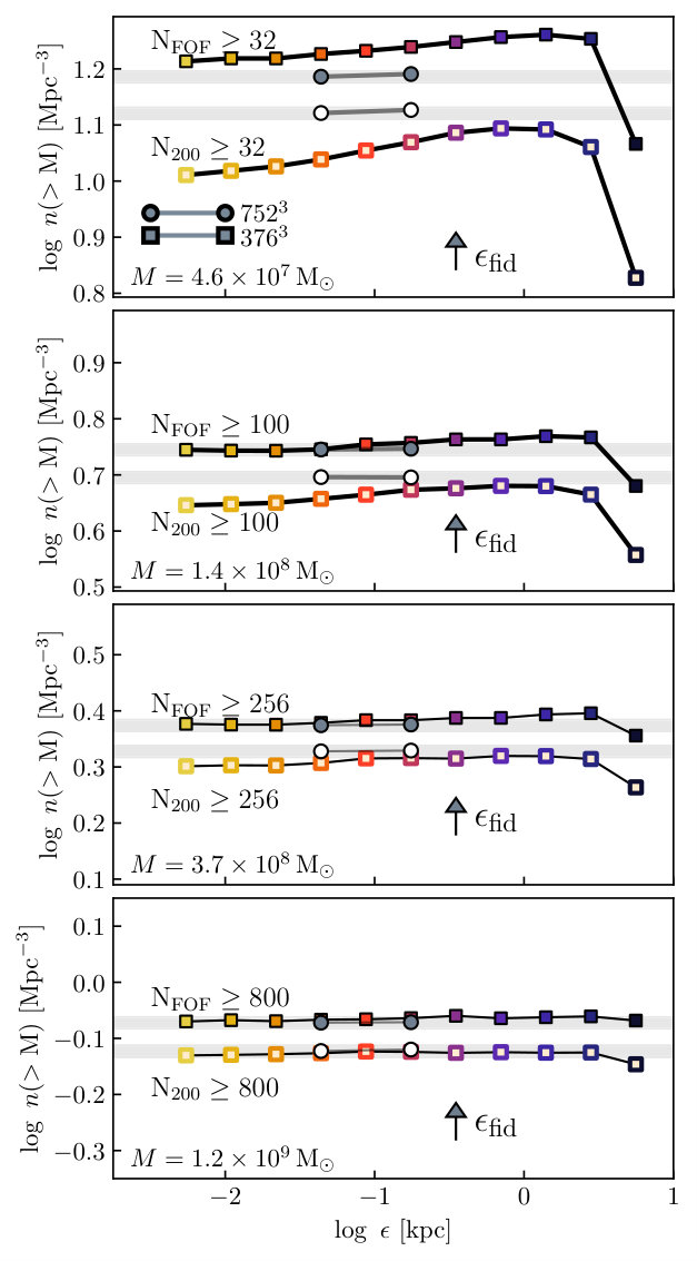 Figure 14
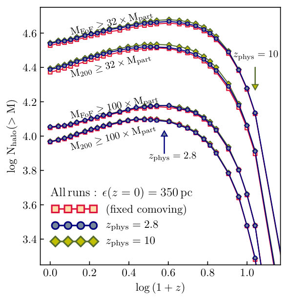 Figure 15
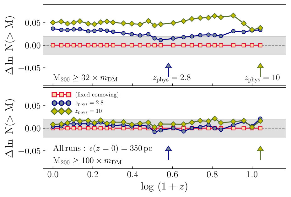 Figure 16
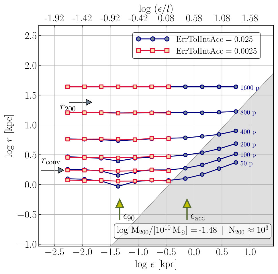 Figure 2
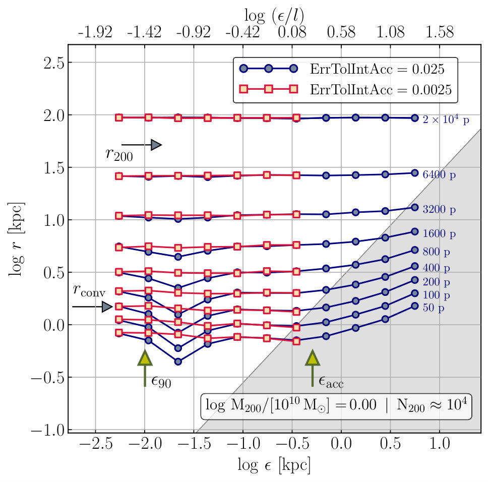 Figure 2
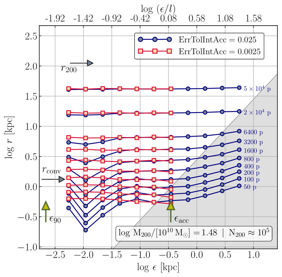 Figure 2
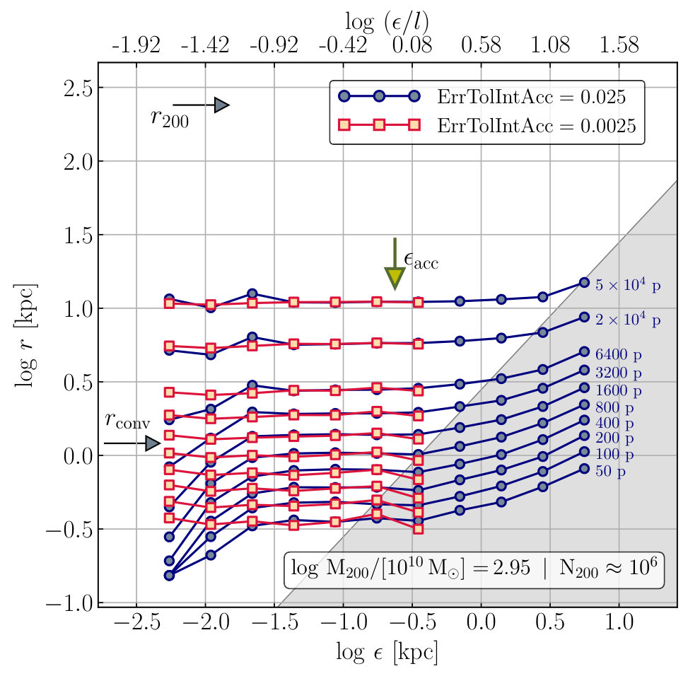 Figure 2
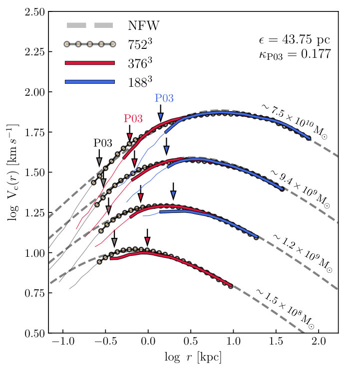 Figure 3
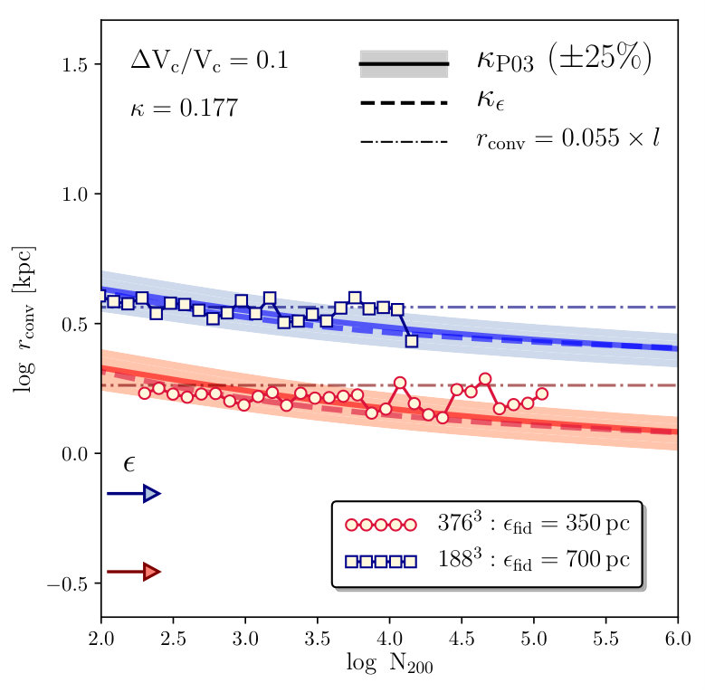 Figure 4
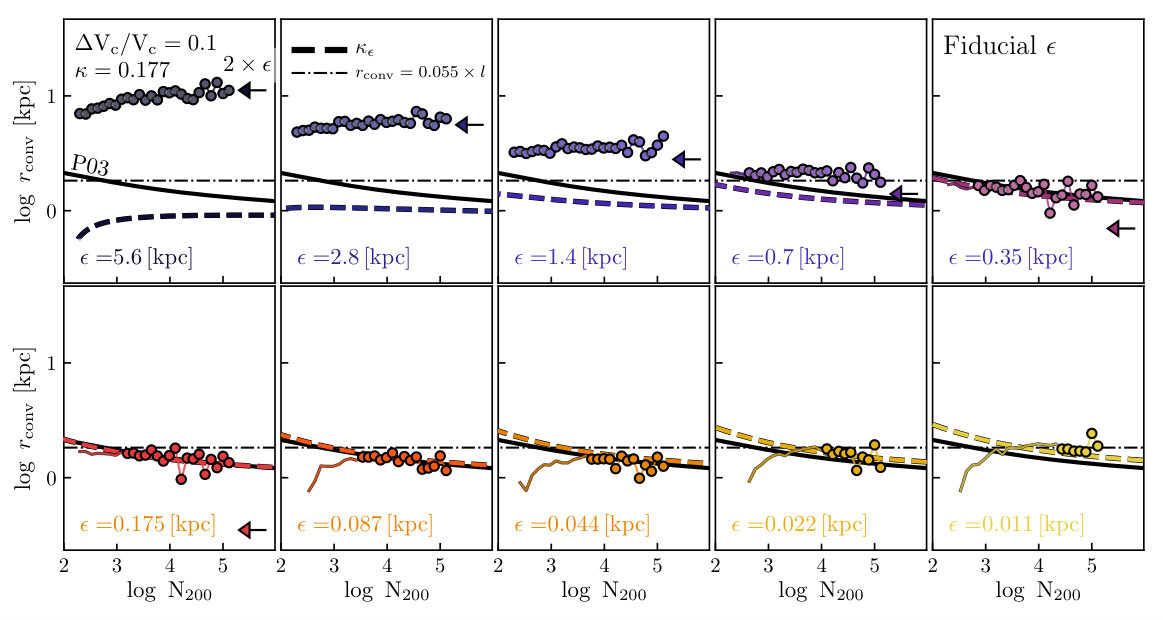 Figure 5
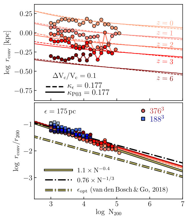 Figure 6
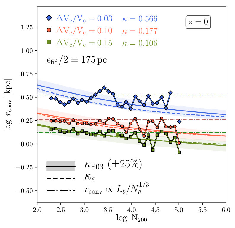 Figure 7
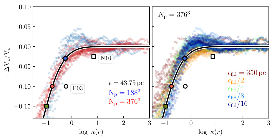 Figure 8
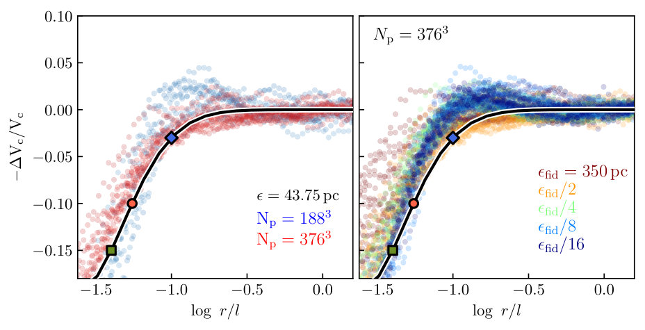 Figure 8
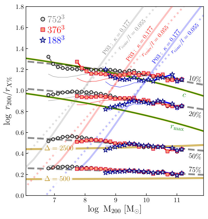 Figure 9
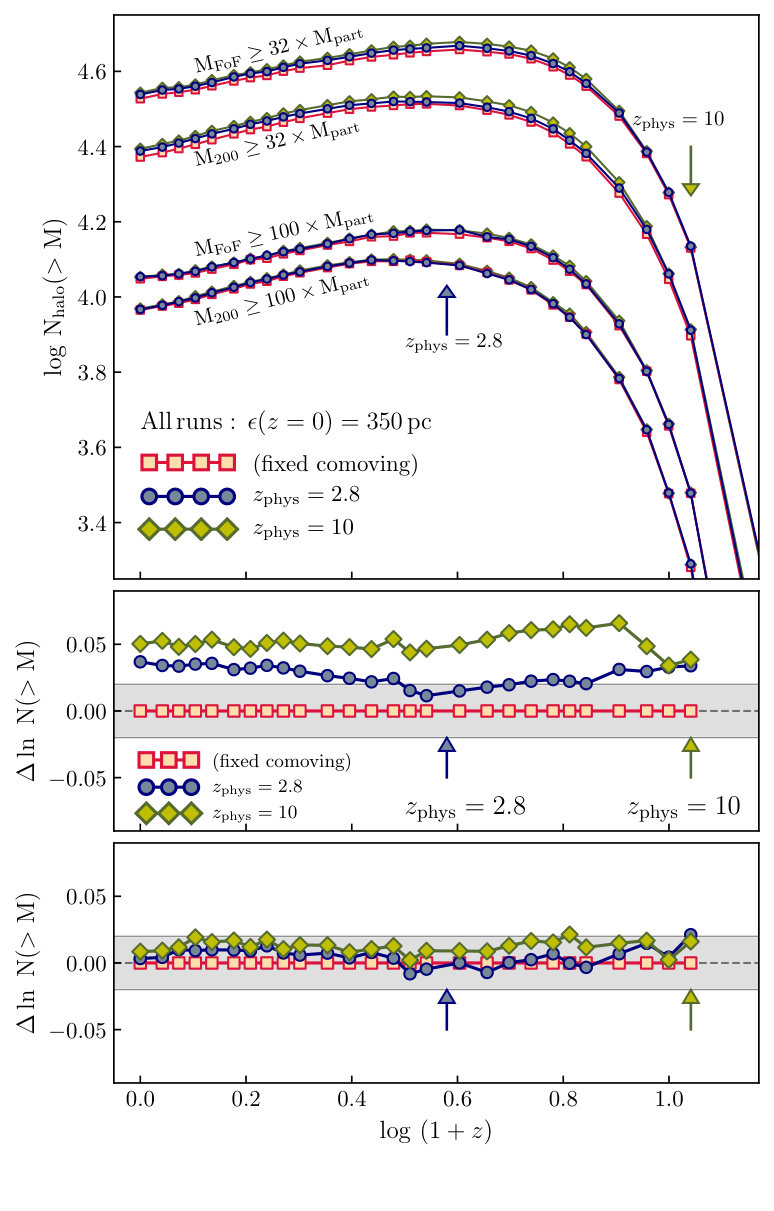 Figure 25
| Name | ErrTolIntAcc | ||||||||||
|---|---|---|---|---|---|---|---|---|---|---|---|
| [] | |||||||||||
| L0012N0752 | 1.8 | 7523 | 175.0 | 1.05 | 665.0 | 4.00 | 1.0000 | 0.025 | 2.8 | ||
| L0012N0752 | 1.8 | 7523 | 43.8 | 0.26 | 166.3 | 2.00 | 0.2500 | 0.010 | 2.8 | ||
| L0012N0376 | 14.4 | 3763 | 5600.0 | 16.84 | 2.1 | 64.01 | 16.0000 | 0.025 | 2.8 | ||
| L0012N0376 | 14.4 | 3763 | 2800.0 | 8.42 | 10.6 | 32.01 | 8.0000 | 0.025 | 2.8 | ||
| L0012N0376 | 14.4 | 3763 | 1400.0 | 4.21 | 5320.0 | 16.00 | 4.0000 | 0.025 | 2.8 | ||
| L0012N0376 | 14.4 | 3763 | 700.0 | 2.11 | 2660.0 | 8.00 | 2.0000 | 0.025 | 2.8 | ||
| L0012N0376 | 14.4 | 3763 | 350.0 | 1.05 | 1330.0 | 4.00 | 1.0000 | 0.025, 0.0025 | 2.8 | ||
| L0012N0376 | 14.4 | 3763 | 175.0 | 0.53 | 665.0 | 2.00 | 0.5000 | 0.025, 0.0025 | 2.8 | ||
| L0012N0376 | 14.4 | 3763 | 87.5 | 0.26 | 332.5 | 1.00 | 0.2500 | 0.025, 0.0025 | 2.8 | ||
| L0012N0376 | 14.4 | 3763 | 43.8 | 0.13 | 166.3 | 0.50 | 0.1250 | 0.025, 0.0025 | 2.8 | ||
| L0012N0376 | 14.4 | 3763 | 21.9 | 0.07 | 83.13 | 0.25 | 0.0625 | 0.025, 0.0025 | 2.8 | ||
| L0012N0376 | 14.4 | 3763 | 10.9 | 0.03 | 41.6 | 0.13 | 0.0313 | 0.025, 0.0025 | 2.8 | ||
| L0012N0376 | 14.4 | 3763 | 5.5 | 0.02 | 20.8 | 0.06 | 0.0156 | 0.025, 0.0025 | 2.8 | ||
| L0012N0376 | 14.4 | 3763 | 350.0 | 1.05 | 350.0 | 1.05 | 1.0000 | 0.025 | 0.0 | ||
| L0012N0376 | 14.4 | 3763 | 350.0 | 1.05 | 2609.2 | 8.09 | 1.0000 | 0.025 | 10.0 | ||
| L0012N0188 | 115.0 | 1883 | 700.0 | 1.05 | 2660.0 | 4.00 | 1.0000 | 0.025 | 2.8 | ||
| L0012N0188 | 115.0 | 1883 | 350.0 | 0.53 | 1330.0 | 2.00 | 0.5000 | 0.025 | 2.8 | ||
| L0012N0188 | 115.0 | 1883 | 175.0 | 0.26 | 665.0 | 1.00 | 0.2500 | 0.025 | 2.8 | ||
| L0012N0188 | 115.0 | 1883 | 87.5 | 0.13 | 332.5 | 0.50 | 0.1250 | 0.025 | 2.8 | ||
| L0012N0188 | 115.0 | 1883 | 43.8 | 0.07 | 166.3 | 0.20 | 0.0625 | 0.025 | 2.8 | ||
| L0012N0188 | 115.0 | 1883 | 21.9 | 0.03 | 83.13 | 0.13 | 0.0313 | 0.025 | 2.8 |
Peer Reviews
No public reviews on file for this paper yet. If you reviewed it on a platform where reviews are public (OpenReview, ICLR, NeurIPS, ICML), you can paste yours below so the community can read it here.
Videos
No videos yet. Explain this paper in a talk, walkthrough, or lecture? Add one.
Numerical convergence of simulations of galaxy formation: the abundance and internal structure of cold dark matter haloes
Aaron D. Ludlow1,⋆, Joop Schaye2 & Richard Bower3
1International Centre for Radio Astronomy Research, University of Western Australia, 35 Stirling Highway, Crawley,
Western Australia, 6009, Australia
2Leiden Observatory, Leiden University, PO Box 9513, 2300 RA Leiden, the Netherlands
3Institute for Computational Cosmology, Department of Physics, Durham University, Durham DH1 3LE, U.K.
Abstract
We study the impact of numerical parameters on the properties of cold dark matter haloes formed in collisionless cosmological simulations. We quantify convergence in the median spherically-averaged circular velocity profiles for haloes of widely varying particle number, as well as in the statistics of their structural scaling relations and mass functions. In agreement with prior work focused on single haloes, our results suggest that cosmological simulations yield robust halo properties for a wide range of gravitational softening parameters, , provided: 1) is not larger than a “convergence radius”, , which is dictated by 2-body relaxation and determined by particle number, and 2) a sufficient number of timesteps are taken to accurately resolve particle orbits with short dynamical times. Provided these conditions are met, median circular velocity profiles converge to within per cent for radii beyond which the local 2-body relaxation timescale exceeds the Hubble time by a factor \kappa\equiv t_{\rm relax}/t_{\rm H}\lower 2.15277pt\hbox{;\buildrel>\over{\sim};}0.177, with better convergence attained for higher . We provide analytic estimates of that build on previous attempts in two ways: first, by highlighting its explicit (but weak) softening-dependence and, second, by providing a simpler criterion in which is determined entirely by the mean inter-particle spacing, ; for example, better than per cent convergence in circular velocity for r\lower 2.15277pt\hbox{;\buildrel>\over{\sim};}0.05\,l. We show how these analytic criteria can be used to assess convergence in structural scaling relations for dark matter haloes as a function of their mass or maximum circular speed.
keywords:
cosmology: dark matter, theory – galaxies: formation – methods: numerical
11footnotetext: E-mail: [email protected]
1 Introduction
Cosmological simulations have become an essential component of astronomical science. Simulations of collisionless cold dark matter (CDM), in particular, have matured to a point where both the statistical properties of large-scale structure, as well as the highly non-linear structure of dark matter haloes are largely agreed upon, even between groups employing widely varying simulation or analysis methods. Among these are: the topology of large-scale structure (e.g. Gott et al., 1987; James et al., 2007; Blake et al., 2014); the matter power spectrum (e.g. Smith et al., 2003); the clustering (e.g. Kaiser, 1984; White et al., 1987; Poole et al., 2015; Tinker et al., 2010), mass function (e.g. Jenkins et al., 2001; Reed et al., 2003; Tinker et al., 2008; Despali et al., 2016) and shapes (e.g. Allgood et al., 2006; Despali et al., 2014; Vera-Ciro et al., 2014; Vega-Ferrero et al., 2017) of dark matter haloes; their spherically averaged mass profiles (e.g. Navarro et al., 1996, 1997; Bullock et al., 2001; Ludlow et al., 2013; Dutton & Macciò, 2014); mass assembly histories (e.g. van den Bosch, 2002; Zhao et al., 2009; Correa et al., 2015a, b) and the mass function and radial distribution of their substructure populations (e.g. Ghigna et al., 1998; Stoehr et al., 2003; Gao et al., 2004; Springel et al., 2008).
The radial mass profile of dark matter haloes is a particularly important and robust prediction of N-body simulations. For relaxed haloes it can be approximated by the NFW profile (Navarro et al., 1996, 1997), though slight deviations from this form have been reported extensively in the literature (e.g. Navarro et al., 2004; Ludlow et al., 2013; Dutton & Macciò, 2014; Ludlow & Angulo, 2017). The NFW profile has a central cusp where densities diverge as and a steep outer profile where tapers off as . In parametric form, the spherically averaged density profiles can be well approximated by
[TABLE]
where and are characteristic values of density and radius.
Agreement on these issues required pain-staking tests of numerical convergence that demanded repeatability of simulation results, regardless of the numerical methods employed or the numerical parameters adopted. A number of these studies led to the development of useful “convergence criteria” that can be used to disentangle aspects of simulations that are reliably modelled from those that may be affected by numerical artifact. These studies differ in the details, but uniformly agree that systematic convergence tests are necessary to validate the robustness of a particular numerical result. Numerical requirements for convergence in halo mass functions, for example, may differ substantially from those required for convergence in shapes, dynamics or mass profiles.
For collisionless CDM, once a cosmological model has been specified, only numerical parameters remain. The starting redshift and finite box size of simulations, for example, affect halo mass functions and clustering, but leave the internal properties of dark matter haloes largely unchanged (Knebe et al., 2009; Power & Knebe, 2006). Other parameters impose strict limits on spatial resolution, or otherwise alter the inner structure of haloes in non-trivial ways. Of particular importance are the gravitational force softening, (which prevents divergent pairwise forces and suppresses large-angle deflections), the integration timestep for the equations of motion, , and the particle mass resolution, .
Power et al. (2003, hereafter P03) provided a comprehensive survey of how these numerical parameters affect the internal structure of a simulated CDM halo. They conclude that convergence in mass profiles can be achieved for suitable choices of timestep, softening, particle number and force accuracy. For choices of softening that suppress discreteness effects, and for timesteps substantially shorter than the local dynamical time, circular velocity profiles converge to within \lower 2.15277pt\hbox{;\buildrel<\over{\sim};}10 per cent roughly at the radius enclosing a sufficient number of particles to ensure that the local 2-body relaxation time exceeds a Hubble time. Their tests led to the development of what is now a standard choice for the “optimal” softening for cosmological simulations, and to an empirical prescription for calculating the “convergence radius” of dark matter haloes. Their results – which we put to the test in subsequent sections – have been validated and extended by a number of follow-up studies (e.g. Diemand et al., 2004; Springel et al., 2008; Navarro et al., 2010; Gao et al., 2012).
Strictly speaking, the criteria laid out by P03 mainly apply to convergence in the circular velocity profiles, , of individual haloes, and may not apply to convergence in other quantities of interest, such as their shapes (Vera-Ciro et al., 2014), mass functions (e.g. Reed et al., 2003), to various aspects of their substructure distributions (e.g. Ghigna et al., 2000; Reed et al., 2005; Springel et al., 2008), or to population-averaged profiles of, for example, density or circular velocity. We focus on the latter in this paper.
P03 defined convergence empirically: the same simulation was repeated multiple times using different numerical parameters and the results were used to quantify the radial range over which remained insensitive to those choices. van den Bosch & Ogiya (2018) follow a different approach. Using a series of idealized numerical experiments, they argue that inappropriate choices for gravitational softening are detrimental to the evolution of substructure haloes and that, as a result, many state-of-the-art cosmological simulations are still subject to the classic “over-merging” problem (Moore et al., 1996). They additionally argue that discreteness-driven instabilities in subhaloes with \lower 2.15277pt\hbox{;\buildrel<\over{\sim};}10^{3} particles forbids a proper assessment of their evolution in strong tidal fields, limiting our ability to interpret convergence in their mass functions or internal structure.
In this paper, we interpret convergence in the median profiles of halos in terms of 2-body relaxation, which varies from system-to-system depending on the number of particles used to sample their mass profile. To do so, we carry out the same simulation several times but with different numbers of particles, allowing us to compare the same sub-population (i.e. those occupying a particular mass bin) at varying resolution. It is important to note, however, that 2-body scattering may not be the sole driver of relaxation in collisionless systems. Collective relaxation, for example, is a distinct process by which individual particle trajectories are altered repeatedly in response to large-scale and potentially long-lived fluctuations to the global potential (see e.g. Weinberg, 1993). This is neglected in simple analytic estimates of collisional relaxation rates, such as those presented in Section 3.2 (see also Chandrasekhar, 1943; Hénon, 1961; Cohn & Kulsrud, 1978), but may dominate when fluctuations are comparable to the size of the system under consideration. The fluctuations may be physical, or form as a result of discreteness-driven noise in collisionless -body simulations. Indeed, it has been argued that this process may give rise to artificial fragmentation that plagues traditional -body simulations of warm dark matter models, but appears to have measurable effects in CDM simulations as well (see, e.g., Power et al., 2016, and references therein).
Going beyond pure dark matter (DM), hydrodynamic simulations of galaxy formation are reaching new levels of maturity. The increase of computational resources and improved algorithms enable fully cosmological simulations of galaxy formation to be carried out; simulations that often resolve tens of thousands of individual galaxies in volumes approaching those required for cosmological studies. Notable among these are eagle (Schaye et al, 2015; Crain et al., 2015), Illustris (Vogelsberger et al., 2014a; Pillepich et al, 2018), Horizon-AGN (Dubois et al, 2014), and the Magneticum Pathfinder simulations (Dolag et al., 2016). Although sub-grid models in simulations such as these must be calibrated to reproduce a desired set of observables (for eagle, the galaxy stellar mass function and size-mass relation), many of their predictions have been ratified by observations making them a useful tool for interpreting observational data and for illuminating the complex physical processes that give rise to galaxy scaling relations.
As discussed by Schaye et al (2015), the need to calibrate subgrid models in simulations affects our ability to interpret numerical convergence, particularly when mass and spatial resolution are improved. Clearly convergence is a requirement for predictive power, but for a multi-scale process such as galaxy formation it should arguably be attained only after recalibration of the subgrid physics, thus allowing models to benefit from increased resolution by incorporating new, scale-dependent physical processes.
The convergence of hydrodynamic simulations is, in any event, poorly understood. It remains unclear, for example, how robust predictions of galaxy formation models are to small changes in the numerical parameters. To cite an example, Ludlow et al. (2019) recently pointed out that simulated galaxy sizes, quantified by their projected half-mass radii, grow over time as a result of spurious energy transfer between stellar and DM particles of unequal mass. The effect can be suppressed by adopting a stellar to DM particle mass ratio that is close to unity, even when other numerical and subgrid parameters are unchanged. We seek to further address these issues using a suite of simulations drawn from the eagle project. In this first paper we study the sensitivity of our simulations to numerical parameters when only dark matter is present, seeking to illuminate and clarify shortcomings of prior work. In a follow-up paper, we will address convergence in fully-hydrodynamical simulations using a well-calibrated galaxy formation model from the eagle project.
Our study is part of the eagle Project. All of our runs were carried out using the same simulation code and adopt the same “fiducial” numerical parameters as Schaye et al (2015), which we vary systematically from run-to-run. We concentrate our discussion primarily on gravitational softening and the impact of 2-body collisions on the spatial resolution of N-body simulations, but consider mass resolution and timestepping when necessary. Softening has been studied in great detail in the past two decades, but this has not led to a clear consensus on what constitutes an “optimal” softening length for a given simulation.
The remainder of the paper is organized as follows. In Section 2.1 we describe our simulation suite and the variation of numerical parameters, as well as halo finding techniques (Section 2.2). We provide simple analytic estimates of plausible bounds on gravitational softening in Section 3; we introduce the 2-body “convergence radius” in Section 3.2, highlighting its explicit dependence on softening. We then present our main results: the convergence of median circular velocity profiles is discussed in Section 4, followed by that of mass functions (Section 5). We summarize and conclude in Section 6.
2 Simulations
2.1 Simulation set-up
All runs were carried out in the same cubic periodic volume which was simulated repeatedly using different numbers of particles, , gravitational softening lengths, , and timestep size, . Each run adopted the set of “Planck” cosmological parameters used for eagle (Schaye et al, 2015; Planck Collaboration et al., 2014): ; ; ; ; . Here is the energy density of component expressed in units of the critical density, ; is Hubble’s constant; is the linear rms density fluctuation in 8 ; and is the primordial power spectral index. Initial conditions for each simulation were generated using second-order Lagrangian perturbation theory at (Jenkins, 2013), which is sufficiently high to ensure that all resolved modes are initially well within the linear regime. We sample the linear density field with , and equal-mass particles; the corresponding particle masses are , and . All simulations sample resolved modes using the same initial phases. For consistency we label each run in a way that encodes the box size and particle number, using the same nomenclature as Schaye et al (2015). For example, L0012N0376 corresponds to a run with and particles. The DM density field is evolved using the same version of P-gadget (Springel, 2005) employed for the eagle project.
It is common in the literature to refer to as the “spatial resolution” of a simulation, not surprisingly given its dimensions. For cosmological simulations of uniform mass resolution it is customary to adopt a gravitational softening length that is a fixed fraction of the (comoving) mean inter-particle separation,
[TABLE]
thus fixing the ratio . In eagle the softening parameter, initially fixed in comoving coordinates, reaches a maximum physical value at redshift , after which it remains constant in physical coordinates. For , and , this implies, for , while in co-moving coordinates for . We will hereafter refer to as the “fiducial” softening length regardless of mass resolution, and will vary away from this value by successive factors of two. For the “fiducial” softening length is ; for , and for . We further note that refers to the Plummer-equivalent softening length, which is related to the “spline” softening length used by P-gadget through
[TABLE]
To test the sensitivity of our results to changing , we have also carried out runs with (fixed co-moving at all ) and (fixed physical ). For convenience, we will sometimes reference softening parameters relative to the fiducial value, hence defining the relative softening length . Table 1 lists all of the relevant numerical parameters for our simulations.
2.2 Halo identification
We identify haloes in all of our simulations using the subfind (Springel et al., 2001) algorithm. subfind first links dark matter particles into friends-of-friends (FoF) groups before separating them into a number of self-bound “subhaloes”. Each FoF group contains a central or “main” subhalo that contains most of its mass, and a number of lower-mass substructures. For each FoF halo and its entire hierarchy of subhaloes subfind records a number of attributes, the most basic of which include its mass, (for FoF haloes), position (defined as the location of the particle with the minimum potential energy) and the magnitude and location of its peak circular speed, and . For FoF haloes (defined as “main” haloes in what follows), subfind also records other common mass definitions based on a variety of spherical overdensity (SO) boundaries: is the mass contained within a spherical region whose mean density is 200; encloses a mean density of , where is the redshift-dependent virial overdensity of Bryan & Norman (1998) ( for our adopted cosmology). Using as a starting-point all FoF particles in a given halo, subfind also computes its gravitationally-bound mass, , as well as the mass bound to each of its subhaloes. Each of these are common and sensible ways to define halo masses, which we compare in Section 5.2. Note that the virial mass of a halo implicitly defines its virial radius, , and corresponding circular velocity, : for an overdensity , for example, , and .
In addition to halo properties, subfind also records lists of particles belonging to each halo (which include all bound as well as unbound particles within ), which we use to calculate their spherically-averaged enclosed mass profiles, . Note that all particles contribute to , and not only those that subfind deems bound to the halo. This choice precludes any subtle dependence of our results on subfind’s unbinding algorithm. We construct these profiles for all main haloes in 50 equally-spaced logarithmic bins spanning which we then use to build median circular velocity profiles, , as a function of halo mass, and various other structural scaling relations. Note that all particles are used to calculate , and not just those deemed bound to the main halo by subfind. The results presented in the following sections are obtained using these spherically-averaged profiles, and the halo masses returned by subfind.
Assessing convergence in properties of substructure is challenging (see van den Bosch & Ogiya, 2018; van den Bosch et al., 2018, for a recent in depth analysis). For that reason, we will focus our analysis on isolated haloes expected to host central galaxies in hydrodynamic runs.
3 Analytic expectations
3.1 Preliminaries: limits on gravitational softening
Softening gravitational forces in N-body simulations has distinct advantages. In particular, it suppresses large-angle deflections due to (artificial) 2-body scattering, thereby permitting the use of low-order orbit integration schemes. This substantially decreases wall-clock times required for a given N-body problem. There are, however, drawbacks: when is small shot noise in the particle load can result in large near-neighbor forces, or when large, to systematic suppression of inter-particle forces. Both effects can jeopardize the results of N-body simulations and the optimal choice of gravitational softening should provide a compromise between the two.
The finite particle mass and limited force resolution inherent to particle-based simulations can give rise to adverse discreteness effects if is not properly chosen, and the debate over what constitutes a wise choice persists. Some studies, designed specifically to annotate discreteness-driven noise in simulations, suggest a safe lower limit to softening of \epsilon/l\lower 2.15277pt\hbox{;\buildrel>\over{\sim};}1-2 (e.g. Melott et al., 1997; Power et al., 2016). This is supported by others who argue that various two-point statistics of the DM density field are not converged on scales \lower 2.15277pt\hbox{;\buildrel<\over{\sim};}l (Splinter et al., 1998). It is important to note, however, that discreteness noise does not propagate from the small scales where it is introduced to larger ones, being typically confined to scales of order to (Romeo et al., 2008).
Whether simulations are trustworthy below scales remains a matter of debate. Claims above to the contrary are often based on particular cases: cold, plane-symmetric collapse and simulations with truncated linear power spectra give rise to spurious clustering as a result of discreteness-driven relaxation. The effect is prominent in simulations of hot and warm DM models (e.g. Avila-Reese et al., 2001; Bode et al., 2001; Knebe et al., 2003), where counterfeit haloes form as a result of anisotropic force errors occurring during the initial phases of filamentary collapse (Hahn et al., 2013). These haloes follow a spatial pattern that reflects the Lagrangian inter-particle spacing, but remain prominent in warm DM simulations that adopt isotropic softening lengths of order (Power et al., 2016). Better success at stifling these haloes has been achieved using adaptive, anisotropic softening lengths (Hobbs et al., 2016) or alternatives to traditional N-body methods (Angulo et al., 2013).
Power et al. (2016) argue that spurious haloes are also present in CDM models, but their prevalence has not been quantified due to difficulties disentangling them from “genuine” ones. Using simulations of hot DM models, Wang & White (2007) showed that spurious structures dominate the halo mass function on scales below a limiting mass given by
[TABLE]
where is the mean matter density and is the wavenumber at which the dimensionless matter power spectrum, , reaches a maximum. Assuming , we can write eq. 4 in terms of the maximum comoving size of spurious haloes:
[TABLE]
where is the Nyquist frequency, and in the second expression we have used and . For CDM models, finite resolution suggests that , implying (assuming eq. 4 remains valid in this regime).
It is useful to compare to the comoving virial radius of the lowest-mass haloes resolved in cosmological CDM simulations. Noting that and , this can be written
[TABLE]
Note, for CDM, when , suggesting spurious haloes are negligible for models in which increases to arbitrarily small scales. For models with suppressed small-scale power, on the other hand, spurious haloes may dominate at low masses. For example, r_{\rm lim}\lower 2.15277pt\hbox{;\buildrel>\over{\sim};}l provided the Power spectrum “turn over” is resolved with \lower 2.15277pt\hbox{;\buildrel>\over{\sim};}54 resolution elements.
To avoid biasing gravitational collapse at the resolution limit of CDM simulations, the comoving softening length should therefore remain smaller than the comoving virial radius of the lowest-mass haloes that can be resolved. Indeed, Lukić et al. (2007) and Power et al. (2016) showed that CDM halo mass functions are substantially suppressed on scales below which the softening length exceeds the halo virial radius. For a conservative resolution limit of , eq. 6 suggests that should remain smaller than about one third of the mean inter-particle spacing; for , \epsilon/l\lower 2.15277pt\hbox{;\buildrel<\over{\sim};}0.2 is required.
Most recent large-scale simulations adopt softening lengths substantially smaller than these limits, but large enough to ensure that the lowest-mass haloes resolved by the simulation remain approximately collisionless***No haloes are truly collisionless in particle-based simulations. We use the phrase here to refer to haloes in which collisional dynamics driven by 2-body interactions remain small compared to those dictated by the global potential. at all times. One such criterion demands that the specific binding energy of low-mass haloes, , remains larger than the binding energy of two DM particles separated by : . The condition imposes a lower limit on of
[TABLE]
Eq. 7 can also be expressed , where we have used the fact that . This is comparable to the softening length required to suppress large-angle deflections during close encounters, given by , where is the impact parameter giving rise to deflections (Binney & Tremaine, 1987) and is the typical speed of particles at distance . This condition therefore requires \epsilon_{90}\lower 2.15277pt\hbox{;\buildrel>\over{\sim};}2\,r_{200}/N_{200}, a factor of 2 larger than . Suppressing large accelerations during to close encounters results in stricter limits on softening (see P03). For example, requiring that the maximum stochastic acceleration due to close encounters, , remains smaller than the minimum mean-field acceleration across the entire halo, , imposes a lower limit of \epsilon_{\rm acc}\lower 2.15277pt\hbox{;\buildrel>\over{\sim};}r_{200}/\sqrt{N_{200}}.
For eq. 7 implies a lower limit of \epsilon/l\lower 2.15277pt\hbox{;\buildrel>\over{\sim};}0.01, comparable to values adopted for essentially all recent large-scale simulations projects. The Bolshoi simulation (Klypin et al., 2011), for example, had a force resolution of , while the Multi-dark simulations (Klypin et al., 2016) adopted (Plummer equivalent); the Millennium (Springel et al., 2005), Millennium-II (Boylan-Kolchin et al., 2009) and Millennium-XXL (Angulo et al., 2012) each used ; for DUES FUR (Alimi et al., 2012); for Copernicus Complexio (Hellwing et al., 2016). Cosmological hydrodynamical simulations use comparable values of softening: as mentioned above, eagle adopted a physical softening length of ( in co-moving coordinates at ), while Illustris-TNG used maximum physical value of (Springel et al., 2018). All values above are quoted as physical softening lengths at , unless stated otherwise. We will see in Section 3.2 that the median circular velocity profiles of haloes in collisionless cosmological simulations are affected by 2-body scattering at radii that generally exceed these softening lengths. For example, converges to better than 10 per cent a radii r\lower 2.15277pt\hbox{;\buildrel>\over{\sim};}0.055\times l, and to better than 3 per cent for r\lower 2.15277pt\hbox{;\buildrel>\over{\sim};}0.10\times l (section 4.3). In all of these runs, softening is unlikely to compromise the mass profiles of haloes on scales not already influenced by 2-body relaxation.
As mentioned above, the “optimal” softening, , for a given simulation is the one that balances large force errors due to shot noise with biases resulting from large departures from the Newtonian force law. Merritt (1996) suggested that should be chosen to minimize the average square error in force evaluations relative to what is expected from an equivalent smooth matter distribution. A drawback of this approach is that depends not only on the mass distribution under consideration – which is not generally known a priori – but also on the number of particles in the system, . Dehnen (2001), for example, found that the optimal softening for a Hernquist (1990) halo is roughly , where is its scale radius. van den Bosch & Ogiya (2018) find that , a result obtained by studying the stability of the central cusp of an isolated NFW halo ( and ) to long-term secular evolution (); the scaling with is motivated by the work of van Kampen (2000). We will see in Section 5.3 that this is sufficiently small to avoid compromising the spatial resolution in halo centres in cosmological simulations using equal-mass particles. In our study, we consider a broad range of softening lengths, spanning to .
Figure 1 compares the softening lengths used in a number of recent state-of-the-art simulations, and shows for comparison the characteristic values , and mentioned above. Note that, in all cases, is expressed in units of the virial radius, , and plotted as a function of .
In summary, a number of previous studies suggest that there can be considerable errors affecting the results of N-body simulations on scales \lower 2.15277pt\hbox{;\buildrel<\over{\sim};}l (e.g. Peebles et al., 1989; Melott et al., 1997; Splinter et al., 1998; Romeo et al., 2008). These may be driven by discreteness-noise (e.g. Power et al., 2016) or errors that affect phases of the Fourier component on such scales (see, e.g., Melott, 2007). Their severity, however, depends on the linear power spectrum adopted, or the type of simulation or statistic studied. Regardless, this underscores the need to establish independent convergence criteria for all results obtained from simulations, and to abstain from the common view that the softening length, or particle mass, represent meaningful “resolution limits”.
3.2 2-Body relaxation and the convergence radius
3.2.1 The relaxation timescale
It is important to emphasize that softening pair-wise forces does not necessarily increase 2-body relaxation times, which generally impose stricter constraints on the spatial resolution of N-body simulations. To see why, consider the cumulative effect of 2-body interactions incurred by a test particle as it crosses an -particle system with surface mass density . Following Binney & Tremaine (1987) (see also Huang et al., 1993; Farouki & Salpeter, 1982), we assume that any one encounter induces a small velocity perturbation perpendicular to the particle’s direction of motion, but leaves its trajectory unchanged. The perturbation due to a single encounter can be expressed
[TABLE]
where is the impact parameter and the (Plummer) softening length. In a single crossing, the test particle will experience such collisions with impact parameters spanning to . Integrating the square velocity change over all such encounters yields
[TABLE]
where and are, respectively, the minimum and maximum impact parameters, and we have assumed a typical velocity .
The relaxation time can be defined in terms of the number of orbits a test particle must execute in order to lose memory of its initial trajectory, i.e. . In the limit , eq. 9 implies
[TABLE]
where is the local orbital time, and we have assumed and . Eq. 10 is comparable to the classic relaxation time calculated by Binney & Tremaine (1987) for Keplerian forces, and depends only on the enclosed number of particles. Note that for a narrow range of impact parameter, , eq. 10 implies : fixed intervals of therefore contribute equally to relaxation, which is sensitive to both close and distant encounters. As a result, softening forces on small scales does little to prolong relaxation, which is primarily driven by large numbers of distant perturbers.
What is the appropriate choice of for haloes in cosmological simulations? If is chosen in order to suppress large-angle deflections, then the assumption may need revision. Indeed, for a Plummer potential there is a well-defined impact parameter†††This can be seen by maximizing the radial gradient of a Plummer force law and solving for . The minimum impact parameter obtained this way is slightly smaller than that which maximizes the velocity perturbation in eq. 8, which occurs at ., , for which the perpendicular pair-wise force between particles is maximized, tending to zero for both larger and smaller . Inserting this into eq. 9, and assuming , we obtain
[TABLE]
where the last two steps are valid provided . Note that eq. 13 depends logarithmically on , and is equivalent to eq. 10 if and . This confirms our expectation that softened forces give rise to modest changes in , even for very small values of the softening length (see also, e.g., Huang et al., 1993; Theis, 1998; Dehnen, 2001; Diemand et al., 2004). We will test this explicitly in Section 4.3.
3.2.2 The convergence radius
Collisional relaxation imposes a lower limit on the spatial resolution of N-body simulations that is typically larger than the limits on gravitational softening outlined in the previous section. Based on an extensive suite of simulations of individual Milky Way-mass haloes, P03 concluded that convergence is obtained at radii that enclose a sufficient number of particles so that the local two-body relaxation timescale is comparable to or longer than a Hubble time, , where is the circular orbital time at . The “convergence radius”, , implied by eq. 10 can thus be approximated by the solution to
[TABLE]
where is the mean internal density enclosing particles. We can rewrite eq. 14 in order to incorporate its explicit dependence on softening implied by eq. 11, resulting in
[TABLE]
Note that we have used subscripts on eqs. 14 and 15 in order to distinguish the P03 convergence radius from our softening-dependent estimate above, a convention we retain throughout the paper. Either equation, however, can be used to estimate once an empirical relationship between and “convergence” has been determined from simulations. P03 found that circular velocity profiles converge to better than per cent provided \kappa_{\rm P03}\lower 2.15277pt\hbox{;\buildrel>\over{\sim};}0.6. Navarro et al. (2010, hereafter N10) showed that better convergence can be obtained for larger values of ; at , for example, profiles converge to per cent. We follow P03 and N10 and quantify convergence in circular velocity profiles using , where and are the median profiles for haloes of fixed mass in our low- and highest-resolution simulations, respectively.
3.2.3 A simpler convergence criterion
As a useful approximation, we can rewrite the convergence radius implied by eq. 14 as
[TABLE]
where and ; these quantities depend weakly on concentration and , but also on . To illustrate, we set and solve eq. 14 assuming an NFW mass profile to determine for a range of concentrations and . We find that, for , varies by a factor \lower 2.15277pt\hbox{;\buildrel<\over{\sim};}2.4 for and \lower 2.15277pt\hbox{;\buildrel<\over{\sim};}1.9 for . Neglecting this weak dependence, eq. 16 implies that the ratio is approximately independent of mass and that, to first order, . As a result, haloes of a given will be “converged” roughly to a fixed fraction of their virial radii regardless of mass.
We can use these finding to cast eq. 16 into convenient forms that depend only on particle mass, or mean inter-particle spacing:
[TABLE]
where we have used the fact that ; is the mean inter-particle spacing in physical units. The latter result, eq. 18, implies that the ratio should be largely independent of redshift, halo mass and particle mass; the convergence radius is simply a fixed fraction of the mean inter-particle spacing. We will test these scalings explicitly in later sections.
Figure 1 plots (for ; thick black lines) for NFW profiles with and , representative of the vast majority of DM haloes that form in typical cosmological simulations. Due to the weak dependence of on , these curves are only slightly steeper than . As a result, adopting a fixed softening parameter for cosmological simulations with uniform mass resolution will not necessarily compromise spatial resolution at any mass scale. Take for example the solid blue line in Figure 1, which plots adopted for the eagle simulation. Here, is smaller than by more than a factor of 2 at all relevant halo masses (but will eventually exceed at very large ).
4 Median mass profiles
The most comprehensive attempt to establish the impact of numerical parameters on halo mass profiles has been the work of P03. Their results imply that, provided timestep size, softening and starting redshift are wisely chosen, particle number is the primary factor determining convergence.
One limitation of the work carried out by P03 and N10 is that they were based on simulations of a single dark matter halo that was resolved with at least particles, over 300 times that of the poorest resolved systems in typical cosmological runs. Can the conclusions of P03 be extrapolated to haloes with particles, or fewer? Is the P03 radial convergence criterion valid for stacked mass profiles, or for haloes whose masses differ substantially from ? We devote this section to addressing these questions.
4.1 Integration accuracy
The central regions of dark matter haloes are difficult to simulate due to their high densities, which reach many orders of magnitude above the cosmic mean. Crossing times there are to implying that thousands of orbits per particle must be integrated to ensure accuracy and reliability. Adding to this, haloes are not smooth and integration errors may accumulate during close encounters between particles. To prevent this, integration must be carried out with a minimum (but a priori unknown) level of precision. In gadget, particles take adaptive timesteps of length , where is the magnitude of the local acceleration, and is a parameter that allows some additional control over the step size. Clearly smaller timesteps are required when is small. In the gadget parameter file, is referred to as and takes on a default value of 0.025.
Figure 2 plots the average enclosed mass profiles of haloes drawn from our run, and highlights the importance of accurate integration. Panels correspond to different mass bins, which were selected so that (from top left to bottom right) , , and . The curves show the radii, , enclosing a given number of particles (indicated to the right of each curve) and are plotted as a function of the gravitational softening, . As a guide, the virial radius for each mass bin is indicated by the arrow on the left side of each panel. Connected (blue) circles show results for gadget ’s default integration accuracy parameter, .
For comparison, the vertical green arrows in each panel mark two estimates of minimum softening needed to suppress discreteness effects. The first, , ensures that the maximum stochastic acceleration felt by a particle () remains smaller than the minimum mean field acceleration of the halo (). The other, , is less restrictive and is required to prevent large-angle deflections during two-body encounters.
There are a couple points to note in this figure. First, central densities are noticeably suppressed for radii smaller than the “spline” softening length, i.e. r\lower 2.15277pt\hbox{;\buildrel<\over{\sim};}\epsilon_{\rm sp}=2.8\times\epsilon (in gadget , pairwise forces become exactly Newtonian for separations larger than ). This can be seen by noting that all radii appear to increase slightly once they cross into the grey shaded region, which delineates . Spatial resolution is clearly compromised at all radii \lower 2.15277pt\hbox{;\buildrel<\over{\sim};}\epsilon_{\rm sp}. More interestingly, however, the central regions of haloes show a clear increase in central density (i.e. the blue lines curve downward) when the softening parameter is reduced below a particular value. The value of at which this occurs depends on particle number, with more massive systems exhibiting symptoms at smaller . Note too that further reducing does not result in a denser centre: for very small , densities are again reduced. The asymptotic central density therefore depends non-monotonically on , suggesting a numerical origin.
The connected (red) squares show, for a subset of , the same results but for a series of runs in which was reduced from 0.025 to 0.0025 (this increases the total number of timesteps by a factor of roughly ). These curves are clearly flatter, suggesting that halo mass profiles are robust to changes in softening across a wide range of masses provided: a) is sufficiently small so that r\lower 2.15277pt\hbox{;\buildrel>\over{\sim};}\epsilon_{\rm sp}, and b) care is taken to ensure particle orbits are resolved with a sufficient number of timesteps. For the remainder of the paper, all results from runs for which were carried out with ErrTolIntAcc=0.0025, unless stated otherwise.
These results are qualitatively consistent with those of P03, but differ in the details. These authors report that gadget runs with fixed timestep developed artificially dense “cuspy” centres, where resolution is poor. Based on this, they argue for an -dependent adaptive timestepping criterion, , where . This is the same criterion adopted for our runs, but with a considerably larger value of , perhaps due to the much smaller softening parameters tested in our study. This may indicate the need for a timestepping criterion with a stronger dependence on . We defer this task to future work.
Provided a sufficient number of timesteps are taken, none of our runs appear to be adversely affected by being too small. Indeed, enclosed mass profiles appear stable at all r\lower 2.15277pt\hbox{;\buildrel>\over{\sim};}\epsilon even when \epsilon\lower 2.15277pt\hbox{;\buildrel<\over{\sim};}\epsilon_{90}, suggesting that hard scattering does not unduly influence the innermost structure of DM haloes, at least for the values of tested here. This may be because such scattering events are sufficiently rare (occurring with a cross-section proportional to ) that their cumulative effects are dynamically unimportant across a Hubble time. Averaged over much longer timescales, scattering-induced cores do develop in idealized simulations of isolated NFW haloes (see, for example, Figure 6 of van den Bosch & Ogiya 2018, who study the secular evolution of an NFW halo for Gyr).
These results suggest that the median mass profiles of dark matter haloes are remarkably robust to changes in gravitational softening provided it is not so large that it compromises enclosed masses. This is true even for haloes containing as few as particles, and for radii enclosing as few as . This does not, however, imply numerical convergence. Indeed, provided other numerical parameters are carefully chosen, 2-body relaxation places much stronger constraints on convergence (P03), and dense haloes centres – which occupy only a small fraction of their total mass and volume – are highly susceptible to low particle number. The systematic effects of 2-body scattering on the innermost mass profiles of dark matter haloes must therefore be carefully considered when seeking to quantify numerical convergence. As discussed above, a useful tactic for separating converged from unconverged parts of a halo is to identify the radius at which the collisional relaxation time is some multiple of a Hubble time (P03). We turn our attention to this in the following subsections.
4.2 Median circular velocity profiles
Figure 3 shows the median circular velocity profiles of haloes in four separate mass bins and at three different resolutions. Grey dashed lines show NFW fits to the profiles of haloes in our run (grey lines and circles). Because these curves agree well with the simulated profiles over a large radial range, we can use them to estimate the convergence radius by identifying the point at which the simulated profiles first dip below the theoretical ones by a certain amount. Thick lines (or points in the case of ) cover radii for which departs from dashed lines by less than 10 per cent; thin lines extend to radii enclosing particles.
Note that measured convergence radii are, for a given resolution, only weakly dependent on halo mass (the thick segments or points end at similar radii for a given set of curves). Haloes in our run, for example, have convergence radii that differ by at most 30 per cent across the entire mass range plotted (which corresponds to a factor of in and in ), and the difference is similar for the other resolutions. Two haloes with the same total number of particles therefore have very different convergence radii depending on their mass. For example, a halo of mass in our 7523 run has a measured convergence radius of , whereas haloes in our 1883 run–resolved with the same number of particles–, about a factor of 6 larger.
This scaling is indeed expected from eq. 16. Neglecting the weak dependence of concentration on halo mass, two haloes with the same number of particles identified in simulations of different mass resolution, will have convergence radii that resolve comparable fractions of their virial radii, but differ, on average, by a factor , indicating a smaller convergence radius in the higher-resolution run. The downward pointing arrows in Figure 3 mark Power’s convergence radii for each simulation volume and mass bin, which agree well with these empirical estimates. Note that these convergence radii have been approximated using the NFW profiles assuming , smaller than the value advocated by P03. We discuss possible reasons for this difference in Section 6.
4.3 The convergence radius of collisionless cold dark matter haloes
4.3.1 Dependence on halo mass
The convergence radius can also be calculated explicitly by comparing the circular velocity profiles of haloes to those of the same mass but in a higher-resolution simulation. Figures 4 shows, as a function of , the radius at which the median profiles in our (red circles) and 1883 (blue squares) first depart from those in the run by more than 10 per cent. Note that only bins containing at least 8 haloes have been included.
For comparison, we also plot the convergence radii expected from eq. 14 as solid lines of corresponding colour (assuming ; smaller than the value of advocated by P03 for ), which agree well with the measured values of . Our measurements are also recovered well by eq. 15, which is shown using dashed lines in Figure 4 for . Both sets of curves were constructed using NFW haloes that follow the mass-concentration relation of Ludlow et al. (2016), assuming a Planck cosmology, and, for the case of eq. 15, the softening length adopted for each particular run. The shaded region highlights the expected change in brought about by increasing or decreasing by 25 per cent.
Note, however, that eqs. 14 and 15 predict that should depend weakly on mass. While not inconsistent with our numerical results, a much simpler approximation for can be obtained from eq. 18 after we specify a value of . We find provides a conservative upper-limit on , leading to the following approximation for the P03 convergence radius:
[TABLE]
which is valid for . The dot-dashed horizontal lines in Figure 4 show eq. 20 for our (blue) and runs (red).
4.3.2 Dependence on gravitational softening
Based on the discussion in Section 3.2, we expect to depend slightly but systematically on , particularly for haloes resolved with small numbers of particles. Figure 5 plots versus for a series of runs carried out with different softening lengths. As before, is estimated by comparing the point at which these profiles first depart from those in our highest resolution run (, ) by a certain amount. Only bins containing at least 8 haloes are shown. All panels shows results for , with decreasing from top to bottom, left to right by a factor of two between consecutive panels. For each value of we use filled circles to indicate (or equivalently, r_{\rm conv}\lower 2.15277pt\hbox{;\buildrel>\over{\sim};}\epsilon_{90}), which, based on our analytic estimates, should be unaffected by large-angle scattering of particles during close encounters (see Section 3.1). The solid black line in each panel shows the convergence radii expected from eq. 14; dashed lines show eq. 15, which depend explicitly on (both assume ). The dot-dashed horizontal lines show eq. 20.
When is large, the measured convergence radii scale roughly as (shown as arrows on the right side of each panel), approximately independent of halo mass. Once becomes smaller than the analytic estimates of (solid, dashed or dot-dashed lines), the measured values bottom-out and exhibit, at most, a weak dependence on and thereafter. The weak mass-dependence is described reasonably well by eqs. 14 and 15, but may also be approximated by the much simpler relation, eq. 20, in which is a fixed fraction of the mean inter-particle spacing, regardless of mass. We conclude that, provided is negligibly small, eqs. 14 and 15 provide a reasonable upper limit to the values of measured from the median profiles of haloes composed of as few as particles, provided (for ). The dependence of on anticipated from eq. 15 adds only a minor correction, but may become increasingly important as becomes arbitrarily small.
4.3.3 Dependence on redshift
Convergence radii anticipated from eqs. 14 and 15 depend not only on enclosed particle number, , and gravitational softening, but also on redshift. We show this explicitly in the upper panel of Figure 6, where we plot the convergence radii of haloes identified in one of our runs at several different redshifts (this run used and a maximum physical softening length of ). As in previous Figures, the solid and dashed lines show the analytic estimates of expected from eqs. 14 and 15, which describe the numerical results reasonably well. Convergence radii clearly depend on redshift in a way that is well captured by these simple analytic prescriptions.
Note too the strong redshift-dependence: from to , for example, physical convergence radii vary by as much as a factor of at essentially all mass scales probed by our simulations, consistent with the redshift dependence of or . This result may at first seem puzzling, but is indeed expected from eq. 14: haloes that follow a universal NFW mass profile whose concentration depends only weakly on mass and redshift should have convergence radii that scale approximately as . We show this explicitly in the lower panel of Figure 6, where we have rescaled the convergence radii above by , and included one of our runs (blue points). All curves now follow a similar scaling, implying that the co-moving convergence radius is largely independent of redshift. The dot-dashed black line in the lower panels shows eq. 20, for which is a fixed fraction of the mean inter-particle spacing: . This simple approximation describes our numerical results well, but can be improved slightly using (heavy solid line in the lower panels), which is slightly steeper than . These convergence radii are similar to, but slightly larger than, the “‘optimal” softening for NFW haloes advocated by van den Bosch & Ogiya (2018). For spanning to , is a factor of 2 to 3 smaller than these estimates of , and should therefore not compromise spatial resolution. In addition, since , the ratio remains fixed for all : the softening is optimal at all masses, regardless of , making it a potentially desirable choice for cosmological simulations of equal mass particles.
4.3.4 Dependence on
In previous sections we estimated convergence radii in our simulations by comparing the median circular velocity profiles of haloes in our simulation with those of the same virial mass but in a higher-resolution simulation (). The radius within which profiles deviate by more than 10 per cent marked . For analytic estimates of based on eqs. 14 and 15 this corresponds to particular values of , about . However, as discussed in detail in N10, better convergence can be obtained for higher values of , which occurs at larger radii where relaxation times are substantially longer.
In Figure 7 we plot three separate estimates of convergence radii, corresponding to fractional departures between median profiles in our low and high-resolution runs of , 0.1 and 0.15. Better convergence is obtained at larger radii, and requires larger values of : the solid and dashed lines show convergence radii estimated from eqs. 14 and 15, respectively; blue, orange and green denote , 0.177 and 0.106, respectively (as before, the shaded region indicates per cent in ). Horizontal dot-dashed lines indicate fixed fractions of the mean inter-particle distance, corresponding to , 0.055 and 0.10 for , 0.1 and 0.15, respectively.
Figure 8 summarizes a number of previous results. Here we plot, in the top panels, the residual difference in the circular velocity profiles between haloes in our low- and highest-resolution runs as a function of . The left hand panel shows results for (red) and 1883 (blue); both runs used a () softening length of . The panel on the right compares several runs using different softening. In all cases, residuals are calculated with respect to our () in 40 equally-spaced bins of spanning the range to . White circles and squares mark the empirical results of P03 and N10, respectively; both are more conservative than ours (which supports the conclusions of Zhang et al., 2018).
As expected from previous plots, deviations in are largely independent of both mass and force resolution, but correlate strongly with the enclosed relaxation timescale . Overall, the convergence of the median circular velocity profiles can be approximated reasonably well by
[TABLE]
where we have defined , and (heavy black line in the upper panels of Figure 8).
In the lower panels of Figure 8 we plot for the same runs, but now as a function of halo-centric distance normalized by the mean inter-particle separation, . Convergence in circular velocity is achieved at spatial scales that roughly correspond to fixed fractions of , which provides a much simpler convergence criterion than that advocated by P03. A conservative upper limit to the convergence radius as a function of can again be approximated by eq. 21, but with modified parameters: and (thick black line in the lower panels). The outsized color points in Figure 8 correspond to the curves in Figure 7.
4.4 Scaling relations
These results help clarify why structural scaling relations for dark matter haloes converge even for systems resolved with only a few hundred particles, a result we show explicitly in Figure 9. Here we plot, as a function of , the ratio of the virial radius to the radius enclosing X per cent of the halo mass (the curve labelled “50%”, for example, is the half-mass radius–virial mass relation), for all haloes resolved with particles. As in previous figures, different colours correspond to different resolutions. Points connected by thick lines in Figure 9 correspond to runs carried out with fixed , and the thin lines to the “fiducial” softening, which is a factor of 4 to 16 times larger, depending on resolution. The faint diagonal lines show the P03 convergence radius for (solid) and assuming (dotted). These provide a good indication of the mass scale above which the scaling relations are converged. Note too that, as expected, the converged relations are largely independent of . Dashed lines show the expected trends assuming NFW profiles and the relation of Ludlow et al. (2016). For comparison we also plot the expected concentration, , and the ratio using the same model, as well as radii that enclose fixed overdensities of and 2500.
Resolving the innermost structure of haloes is clearly challenging. Resolving with a systematic bias in of less than per cent (assuming eq. 14 with ), for example, requires , and particles for our , and runs, respectively. Resolving is less demanding, requiring only and for the same respective .
We show this explicitly in the left-hand panel of Figure 10, where we plot the relations for haloes in runs of different resolution. Thick curves correspond to the median and in bins of , and extend down to a lower mass limit corresponding to . We adopt the same colour scheme as in previous figures and use solid lines for our fiducial runs, and dashed lines for runs where was kept fixed at . Note that curves corresponding to a given mass resolution begin to converge when exceeds the lower limits provided above. Convergence is not perfect, however, as systematic differences in and of order 10 per cent are expected at these mass scales. Solid (faint) lines of corresponding colour, for example, show the relation for haloes whose mass is kept fixed at those lower limits (the relevant curves are labelled ). Dotted lines show the analogous relations for convergence radii equal to .
Fixing at , well below the fiducial value, appears to improve convergence between runs of different mass resolution even slightly *below * these mass scales. Indeed, at first glance, convergence even seems better than expected from limits imposed by 2-body relaxation. This result, however, is fortuitous, as shown in the right-hand of Figure 10 where relations are plotted for our runs for a variety of . It is clear from this figure that a r_{\rm max}\lower 2.15277pt\hbox{;\buildrel>\over{\sim};}r_{\rm conv} is a requirement for convergence in the median relations (i.e. convergence is only achieved to the right of the solid or dotted grey lines labelled ).
4.5 Convergence Requirements for cosmological simulations
The results of previous sections suggest that we can use eq. 14 or 15 to place restrictions on the minimum number of particles required to reach a desired spatial resolution in halo centres. The left panel of Figure 11 plots the total number of particles, , required to resolve the innermost (green), 0.1 (orange) and 0.01 (blue) of an NFW halo as a function of its virial mass . Solid and dashed lines correspond to and 0.566 (using eq. 14), respectively. All curves assume the mass-concentration relation predicted by the model of Ludlow et al. (2016). This plot highlights the difficulty of resolving the inner regions of dark matter haloes. For example, to resolve the central of a galaxy cluster with per cent accuracy (corresponding to per cent of ) requires sampling its virial mass with particles, comparable to the particle number required to resolve the innermost of Milky Way mass haloes. Note too that achieving a spatial resolution of for a simulated halo of mass comparable to that of the Milky Way would require particles, far higher than any cosmological simulation published to date. Note, however, that these scales are baryon-dominated in hydrodynamical simulations, and the relevance of these criteria are not obvious in that case.
The middle panel of Figure 11 shows the convergence radius (computed using eq. 14 assuming an NFW profile and ) as a function of halo mass expected for simulations of different uniform mass resolution (burgundy lines), for which varies by successive factors of 8. Heavy lines highlight several particular values of . Note that for (comparable to the particle mass in the , eagle simulation), convergence radii vary from for haloes, to at , equivalent to roughly 3 to 4 fiducial softening lengths. Targeting convergence radii below \lower 2.15277pt\hbox{;\buildrel<\over{\sim};}100\,{\rm pc} for haloes with virial masses M_{200}\lower 2.15277pt\hbox{;\buildrel>\over{\sim};}10^{8}\,M_{\odot} requires dark matter particle masses of only a few thousand ; achieving \lower 2.15277pt\hbox{;\buildrel<\over{\sim};}10\,{\rm pc} resolution requires .
Dashed blue lines show, for comparison, the convergence radii as a function of mass for fixed values of , ranging from 20 particles (thick dashed line) to . This is comparable to the highest-resolution dark matter-only simulations carried out to date – the Aquarius (Springel et al., 2008) and Ghalo (Stadel et al., 2008) simulations – which achieve a maximum spatial resolution of order in a Milky Way mass dark matter halo. These results imply that the current state-of-the-art in cosmological hydrodynamical simulations (e.g. eagle, Illustris, Apostle, FIRE, Auriga) are not fully converged on scales relevant for galaxy formation.
The right-most panel of Figure 11 plots the number of particles within as a function of for several different values of the (NFW) concentration (we assumed and chose values of that span the extremes of concentrations measured in typical cosmological simulations). Once a mass profile and concentration have been chosen, depends only on . Haloes with will typically have between and 100 particles within for and 20, respectively; haloes with will have between and 1500, respectively.
4.6 Section summary
Before moving on, we first summarize the results of this section:
- •
Provided a sufficient number of timesteps are taken, the median mass profiles of simulated haloes are independent of softening at virtually all radii similar to or greater than the spline softening length, r\lower 2.15277pt\hbox{;\buildrel>\over{\sim};}\epsilon_{\rm sp}. This confirms the findings of P03, but extends their results to a broader range of halo mass, and to more extreme values of . This holds true even for runs with very small softening and for haloes resolved with only particles, despite the fact that strong discreteness effects were naively expected for \epsilon\lower 2.15277pt\hbox{;\buildrel<\over{\sim};}r_{200}/\sqrt{N_{200}}. Indeed, the enclosed mass profiles of dark matter haloes are remarkably robust to changes in , even for much smaller values of .
- •
Nevertheless, the fact that the median mass profiles of haloes are largely insensitive to says little about the radial range over which they can be considered reliably resolved. For a given DM halo the minimum resolved radius, , depends primarily on total particle number, , and roughly coincides with the radius within which the enclosed 2-body relaxation time first exceeds the Hubble time by some factor . The precise value of dictates the level of convergence: we find that for , median circular velocity profiles have converged to within 10 per cent; 3 per cent convergence in requires . This is true regardless of and of , provided the condition \epsilon\lower 2.15277pt\hbox{;\buildrel<\over{\sim};}r_{\rm conv} is met. Note that these values of are smaller than those advocated by N10 and P03 for similar levels of convergence (e.g. for 2.5 per cent convergence, and for 10 per cent), suggesting that median halo mass profiles may converge more easily than those of individual systems.
- •
The convergence radius scales roughly as (see eq. 16), implying , independent of redshift, halo mass and particle mass. Indeed, for () we find that describes our numerical data about as well as the P03 criterion, typically to within 20 per cent. A better approximation can be obtained with a slightly steeper dependence on : (see Figure 6).
- •
Cosmological simulations should adopt softening lengths at least a factor of 2 smaller than in order to ensure that biased force estimates do not compromise their spatial resolution. Recently, van den Bosch & Ogiya (2018) suggested that the “optimal” softening for NFW haloes scales with particle number approximately as , which is a factor of 2 to 4 smaller than over virtually all values of relevant for cosmological simulations (), and is “optimal” regardless of halo mass. Indeed, their results imply that , comparable to values adopted by the majority of recent large-scale cosmological simulations.
5 Halo mass functions
Accurately characterizing the dark matter halo mass function, , either from simulation or theory, is necessary for several reasons. At high mass, for example, the shape and time evolution of encodes clues that provide important constraints on cosmological models (e.g. Eke et al., 1996). The mass function is also an important probe of dark matter, since many particle candidates predict strong, scale-dependent deviations from the expectations of the canonical cold dark matter model (see, e.g. Schneider, 2015; Angulo et al., 2013). Accurate predictions for halo mass functions are also required for galaxy formation theory, since galaxies are assumed to form in halo centres via dissipative collapse of primordial and recycled gas (see, e.g., White & Frenk, 1991, and a number of subsequent works). The abundance of dark matter haloes is therefore closely related to the observed luminosity function of galaxies, and is a central aspect of theoretical models that attempt to reproduce observed galaxy number densities.
The latter point is particularly important for hydrodynamical simulations that possess star-forming haloes ( a few ) close their resolution limit. eagle is an example of a simulation in which haloes of mass are resolved with only a few hundred dark matter particles. The abundance and structure of these haloes, and consequently the statistics of the first generation of low-mass galaxies, are likely subject to numerical artifact. In this section we quantify the robustness of the halo mass function to changes in particle mass and in gravitational softening length, focusing particularly on the lowest mass haloes.
5.1 Dependence on halo mass definition
Before studying the sensitivity of halo mass functions to numerical parameters, it is useful to examine their dependence on how mass is defined, in order to have a useful gauge for later on. Figure 12 shows the cumulative mass functions of haloes in our () run for several possibilities. The connected points correspond to FoF masses, solid blue and green lines to the overdensity masses and , respectively. Red and yellow curves use the bound halo mass either excluding (red) or including (yellow) the contribution of its substructure population (see Section 2.2 for details). Residuals in the lower panel are computed with respect to the FoF mass definition.
All mass functions have a similar shape, which can be approximated by a power-law over the mass range covered by the run. The residuals, however, betray more clearly the differences. Based on mass definition alone, may differ by of order a few to 20 per cent for haloes resolved with \lower 2.15277pt\hbox{;\buildrel>\over{\sim};}100 particles, with differences becoming even larger towards lower mass. FoF masses generally result in the highest number densities at fixed , and those based on the lowest. Note that even relatively well-resolved haloes have number densities that differ by roughly 10 per cent between and (corresponding to an average systematic mass difference of roughly 15 to 20 per cent).
We next consider the sensitivity of halo mass functions to numerical parameters, focusing on mass and force resolution. As we will see, systematic differences brought about by varying numerical parameters are virtually always smaller than those associated with mass definition.
5.2 Dependence on particle number and softening
The upper panels of Figure 13 show the cumulative mass functions for (left) and (right) in our , 3763 and 1883 boxes. Solid lines correspond to runs carried out with the fiducial softening parameter, (at ); dashed lines are used for runs in which was kept fixed at (physical, also at ), regardless of . The upper residual panel plots the departure of each fiducial run from the black dashed line (i.e. from the run with the highest mass resolution and smallest force softening). Differences are small, typically \lower 2.15277pt\hbox{;\buildrel<\over{\sim};}5 per cent for haloes containing {\rm N}\lower 2.15277pt\hbox{;\buildrel>\over{\sim};}100 particles (indicated using downward-pointing arrows), and \lower 2.15277pt\hbox{;\buildrel<\over{\sim};}10 per cent at all masses resolved by our simulation. The lower residual panels compare results for fixed-softening runs (we use , corresponding to , and for , 3763 and 1883, respectively). Albeit slightly, this choice of softening improves agreement at low FoF masses, but has the opposite effect for . Overall, the mass functions appear more stable to changes in than those using . Nevertheless, it is worth emphasizing that, in both cases, departures remain small compared to variations arising from different mass definitions.
The lower two panels of Figure 13 show, for , the (left) and (right) mass functions for a large range of (5.46\lower 2.15277pt\hbox{;\buildrel<\over{\sim};}\epsilon/[{\rm pc}]\lower 2.15277pt\hbox{;\buildrel<\over{\sim};}5.6\times 10^{3}). The dashed black lines are the same as in the upper panels, and correspond to the run with , ; residuals in the lower panels are computed with respect to these curves. Provided \epsilon/\epsilon_{\rm fid}\lower 2.15277pt\hbox{;\buildrel<\over{\sim};}8, differences due to softening are most pronounced for the lowest mass haloes. Indeed, for a broad range of softening, 4\lower 2.15277pt\hbox{;\buildrel>\over{\sim};}\epsilon/\epsilon_{\rm fid}\lower 2.15277pt\hbox{;\buildrel>\over{\sim};}1/64, both sets of mass functions agree with that of the higher-resolution run to within about per cent for haloes resolved with more than 100 particles, although deviations depend systematically (and non-monotonically; see Figure 14 below) on .
Agreement between the halo mass functions depends on mass and force resolution in different ways depending on how masses are defined. As discussed by Tinker et al. (2008) (see, also, Lukić et al. 2009), SO masses, such as , are sensitive to the integrated mass profile within a fixed overdensity, whereas FoF masses are measured within iso-density contours, and are less sensitive to the precise distribution of mass within them. We therefore expect FoF mass functions to be more robust to changes in numerical parameters than those based on spherical overdensities, a claim that is supported by the results presented in Figure 13. Indeed, Tinker et al. (2008) show that convergence in SO mass functions worsens considerably with increasing overdensity.
Lukić et al. (2007) and Power et al. 2016 showed that, unsurprisingly, halo mass functions are heavily suppressed on scales below which exceeds the halo virial radius; none of our runs are in that regime (the largest softening we test, , is equal to the virial radius of a halo of mass , well below the mass limit of our halo finder). Our runs address a more subtle question: what impact does softening have on the abundance of haloes when ?
Figure 14 shows the softening dependence of the total number density of haloes in our runs based on and masses. From top to bottom, the different panels show results for , 100, 256 and 800 particles, respectively; the corresponding mass thresholds are indicated in each panel. The filled and open squares correspond to and , respectively; symbols are colour-coded by as in Figure 13. For comparison, filled and open circles show the number densities of haloes above the same mass thresholds in the runs. The grey shaded regions centred on these circles indicate a 5 per cent change in total abundance. When including the lowest-mass haloes (), the total number density grows gradually until , where it peaks, before decreasing rapidly for larger . For eagle’s fiducial softening length halo abundances are within a few per cent of the maximum attained for any . However, for both mass definitions, the total abundance of haloes across all varies by \lower 2.15277pt\hbox{;\buildrel>\over{\sim};}5 per cent for , suggesting that per cent-level convergence in halo mass functions demands higher particle numbers.
What is the true abundance of haloes above each mass threshold? It is tempting to assume that convergence is achieved when the results of low- and high-resolution runs agree. If this were the case, then convergence in the abundance of haloes containing a few dozen particles is clearly ruled out (in the upper panel of Figure 14 these runs never overlap). It is important to note, however, that the dependence of weakens as increases, and agreement between runs of different mass resolution improves. For (second panel from the bottom), a weak dependence on is still evident at the level of per cent in our run, but has largely disappeared for (bottom panel), where the total abundances of haloes in both runs agree (within the Poisson noise) for all values of studied (except, perhaps, for the largest value and ).
If is sufficient to achieve convergence, then results from our runs represent robust measurements of in all but the upper-most panel (haloes of fixed mass are resolved with 8 times the number of particles in this run, so have in each of the lower three panels). In all cases, our low-resolution runs are able to reproduce these abundances, but only for particular values of , which differ depending on how mass is defined (with FoF masses preferring small softening, \epsilon\lower 2.15277pt\hbox{;\buildrel<\over{\sim};}\epsilon_{\rm fid}/8, and preferring large values, \epsilon\lower 2.15277pt\hbox{;\buildrel>\over{\sim};}2-4\,\epsilon_{\rm fid}). We conclude that, regardless of mass definition, halo mass functions exhibit a small ( per cent) but measurable dependence on for haloes resolved with \lower 2.15277pt\hbox{;\buildrel<\over{\sim};}800 particles.
5.3 Dependence on redshift evolution of
The gravitational softening length, initially fixed in comoving coordinates, reaches a maximum physical value at , after which it remains constant in proper coordinates. Other cosmological simulations often use a fixed comoving softening at all , whereas some opt for fixed proper softening lengths. What effect, if any, does this have on the halo mass function? In order to find out, two additional “fiducial” () runs were carried out using and 0 (i.e., fixed in comoving units at all times), each reaching a softening parameter of . The upper panel of Figure 15 shows the redshift evolution of the total number of haloes above and particle thresholds. As above, masses are computed at all using both (solid lines) and (dashed) definitions. The connected (blue) circles in this plot show the results for ; other curves correspond to (green diamonds) and 0 (red squares).
Overall, the results are similar, with the largest differences being limited to the lowest-mass haloes. The middle and bottom panels of Figure 15 show the residuals with respect to the run with (for clarity, the comparison is limited to masses in this plot). For (lower panel), differences are never larger than per cent (highlighted by the grey shaded region). For differences are still small, \lower 2.15277pt\hbox{;\buildrel<\over{\sim};}5 per cent, but systematic: higher corresponds to higher . This is qualitatively consistent with the results in Figure 14, which indicates that increasing results in a slight boost in the numbers of low-mass haloes, at least up to a point. For a given softening length, higher implies larger physical softening lengths at , and also enhances slightly the numbers of low-mass haloes. Note as well the slight boost in (of order a couple per cent) after . These subtle changes in the abundance of low-mass haloes may impact the star formation histories of low-mass galaxies that inhabit them, provided they are sufficiently massive to promote efficient gas cooling.
5.4 Section summary
The results of this section can be summarized as follows:
- •
Dark matter halo mass functions may differ by as much as 20 per cent for haloes resolved with 100 particles depending on how mass is defined. At fixed mass, masses yield the lowest overall number densities and the highest. Comparing haloes at fixed number density, this suggests that, on average, FoF masses exceed those based on by a factor of , though a more detailed comparison is required to properly assess the systematics (see, e.g., Tinker et al., 2008, for a thorough discussion).
- •
For haloes containing 100 particles, FoF mass functions converge to better than 5 per cent for runs carried out with our “fiducial” softening, at , regardless of particle number (note , 350, and for , 3763 and 7523, respectively), and to 3 per cent when was kept fixed for all . For haloes resolved with particles, corresponding to the resolution limit of subfind, FoF mass functions converge to within per cent for fiducial softening values, and to within per cent for . The overall trend is such that lower mass resolution results in a systematic increase in the total number of FoF haloes, driven mainly by a slight increase in the number of poorly resolved systems. For the converse is true: runs of lower resolution produce systematically fewer haloes. Differences are small but systematic, reaching per cent in our fiducial runs for haloes resolved with at least , and per cent for runs with .
- •
At fixed mass resolution (corresponding to ) mass functions converge to within (15) per cent for (32), for a range of spanning nearly a factor of ( to ). For , we obtain convergence at the 11 and 15 per cent level for N_{\rm 200}\lower 2.15277pt\hbox{;\buildrel>\over{\sim};}100 and \lower 2.15277pt\hbox{;\buildrel>\over{\sim};}32, respectively, although larger differences are found for the most extreme values of tested. There is also a systematic trend: increasing results in a gradual increase in the abundance of haloes composed of \lower 2.15277pt\hbox{;\buildrel<\over{\sim};}100 particles, provided it remains smaller than about , where the total abundance of haloes peaks.
- •
Changing the redshift below which the softening parameter remains fixed in proper units (rather than comoving) can have a comparable affect on the abundance of low-mass \lower 2.15277pt\hbox{;\buildrel<\over{\sim};}100-particle haloes. When is fixed at a higher implies larger physical softening lengths for all . As we have seen above, larger softening lengths tend to enhance slightly the formation of low- haloes, provided does not become too large. For example, for and , increasing from 0 to 10 results in a 2 per cent increase in the abundance of haloes with ; for deviations are not larger than per cent.
Overall, our results suggest that halo mass functions are a robust result of N-body simulations once a definition of halo mass has been specified. Variations in halo abundances with numerical parameters tend to be restricted to poorly resolved systems containing fewer than particles. Yet, however slight, these changes may have a noticeable impact on the first generation of star formation if these haloes happen to have masses comparable to the threshold for efficient gas cooling. Calibrating sub-grid models at fixed and may help mitigate any non-physical effects brought about by star formation in this first generation of poorly resolved haloes, but may not easily adapt to increasing or decreasing resolution. As a result, simulations that adopt numerical parameters that differ from those for which the models were calibrated may yield noticeably different star formation histories and/or galaxy properties. We will address these issues in a companion paper.
6 Conclusions
We have carried out a systematic convergence study of the median and statistical properties of DM haloes in fully cosmological, dark matter-only simulations. Unlike previous work, which targeted single haloes, we focused our analysis on their median spherically-averaged density profiles as a function of mass and on several mass-dependent structural scaling relations. After verifying the need for fine timesteps to resolve halo centres, we tested the sensitivity of halo profiles to total particle number, , and force softening length, . We also revisited the calculation of the convergence radius originally provided by P03, and derived its explicit (but weak) dependence on the gravitational softening (eq. 15).
In addition to mass profiles, we also studied convergence in the abundance of haloes as a function of mass, focusing on runs carried out with different particle numbers and redshift-dependent softening lengths. Our main results can be summarized as follows:
Softening and 2-body relaxation: Softening does not significantly affect 2-body relaxation times, which are primarily driven by particle number. This is contrary to common belief, despite being well documented in the literature (e.g. Huang et al., 1993; Theis, 1998; Dehnen, 2001). The result may at first seem puzzling because encounters between particles give rise to velocity perturbations that scale approximately as , increasing significantly for encounters with small impact parameter, . Nevertheless, close encounters are rare and, as pointed out by Chandrasekhar (1942) and Spitzer & Hart (1971), the large numbers of distant encounters dominate the cumulative effect of perturbations: relaxation is driven by discreteness on large scales, where most of the mass is (see, e.g., Hernquist & Barnes, 1990). Softening does, however, suppress small-scale “collisions” between particles: for Plummer softening interactions between particles become increasingly unimportant for separations \lower 2.15277pt\hbox{;\buildrel<\over{\sim};}\epsilon/\sqrt{2}. Softening therefore serves the purpose of smoothing the matter distribution on small scales, allowing force estimates to more faithfully represent a continuous matter field. 2. 2.
Convergence of the median mass profiles of CDM haloes: Provided and timestep size are appropriately chosen, 2-body relaxation imposes a strict and well-defined lower limit on the spatial resolution of collisionless CDM haloes (Figure 4). Convergence in mass profiles, for example, can only be achieved at radii beyond which 2-body relaxation times are a sizeable fraction of a Hubble time, or longer. As a result, convergence radii are primarily determined by the enclosed particle number, though analytic arguments suggest a weak (approximately logarithmic) dependence on softening. Softening appears to compromise the spatial resolution of simulations only if it is larger than the convergence radius dictated by 2-body scattering: in this case, our results suggest that (Figure 5).
Particle interactions tend to drive the local velocity distribution towards a Maxwellian and, occasionally, impart velocities exceeding the local escape speed. The net effect of 2-body relaxation is therefore to monotonically suppress the central densities of haloes, allowing convergence radii to be determined empirically by comparing runs of different (mass) resolution. A simple but accurate description of our measured convergence radii can be obtained using eq. 14 or 15, where ; better convergence is achieved for higher values of . Circular velocities, for example, converge to within , 10 and 20 per cent for , 0.177 and 0.106, respectively (Figure 7; values of for arbitrary levels of convergence can be approximated using eq. 21).
These results, valid at all redshifts (Figure 6), are qualitatively consistent with those of P03 and N10, but differ in the details. P03, for example, find that per cent convergence in requires , while N10 find yields ; both are larger than the values of we advocate for the same level of convergence ( and , respectively). It is worth emphasizing, however, that both previous studies focused on single dark matter haloes of fixed virial mass, whereas our results apply to median mass profiles that span a broad range of halo masses. Differences between our results and theirs may arise as a result of sampling haloes possessing a wide range of concentrations at fixed mass: since (and its relation to ) depends explicitly on profile shape, it will necessarily vary from halo to halo. Another possibility is that, by averaging, we smooth-out idiosyncrasies of individual systems–such as asymmetric shapes, or locally dominant substructure–thereby minimizing the effects of collective relaxation. The convergence criteria advocated by P03 and N10 are therefore more conservative than ours, a result echoed by the recent work of Zhang et al. (2018).
At fixed mass resolution, the convergence radii anticipated by eq. 14 exhibit a weak dependence on , varying by about a factor of two for NFW haloes with ranging from to . Indeed, the measured median convergence radii of haloes in our simulations are compatible with a much simpler approximation in which is simply a fixed fraction of the mean inter-particle spacing, . For example, per cent convergence in circular velocity is obtained approximately at a radius (eq. 20; Figure 4). Softening lengths for cosmological simulations should be chosen with this in mind. 3. 3.
The optimal softening for cosmological simulations: We note that the “optimal” softening length, , advocated by van den Bosch & Ogiya (2018) for NFW haloes is typically a factor of 2 to 4 smaller than at fixed . It is therefore unlikely to compromise the central mass profiles of simulated haloes. Furthermore, since the ratio is fixed and can be conveniently expressed in units of the mean inter-particle distance: (this is a factor larger than the maximum physical softening length for our fiducial runs). We suggest that softening lengths of order be employed in future large-scale simulations. This is a factor of 3 smaller than the radius for which we find better than 10 per cent convergence in circular velocity (eq. 20) and it is comparable to values adopted for most recent cosmological runs (Section 3.1). It is important to note, however, that this recommendation is based on our systematic study of convergence in the central mass profiles of DM haloes; other simulation statistics may prefer different . 4. 4.
Convergence of halo mass functions: The mass functions of central CDM haloes are a robust prediction of cosmological simulations once a halo mass definition has been specified. For our fiducial softening lengths, Friends-of-friends () and spherical overdensity () mass functions, converge to within per cent of those obtained from a higher-resolution run, above a mass scale corresponding to particles (Figure 13). Convergence is better at higher masses, reaching per cent for haloes resolved with at least 100 particles. These results are valid for a wide range of softening lengths, as demonstrated in Figure 13, where we compared the mass functions in a suite of 11 simulations that varied from ( of ) to (16 times ). For all but the largest softening length, all of these runs converge to within per cent for FoF mass, and to with per cent for provided haloes are resolved with at least 100 particles. Although small, the deviations depend systematically on , particularly for haloes resolved with low numbers of particles (\lower 2.15277pt\hbox{;\buildrel<\over{\sim};}100). For both mass definitions, the total abundance of haloes containing of order a few dozen to a few hundred particles increases systematically with increasing , reaching a maximum at 4 to 8 times the fiducial softening (corresponding to roughly 4 to 8 per cent of the mean inter-particle separation) before rapidly declining (Figure 14). We emphasize, however, that such large softening lengths are undesirable as they compromise the innermost structure of DM haloes, limiting the simulation’s spatial resolution.
Overall, our results confirm and extend prior work on the accuracy and reliability of cosmological simulations of collisionless cold dark matter (e.g. P03; Navarro et al., 2004; Diemand et al., 2004; Lukić et al., 2007; Springel et al., 2008; Stadel et al., 2008; Power et al., 2016; van den Bosch & Ogiya, 2018; van den Bosch et al., 2018). The primary catalyst of this work was a follow-up study in which we repeat a number of these simulations but including either adiabatic hydro-dynamics, or a fully-calibrated set of sub-grid physics models for galaxy formation. In our opinion, it is therefore necessary to first highlight and expound the level of convergence in these pure DM runs, validating the numerical results in order to facilitate the interpretation of more complex hydrodynamical simulations.
We close by reiterating that our convergence study focused exclusively on “main” DM haloes, and that our results are unlikely to apply directly to sub-structure. As emphasized recently by van den Bosch & Ogiya (2018) and van den Bosch et al. (2018), the evolution of substructure in haloes is governed by several phenomena, both physical and numerical, that do not necessarily apply to isolated systems. We do, however, encourage future studies such as ours targeted explicitly at the structural evolution of substructure in hierarchical cosmologies.
Acknowledgments
We thank Lydia Heck and the cosma support team for their invaluable assistance, Alejandro Alejandro Benítez-Llambay and Matthieu Schaller for helpful conversations, and our anonymous referee for a thoughtful report. Our work has also benefited from various public python packages, including: scipy (Jones et al., 2001), numpy (van der Walt et al., 2011), matplotlib (Hunter, 2007) and ipython (Pérez & Granger, 2007). ADL acknowledges financial supported from the Australian Research Council through their Future Fellowship scheme (project number FT160100250). This work was supported by the Science and Technology Facilities Council [ST/P000541/1]. This work used the DiRAC Data Centric system at Durham University, operated by the Institute for Computational Cosmology on behalf of the STFC DiRAC HPC Facility (www.dirac.ac.uk. This equipment was funded by a BIS National E-infrastructure capital grant ST/K00042X/1, STFC capital grant ST/K00087X/1, DiRAC Operations grant ST/K003267/1 and Durham University. DiRAC is part of the National E-Infrastructure.
The reference list from the paper itself. Each links out to its DOI / PubMed record.
- 1Alimi et al. (2012) Alimi J.-M., Bouillot V., Rasera Y., Reverdy V., Corasaniti P.-S., Balmes I., Requena S., Delaruelle X., Richet J.-N., 2012, Ar Xiv e-prints
- 2Allgood et al. (2006) Allgood B., Flores R. A., Primack J. R., Kravtsov A. V., Wechsler R. H., Faltenbacher A., Bullock J. S., 2006, MNRAS, 367, 1781
- 3Angulo et al. (2013) Angulo R. E., Hahn O., Abel T., 2013, MNRAS, 434, 3337
- 4Angulo et al. (2012) Angulo R. E., Springel V., White S. D. M., Jenkins A., Baugh C. M., Frenk C. S., 2012, MNRAS, 426, 2046
- 5Avila-Reese et al. (2001) Avila-Reese V., Colín P., Valenzuela O., D’Onghia E., Firmani C., 2001, Ap J, 559, 516
- 6Binney & Tremaine (1987) Binney J., Tremaine S., 1987, Galactic dynamics. Princeton, NJ, Princeton University Press, 1987, 747 p.
- 7Blake et al. (2014) Blake C., James J. B., Poole G. B., 2014, MNRAS, 437, 2488
- 8Bode et al. (2001) Bode P., Ostriker J. P., Turok N., 2001, Ap J, 556, 93