Hints for a Turnover at the Snow Line in the Giant Planet Occurrence Rate
Rachel B. Fernandes, Gijs D. Mulders, Ilaria Pascucci, Christoph, Mordasini, and Alexandre Emsenhuber

TL;DR
This study analyzes the distribution of giant planets around stars, revealing a turnover near the snow line and providing occurrence rates that inform planet formation theories and future surveys.
Contribution
It combines Kepler and RV data to identify a break in giant planet occurrence at the snow line and estimates overall occurrence rates across a wide range of semi-major axes.
Findings
Occurrence rate increases with distance up to the snow line
Break in distribution at ~2-3 au near the snow line
Estimated 26.6% occurrence of giant planets between 0.1-100 au
Abstract
The orbital distribution of giant planets is crucial for understanding how terrestrial planets form and predicting yields of exoplanet surveys. Here, we derive giant planets occurrence rates as a function of orbital period by taking into account the detection efficiency of the Kepler and radial velocity (RV) surveys. The giant planet occurrence rates for Kepler and RV show the same rising trend with increasing distance from the star. We identify a break in the RV giant planet distribution between ~2-3 au -- close to the location of the snow line in the Solar System -- after which the occurrence rate decreases with distance from the star. Extrapolating a broken power-law distribution to larger semi-major axes, we find good agreement with the ~ 1% planet occurrence rates from direct imaging surveys. Assuming a symmetric power law, we also estimate that the occurrence of giant planets…
Click any figure to enlarge with its caption.
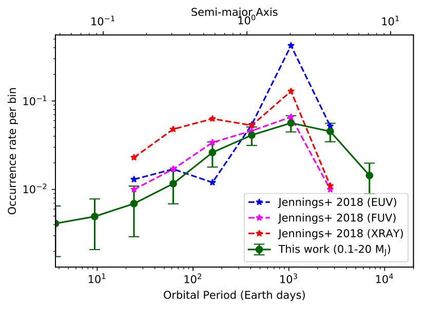 Figure 1
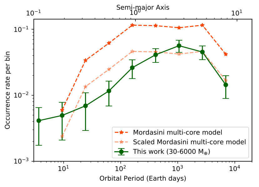 Figure 2
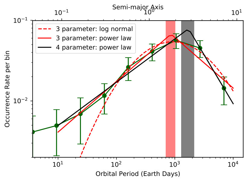 Figure 3
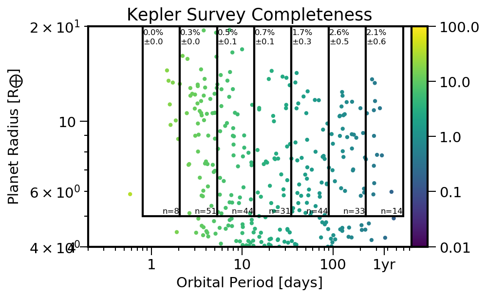 Figure 4
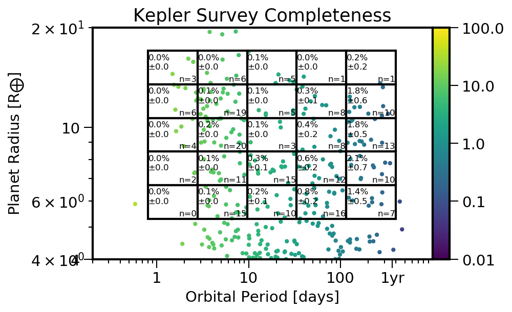 Figure 5
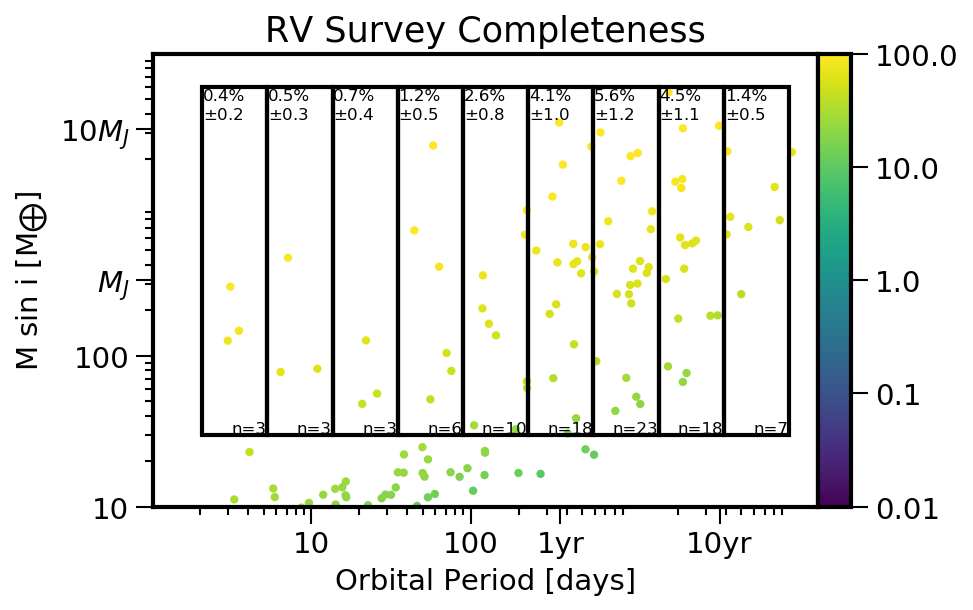 Figure 6
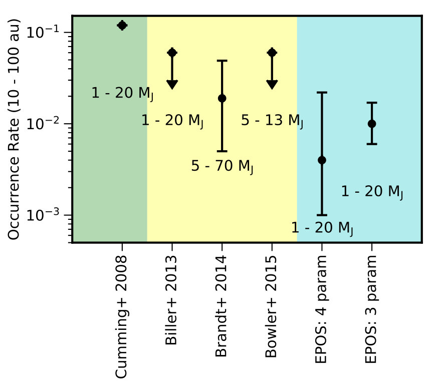 Figure 7
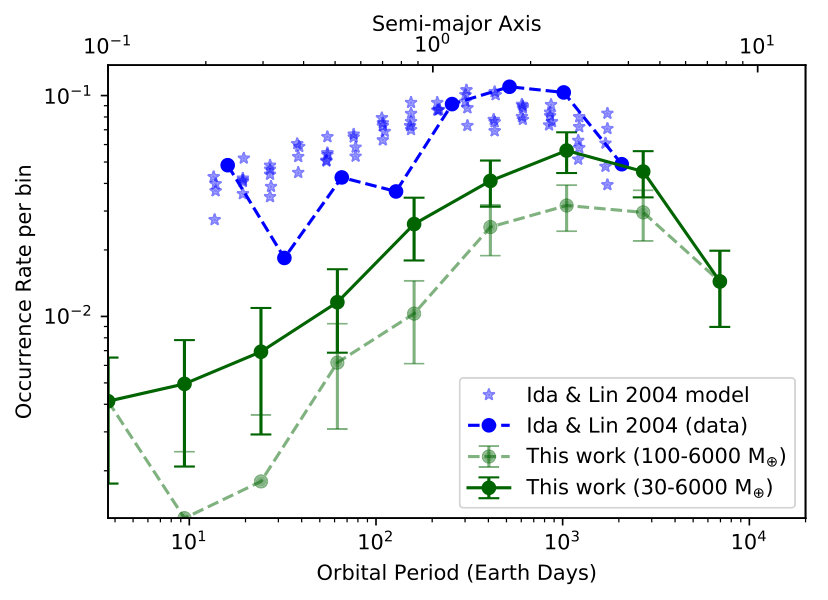 Figure 8
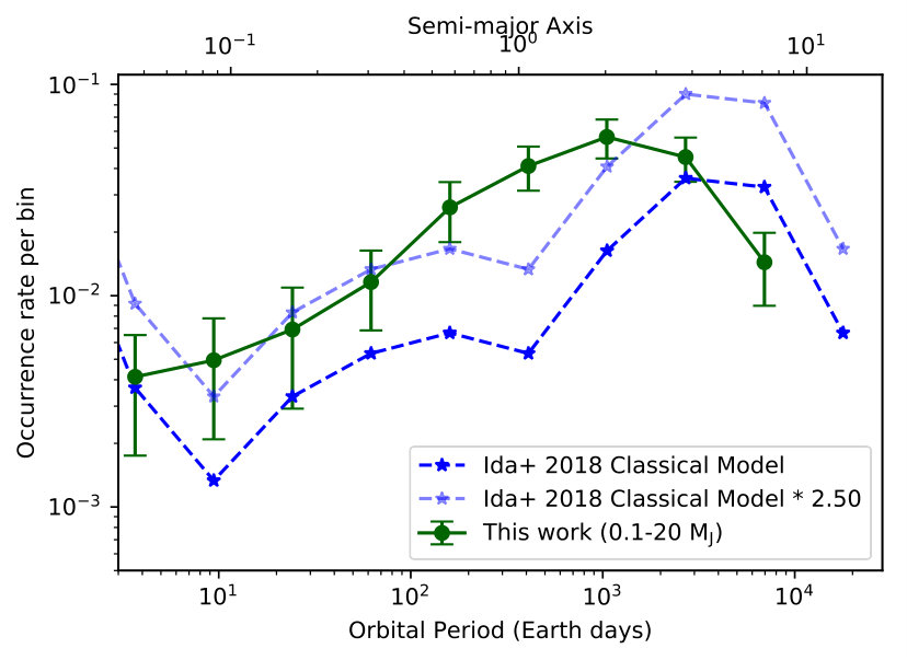 Figure 9
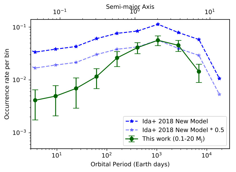 Figure 10
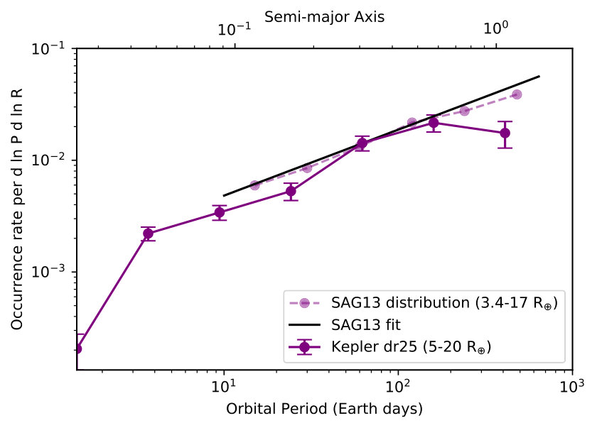 Figure 11
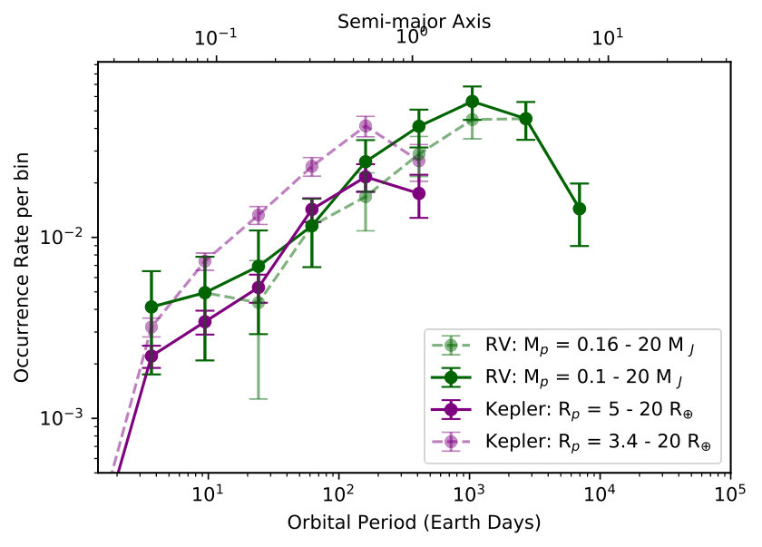 Figure 12
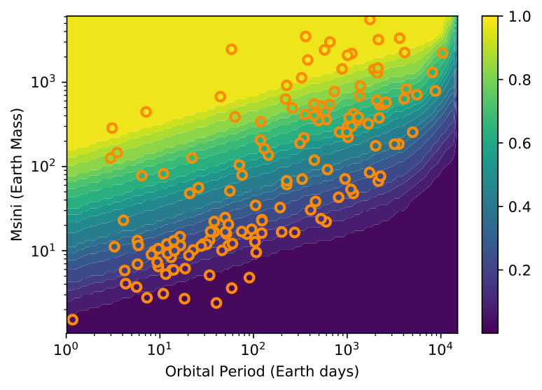 Figure 13
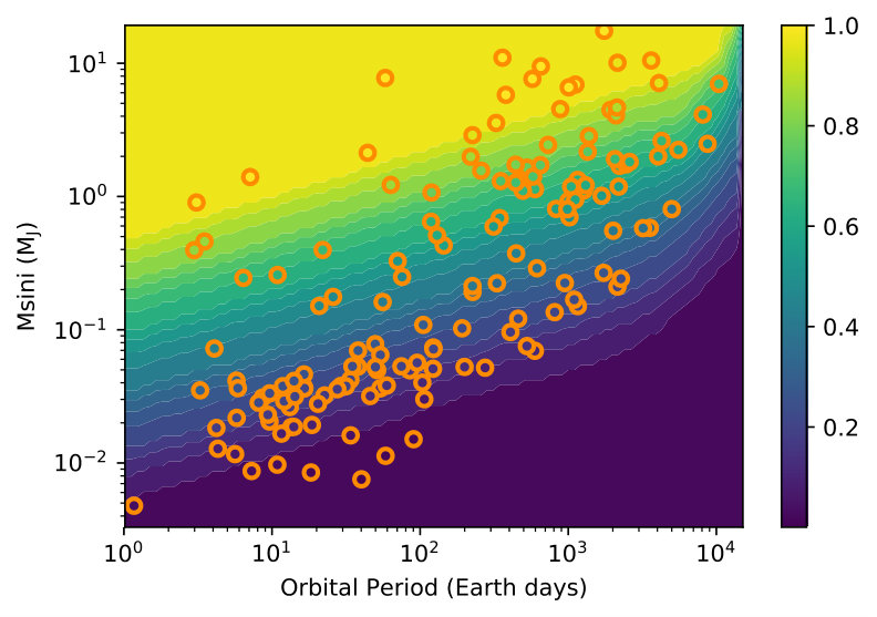 Figure 14
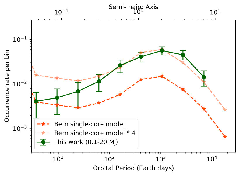 Figure 15
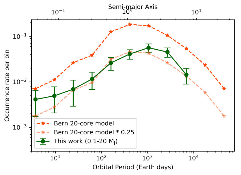 Figure 16
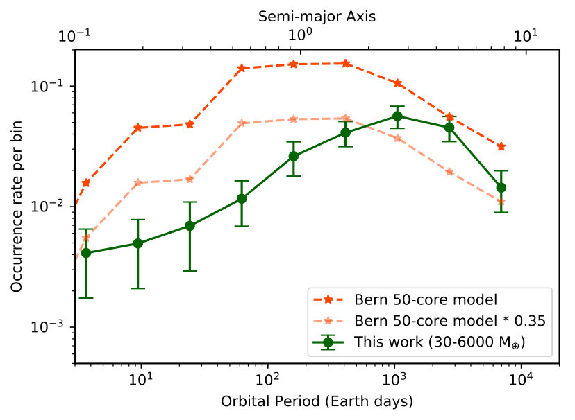 Figure 17
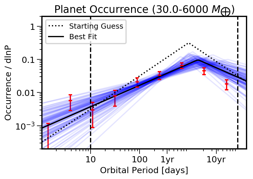 Figure 18
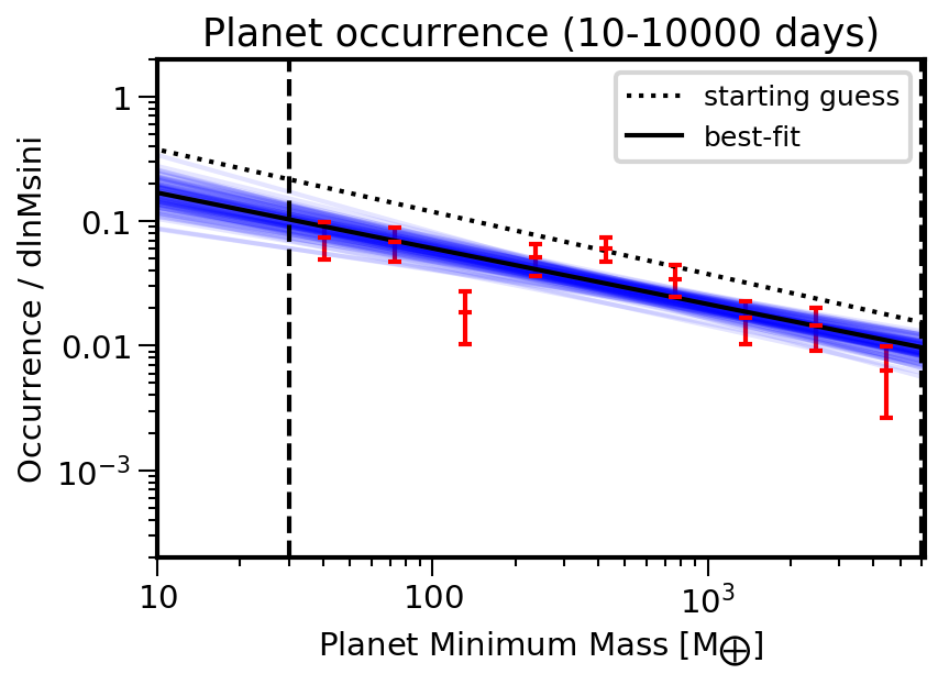 Figure 19
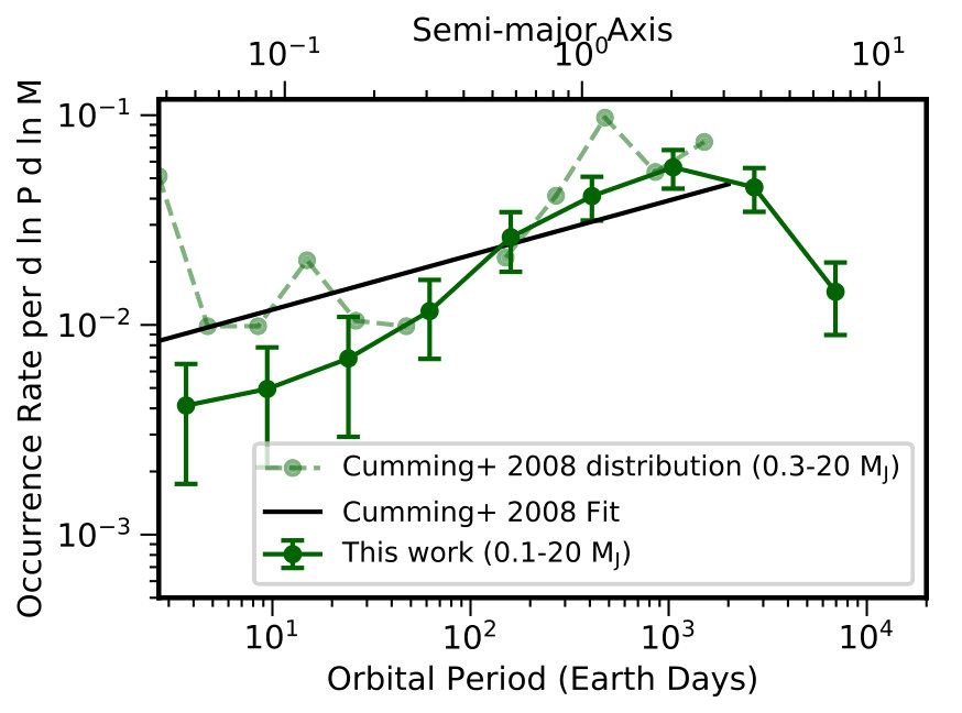 Figure 20
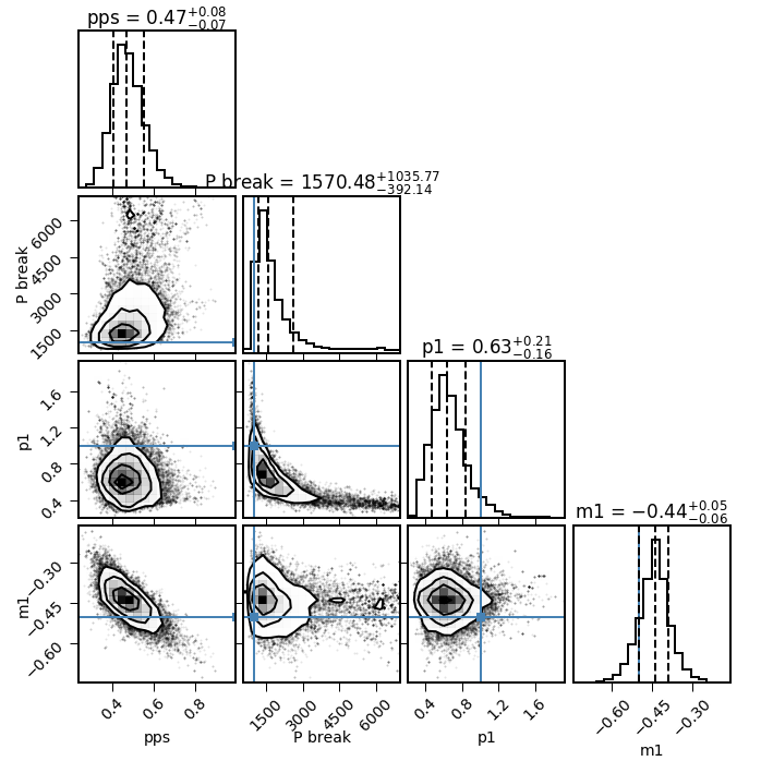 Figure 21
| Fit type | Function | Parameters | ||||
|---|---|---|---|---|---|---|
| Normalization | ||||||
| P | in days | P | Constant | |||
| scipy | Asymmetric | |||||
| Symmetric | ||||||
| Log-normal | ||||||
| epos | Asymmetric | |||||
| Symmetric | ||||||
| Fit type | Function | Free parameters | Direct Imaging Prediction (%) | |||
| (a) Giants | (b) Giants | (c) Jupiters | (d) Jupiters | |||
| au | au | au | au | |||
| scipy | asymmetric | 4 | 4.30 | 8.9 | 2.1 | 8.8 |
| symmetric | 3 | 5.94 | 7.9 | 2.9 | 7.8 | |
| single | 2 | 24.2 | 14.2 | 11.7 | 6.8 | |
| log-normal | 3 | 5.49 | 8.4 | 1.3 | 3.7 | |
| epos | asymmetric | 5 | ||||
| symmetric | 4 | |||||
| single | 3 | |||||
| Cumming+08 | single | 4 | 14 | - | 6.8 | 17-20 |
| Kopparapu+18 | single | 4 | - | 101 | - | - |
Peer Reviews
No public reviews on file for this paper yet. If you reviewed it on a platform where reviews are public (OpenReview, ICLR, NeurIPS, ICML), you can paste yours below so the community can read it here.
Videos
No videos yet. Explain this paper in a talk, walkthrough, or lecture? Add one.
Hints for a Turnover at the Snow Line in the Giant Planet Occurrence Rate
Lunar and Planetary Laboratory, The University of Arizona, Tucson, AZ 85721, USA
Earths in Other Solar Systems Team, NASA Nexus for Exoplanet System Science
Department of the Geophysical Sciences, The University of Chicago, Chicago, IL 60637, USA
Earths in Other Solar Systems Team, NASA Nexus for Exoplanet System Science
Lunar and Planetary Laboratory, The University of Arizona, Tucson, AZ 85721, USA
Earths in Other Solar Systems Team, NASA Nexus for Exoplanet System Science
Physikalisches Institut, Universität Bern, Gesellschaftsstrasse 6, CH-3012 Bern, Switzerland
Lunar and Planetary Laboratory, The University of Arizona, Tucson, AZ 85721, USA
Physikalisches Institut, Universität Bern, Gesellschaftsstrasse 6, CH-3012 Bern, Switzerland
Abstract
The orbital distribution of giant planets is crucial for understanding how terrestrial planets form and predicting yields of exoplanet surveys. Here, we derive giant planets occurrence rates as a function of orbital period by taking into account the detection efficiency of the Kepler and radial velocity (RV) surveys. The giant planet occurrence rates for Kepler and RV show the same rising trend with increasing distance from the star. We identify a break in the RV giant planet distribution between 2-3 au — close to the location of the snow line in the Solar System — after which the occurrence rate decreases with distance from the star. Extrapolating a broken power-law distribution to larger semi-major axes, we find good agreement with the planet occurrence rates from direct imaging surveys. Assuming a symmetric power law, we also estimate that the occurrence of giant planets between 0.1100 au is for planets with masses 0.1-20 and decreases to for planets more massive than Jupiter. This implies that only a fraction of the structures detected in disks around young stars can be attributed to giant planets. Various planet population synthesis models show good agreement with the observed distribution, and we show how a quantitative comparison between model and data can be used to constrain planet formation and migration mechanisms.
planetary systems — planets and satellites: formation — protoplanetary disks — methods: statistical — surveys
††software: NumPy (van der Walt et al., 2011), SciPy (Jones et al., 2001–), Matplotlib (Hunter, 2007), emcee (Foreman-Mackey et al., 2013), corner (Foreman-Mackey, 2016b), epos (Mulders, 2019), CRAN segmented (Muggeo, 2003, 2008)
1 Introduction
Giant planets, hereafter GPs, form while substantial gas is still present in disks, i.e. within 10 Myr (e.g., Pascucci et al. 2006). In the standard picture of planet formation (e.g., Raymond et al. 2005), terrestrial planets take much longer to form, of the order of hundreds of millions of years. As such, the presence, mass, and eccentricity of GPs directly impact the final location and mass of terrestrial planets (e.g., Levison & Agnor 2003). For example, Raymond (2006) finds that GPs inside roughly 2.5 au inhibit the growth of 0.3 M⊕ planets in the habitable zone of sun-like stars. In addition, GPs affect the delivery of water to terrestrial planets (e.g., Morbidelli et al. 2012), a key ingredient for the development of life as we know it.
The observed distribution of giant planets provides important clues to how and when they form. GPs preferentially form beyond the snow line since their formation is expected to be more efficient there due to an increased amount of solids as water vapor condenses onto ice (e.g., Kennedy & Kenyon 2008). In disks around young solar analogues, the snow line is expected to be between 2-5 au (e.g., Mulders et al. 2015a). For the Solar System, it is inferred to be at 2.5 au at the time of planetesimal formation from the gradient in composition of large main belt asteroids (e.g., DeMeo & Carry 2014). If indeed GPs preferentially form beyond the snowline, those detected within 1 au underwent significant migration, either through interaction with the gas disk (e.g., Goldreich & Tremaine 1980; Lin & Papaloizou 1986; Lin et al. 1996) or as a result of planet scattering (e.g., Rasio & Ford 1996; Weidenschilling & Marzari 1996; Ford & Rasio 2006; Chatterjee et al. 2008).
Alternatively, some theorists have argued that a substantial fraction of the hot and warm Jupiters could have formed in situ (e.g. see Batygin et al. 2016; Boley et al. 2016; Bailey & Batygin 2018).
Core-accretion planet formation models that include disk migration typically predict that the occurrence of giant planets increases with distance from the star within 1 au (e.g., Ida & Lin 2004a; Mordasini et al. 2009) but often show a break at larger distances. The exact shape of the distribution depends on the physics of planet formation: how planet cores grow and interact (e.g., Mordasini 2018), how quickly planets migrate through the disk (e.g., Ida & Lin 2008; Ida et al. 2018), and the timescale and mechanism by which the disk disperses (e.g., Alexander & Pascucci 2012). While superficial comparisons between these models and the detected GP population have been made (e.g., see Ida & Lin 2004b, a), a detailed statistical analysis in which survey completeness was taken into account has not been done.
The Kepler mission has provided detailed exoplanet population statistics for a large range of planet sizes close to their host stars (e.g., Howard et al. 2012). GPs show a rising occurrence rate out to the 1 au semi-major axis covered by Kepler (Dong & Zhu, 2013; Santerne et al., 2016). The radial velocity (hereafter RV) technique extends exoplanet detections well beyond au, but only for planets more massive than Neptune (e.g., Howard et al. 2010; Mayor et al. 2011; Wittenmyer et al. 2016).
The analysis of these RV data has established that GPs are much rarer than the Neptune and Super-Earths detected by Kepler with an occurrence of only 10% within a few years (see e.g., Table 1 in Winn & Fabrycky 2015). Early studies have also shown that the RV occurrence rate could be described by a power law in planet mass and orbital period for GPs 0.3-10 inside 2,000 days (e.g., Cumming et al., 2008). The frequency of these GPs was found to decrease with increasing mass and increase with period. However, direct imaging surveys recognized early on that such power law could not extend to the large orbital separations this technique is sensitive to, beyond 30 au, as they detected very few, if any, exoplanets (e.g., Kasper et al. 2007). Larger imaging surveys with improved instrumentation and analysis techniques are confirming that the frequency of GPs on wide orbits is indeed low, 1% (e.g., Bowler 2016; Galicher et al. 2016). Additionally, RV trend studies have been important to bridge the gap between the population of close-in planets detected via RV and the further way one discovered by direct imaging (Montet et al., 2014; Knutson et al., 2014; Bryan et al., 2016, 2018). Particularly relevant to our study is Bryan et al. (2016) who suggest a declining frequency of giants already beyond 3-10 au.
Here, we first compare the Kepler GP occurrence rate from the latest data release with the RV occurrence from Mayor et al. (2011) corrected for the survey completeness (Section 2.1). We show that beyond 10 days the occurrence of planets with masses 0.1-20 MJ (radii R⊕) match well, meaning that the RV GP occurrence rate can be used to extend that from Kepler. We find a break in the RV occurrence around – au (Section 2.3), close to the location of the snow line in our Solar System (e.g., Hayashi 1981; DeMeo & Carry 2014), and show that a broken power law better describes the observed GP frequency as a function of orbital period. In Section 2.4, we demonstrate that such broken power law also explains the low occurrence of directly imaged giant planets. We compare the overall occurrence rate distribution with that predicted by different planet formation models and find good agreement with a subset of these models (Section 3). Finally, we summarize our main results and discuss them in the context of the giant planets in our Solar System and the prominent structures detected in disks around young stars (Section 4).
2 Giant Planet Occurrence Rate
The intrinsic occurrence rate of planets can be calculated from the fraction of stars with detected planets in a survey and by making a correction for the number of non-detections. We calculate the average number of planets per star, hereafter occurrence rate, by averaging the inverse of the detection efficiency for each planet:
[TABLE]
where is the survey completeness evaluated at the location of each planet , the number of detected planets is and is the number of surveyed stars. The uncertainty on the occurrence rate is calculated from the square root of the number of detected planets per bin. Bin size is determined by dividing the period range (in log space) by the selected number of bins.
2.1 Radial Velocity Occurrence Rate
We calculate the RV GP occurrence rate using the detected planets and completeness reported in Mayor et al. (2011). The RV sample in Mayor et al. (2011) is a combination of the HARPS and CORALIE radial velocity surveys and includes a total of 822 stars and 155 planets.
We extract the survey completeness from Figure 6 in Mayor et al. (2011). This gives the probability that a planet with a given period P and minimum mass M sin i is detected and was calculated for each star and then averaged over all stars in the survey. Note that Mayor et al. (2011) adopt circular orbits to estimate the exoplanet detectability as most of their planets have eccentricities below 0.5 and Endl et al. (2002) have shown that eccentricities below this value do not substantially affect the RV detectability. Next, we recomputed the completeness over a finer grid by linearly interpolating on a uniform grid with Msini between 0.001-20 and period between 1-20,000 Earth days (see Figure 1).
In our analysis, we consider planets with a minimum mass in the range 0.1-20 , the lower value chosen to include all planets more massive than Neptune. We find that the GP occurrence rate increases with orbital period out to 1,000 days (see Figure 2 dark green curve) which is consistent with previous results, e.g., Mayor et al. (2011) and references therein. A more detailed analysis of the trend is described in Section 2.3. Note that the exact choice of upper and lower mass bins does not influence the broader trend described here (Figure 2 dark and light green curves). For the number of planets per Msini and orbital period bin, with corresponding completeness, see Appendix A. All data used in this paper and an example script to calculate planet occurrence rates are also available in the epos package (Mulders, 2019).
2.2 Comparison with Kepler Occurrence Rate
We calculate the GP occurrence rate from Kepler in a similar manner as RV. We use the planet candidate list and survey completeness from the latest DR25 Kepler data release (Mathur et al., 2017; Thompson et al., 2018) as described in Mulders et al. (2018). Exoplanet eccentricities are not implemented in our study (or in the epos simulations), effectively assuming circular orbits. For the completeness, planets with small eccentricities (e0.3) have also been assumed to be on circular orbits as any difference in the transit probability and duration is negligible, see Mulders et al. (2015b). The completeness and number of planets per radius and orbital period bin is reported in Appendix A.
Since Kepler measures planet radii and not masses, we use a mass-radius relation to select a planet radius bin that covers a similar RV planet mass bin. With the mass-radius relation in Chen & Kipping (2016), we set the lower value for the radius bin to 5 , as it is within 1 of the best-fit relation for 30 , while the upper value is set to 20 . Using a sample of planets with known masses and radii, Lozovsky et al. (2018) have recently shown that planets with radii 4 must have a significant H-He atmosphere (more than 10% of the planetary mass). Hence, our choice of 5 as the lower radius ensures that we include gaseous planets in our analysis. Note however that the trend of increasing occurrence with orbital period does not depend too much on the exact choice of radius bins (Figure 2, light and dark purple curves).
As can be seen in Figure 2, the Kepler and RV occurrence rates versus orbital period are very similar. While Kepler and RV potentially probe different stellar populations as well as different planet size/mass regimes as described above, the rates are the same within 1 for the bulk of the population which is beyond 10 days. In the Hot Jupiter regime, i.e. inside 10 days, we find that the Kepler occurrence rate is lower (0.510.08%) than the RV occurrence (0.90.5%), as reported in previous studies (e.g., Figure 9 in Santerne et al. 2016), though these values are consistent within 1 (see also Petigura et al. 2018).
2.3 Turnover at 2.5 au
As discussed in the previous subsections the occurrence rate of GPs increases with orbital period for periods where the RV and Kepler surveys overlap. However, beyond 1,000 days the RV curve appears to have a turnover111Note that a turnover is also seen in the cumulative rate of giant planets (Msin*i*M⊕) presented in Mayor et al. (2011), their Figure 8.. We perform three statistical tests to characterize the break in the distribution.
First, we use the CRAN package segmented to evaluate the statistical significance of a breakpoint. segmented determines if an observed distribution can be best described by one or multiple linear segments. It does not use a grid search but rather an iterative procedure, starting only from possible breakpoints, and taking advantage of the fact that the problem can be linearized (Muggeo, 2003, 2008). It also uses a bootstrap restarting (Wood, 2001) to make the algorithm less sensitive to the starting values. Since RV occurrence rates are typically better described by power-laws than linear functions (e.g., Cumming et al. 2008), we fit the log of the RV occurrence rate per bin vs the log of the period. For planet masses 0.1-20 and periods days, segmented finds a break at 1,766 days ( au) and a probability that the distribution can be described by a single power-law (or line in log space) as low as 0.17% using the associated davies test222The same tests applied to the 0.16-20 range used in Mayor et al. (2011) find a break at 3 au with a somewhat larger probability of 1.8% that a single power-law can describe the RV occurrence between 1 and 10,000 days..
Motivated by these results, we then fit the occurrence rate and associated uncertainty with a broken power law in orbital period utilizing the optimize function from the SciPy package in Python:
[TABLE]
where N is the number of planets per period bin, P is the orbital period, A is a normalization factor, is the location of the break in the period distribution and, and are the power-law indices before and after the break, respectively.
For an asymmetric broken power-law (4 parameters fit), is found to be between 12852149 days (2.33.2 au) with =0.530.09 and =-1.220.47333The results for a larger minimum mass of 0.16 MJ are very similar: =16022086 days while =0.480.09 and =-1.210.47 beyond.. This best fit gives a low reduced of 0.12 suggesting that we might be over-fitting the data. Hence, we also consider a 3-parameter fit with a symmetric broken power-law in order to better constrain the slope after the break. In this case, is found to be closer in, between 6981020 days (1.52.0 au), and ==0.630.11, basically set by the larger number of data points inside . This also gives us a low reduced of 0.11.
A log-normal distribution, as that used for GPs around M dwarfs (Meyer et al., 2018), returns a between 8141024 days. Given the symmetry of this function around the break point it is not surprising this is consistent with that obtained from the symmetric broken power-law fit. In this case the reduced is 0.74, higher than in the case of the power-law functions.
Additionally, we use the Bayesian Information Criterion (BIC) test to determine which fit is statistically better. BIC is a criterion for model selection among a finite set of models in which the model with the lowest BIC is preferred. It is based, in part, on the likelihood function and is defined as BIC = nln(sse/n) + kln(n) where n is the number of observations, k is the number of variables and sse is the squared sum of the residuals. The bigger the difference in the BIC scores of two models (usually 2), the worse the model with the higher BIC score is. We find that the asymmetric (BIC score: -29.54) as well as the symmetric broken power law fit (BIC score: -31.62) were indeed better fits than the single power law fit (BIC score: 12.16) since they have significantly lower BIC scores. Figure 3 provides a visual comparison of these best fit relations while Table 1 summarizes the best fit parameters.
Finally, we also use epos444https://github.com/GijsMulders/epos version v1.1 (Mulders, 2019), which uses the forward modeling approach described in Mulders et al. (2018), to constrain the occurrence rate of GPs. epos simulates exoplanet survey yields from an intrinsic distribution of planet properties by taking into account detection biases such as viewing inclination, and constrains this distribution by adopting a Markov Chain Monte Carlo approach with the emcee Python algorithm (Foreman-Mackey et al., 2013).
For this analysis, we adjust epos for use with radial velocity surveys by constraining the distribution function of planet mass and orbital period directly from the observed survey data, without random draws. We opt not to use the Monte Carlo simulation in epos because the number of detected planets in the RV survey is significantly lower than detected in the Kepler, increasing the associated noise. Instead, we replace the steps where we generate a synthetic planet population by random draws and remove non-detectable planets to obtain a detected planet sample, by the following steps.
First, we adjust the planet distribution function from Equation 2, to include a planet mass dependence.
[TABLE]
where is a normalization factor, is the broken-power law period distribution described in Equation 2 (without the normalization factor ), and is the power-law index of the planet mass distribution . The normalization factor is set such that the integral of the function over the simulated planet period and mass range equals the average number of planets per star.
Then, we convolve the true mass distribution with a function to take into account random viewing angles
[TABLE]
where is the true planet mass see Appendix B for derivation, to obtain the simulated distribution with is function of .
Last, we multiply this distribution with the detection efficiency, , to obtain a detectable planet distribution function:
[TABLE]
We then compare this distribution function to the observed planet distribution, , using a one-sample KS test to replace the two-sample KS test in epos.555We have verified with epos that using minimum mass instead of true mass leads to only a small underestimate in planet occurrence rates for such wide mass bins, only 12.9% of the occurrence itself. We did this by fitting the Msini distribution instead of the true mass distribution with epos and calculating the percentage change in the normalization factors. We then proceed as in Mulders et al. (2018) to identify the best parametric fit for the RV exoplanet population using emcee. A triangle plot of the best fit parameters for the symmetric power-law fit can be seen in Appendix B. This procedure has been implemented in version 1.1 of epos.
When modeling the period distribution with an asymmetric power-law, epos finds a break at days with = and after the break, in agreement withing 1 of our asymmetric power-law fit using scipy. The posterior distribution of planet orbital period and mass are shown in Figure 4, for the symmetric epos fit. The corner plot showing the projections of the likelihood function can be found in Appendix B. In the case of a symmetric power-law distribution, epos finds a break at days with a slope of which is within 1 of the values found with SciPy for a symmetric power-law in period. The best fit power law index for the mass distribution is for both the symmetric and asymmetric power-law in period.666We increased the lower mass limit to 0.3 MJ and 0.5 MJ and found that there was no sigificant change in and with their respective at 13463470 days and 15043190 days which is consistent within 1 of the 0.1 MJ value. Using the BIC test in epos, we found that the asymmetric (BIC score: 23.5) as well as the symmetric broken power law fit (BIC score: 18.9) were indeed better fits than the single power law fit (BIC score: 34.2) since it has a lower BIC score. Here, again, the broken power-law is preferred over the single power-law since the difference in BIC scores is 10. A summary of our best fit values can be found in Table 1.
Hence, we conclude that there is evidence for a break in the RV GP occurrence rate, although the slope beyond the break is not well constrained because the RV data only extend to 104 days. An RV data set with a longer baseline is needed to put stronger constraints on the slope after the break. While we prefer a 3-parameter solution given the lack of observational constraints, where the slope is constrained mostly from the distribution before the break, as also motivated by Meyer et al. (2018), the fitted slope of the 4-parameter solution has a large uncertainty that is consistent with the 3-parameter solution to within 1 . The break has important implications when extrapolating GP occurrence rate at semi-major axis relevant for direct imaging surveys (Section 2.4). Additionally, it is important for our theoretical understanding of how and where giant planets form (see Section 3).
2.4 Predictions for Direct Imaging
Direct imaging surveys are mostly sensitive to planets at large (10 au) separations. Such surveys have found that GPs more massive than 5 are rare, with an occurrence of only 1%, at separations between a few tens to a few hundreds au (e.g., Bowler 2016; Galicher et al. 2016). This value is lower than the RV GP occurrence rate inside a few au, see e.g. Figure 1. Integrating within a period of 2,000 days Cumming et al. (2008) reported an occurrence of 10% for 0.3-10 MJ, an order of magnitude higher than the rate of directly imaged planets. Hence, it was realized early on that the single RV power law in semi-major axis cannot extend at large separations (e.g., Kasper et al. 2007; Chauvin et al. 2010; Nielsen & Close 2010). Recently, Bryan et al. (2016) conducted an RV+imaging survey of stars with already known exoplanets and found that the frequency of GP companions declines with semi-major axis beyond 3-10 au. Here, we show that the turnover we find in the RV occurrence rate at 2.5 au naturally explains the high occurrence of GPs within a few au and the low occurrence rate of planets further out.
Our analysis of the Mayor et al. (2011) RV planets, including their survey completeness, recovers previous results obtained with a single power law (see Appendix C) and, most importantly, suggests that the GP occurrence does not increase with orbital period beyond 3 au (see Section 2.3). Using functions that take into account this turnover, we calculate yields at large semi-major axis and find that they are significantly lower than those predicted by a single power law, see Table 2.
For instance, when we extrapolate the scipy asymmetric and symmetric power laws at the location where direct imaging is most sensitive to, i.e. 10-100 au, and assuming a flat planet mass dependence between 0.1-13 , we predict a GP occurrence rate of 4.3% and 5.9% respectively (column (a) in Table 2). epos finds similar values, albeit the uncertainties on the occurrence rate are large for the 4-parameter fit due to the uncertainty in the slope after the break.
In the same period range, the occurrence of Jupiters, planets with masses between 1 and 13 , is even lower (column (c) in Table 2), well in agreement with that from direct imaging surveys. On the other hand, for GPs across all the mass and period ranges in Table 2, the occurrence rates estimated using a single power law in period are an order of magnitude to several orders of magnitudes higher than those obtained with broken power laws as well as a log-normal fit.
A visual summary of GP occurrence rates in the semi-major axis range directly relevant to direct imaging (10100 au) is shown in Figure 5. The figure includes the extrapolated rate using the single power law in period reported in Cumming et al. (2008), three representative occurrence rates from direct imaging surveys (Biller et al., 2013; Brandt et al., 2014; Bowler et al., 2015), as well as the epos values reported in Table 2. As can be seen in the figure, the epos rates obtained with a broken power law in period are within 1 of the direct imaging values from Brandt et al. (2014) and consistent with the upper limits reported in Biller et al. (2013) and Bowler et al. (2015). The extrapolated rate from Cumming et al. (2008) using a single power-law is too high, clearly inconsistent with the low occurrence of GP reported by direct imaging surveys. Hence, we can conclude that the broken power-law fit is more consistent with the observed GP occurrence rates at larger orbital periods.
Recently, Kopparapu et al. (2018) extrapolated the Kepler SAG13 occurrence rates between au to evaluate the GP yield of future direct imaging missions. As the extrapolation is based on the assumption that a single power law in period describes well the GP occurrence (see also Appendix C), the yield is very large, basically each star has a GP between 2-20 au (see column (b) in Table 2). However, if a broken power-law (or log-normal) distribution better describes the GP occurrence rate, Table 2 shows that the occurrence of planets is about a factor of 5 lower than that reported in Kopparapu et al. (2018). This has important implications for the science goals that can be achieved by future direct imaging missions.
3 Comparison with theoretical models
As shown in Section 2, the occurrence rate of GPs rises with orbital period, peaks between 2-3 au, and decreases beyond. Such a feature could be an imprint of giant planet formation and/or subsequent evolution in the disk. Within the core accretion paradigm, giant planet formation happens as a two-step process: first a solid core with a critical mass of order 10 M⊕ must form, then the rapid accretion of a massive gaseous envelope sets in. As GPs form in a gaseous disk, they must subject to gas-driven migration through tidal interaction with their nascent disk. As in most models they form beyond the snow line, inward migration likely plays a role in shaping the semi-major axis distribution of GPs at short orbital periods. However, it is also possible that the GPs could form in situ (e.g., see Batygin et al. 2016) or, under favorable conditions, they could migrate outward (e.g., see D’Angelo & Marzari 2012).
As the time scale for inward type-II migration is typically shorter than the disk lifetime, GPs will be accreted onto the star if migration is not stopped. There are several mechanisms proposed to halt the inward migration and create the observed population of warm giants: interaction with other GPs; photoevaporation carving a hole in the disk; or slow type-II migration that have been included in population synthesis models.
In this section, we make a qualitative comparison between planet occurrence rates and planet population synthesis models that employ these different physical mechanisms. We use the grid of surviving planets from Jennings et al. (2018) and Ida et al. (2018), and two grids from the DACE database based on the simulations in Mordasini (2018). For each model, we calculate the predicted occurrence rate as the fraction of simulated star systems that form a planet with mass larger than 0.1 in each period bin in order to directly compare to the curves we computed in Section 2.
3.1 Formation via core accretion: Ida et al. 2018
Ida & Lin (2004b, a) were the first to carry out core accretion population synthesis models. They used the results of N-body simulations to model the accretion phase of cores starting from planetesimals and Kelvin-Helmholtz contraction for the accretion of gas onto cores. While Type I migration is not included, protoplanets large enough to open a gap are subject to Type II migration, and move inward.
Recently, Ida et al. (2018) published updated synthetic planet populations for two different implementations of Type II migration, classical and new. The classical model assumes that Type II migration is associated with gas accretion through the disk, as in Ida & Lin (2004b, a). The new model is based on recent high-resolution simulations by Kanagawa et al. (2018) showing that there is a disconnect between the migration of the gap-opening planet and the disk gas accretion, resulting in a reduced migration rate. The slower Type-II migration results in a larger fraction of planets being retained at short orbital periods.
As can be seen in the top panel of Figure 6, the classical model indeed underpredicts the number GPs between 10-1000 days by a factor 2.5. However, the slope of the predicted orbital-period distribution in this region is similar to the estimated planet occurrence rates (dark green curve). There is no clear indication of a turnover within the observed range ( days). On comparing the scaled model to the data, we get a high value of 186.65, thus implying that this model is not a good fit to the data.
The orbital period distribution of the new model (see Figure 6, bottom panel) is much flatter than observed. The new model overproduces the number of giant planets at all orbital periods, in particular those at the shortest orbital periods. We scaled down the model to better fit the peak of the RV distribution. The slope of the orbital period distribution is much flatter than the observed one. The new model does shows a turnover at a period of days that matches well with the observed break in the planet occurrence rate distribution. Here, we get a value of 91.84 hinting that this new model is a better fit than the classical one.
As the observed RV distribution lies in between the new and classical model, a direct comparison between model and observations may be used to calibrate the strength of Type II migration.
3.2 Formation via core accretion and multi cores interaction: The Bern Model
As in Ida & Lin (2004b), the GP formation model used in Mordasini (2018) relies on the core accretion paradigm. However, these more recent population synthesis include updated prescriptions for the evolution of the protoplanetary disk as well as for migration, including Type I migration of cores that are not massive enough to open gaps (Dittkrist et al., 2014) and directly calculate the N-body interaction of concurrently forming protoplanets (Alibert et al., 2013).
In this contribution, we compare two populations obtained from an updated version of the Mordasini (2018) model. Each population comes from a different type of model: one model includes just one planetary embryo that can grow into a GP (single-planet) while the other includes multiple embryos that can form multiple GPs (multi-planet). The multi-planet model additionally uses a N-body module to study concurrent growth and interactions of multiple planetary embryos that are injected into each disk. The results from these simulations will be presented in more details in Emsenhuber et al. (in prep.).
The single-planet simulations predict an increase in the GP occurrence rate between 1001000 days (top panel in Figure 7), as observed (dark green curve in the same figure). However, they under-predict the overall number of GPs at those orbital periods by a factor of 4 when compared to the RV occurrence rate. When scaled to match the observed RV peak, the single-planet models over-predict the number of GPs inside 30 days but the turnover beyond 1,000 days is very similar to the observed one giving us a value of 39.12.
The GP occurrence rate for the multi-planet simulations with initially 20 embryos per disk lower panel of Figure 7) has a similar shape as the observed one, i.e. increasing occurrence with semi-major axis and a turnover after which occurrence rate decreases. In order to match the occurrence rate, results need to be scaled down by a factor of 0.25, implying that only 1 in 4 stars would form the simulated systems. On comparing the scaled model to the RV data, we get a low value of 6.96, suggesting that the scaled model is a good fit to the data.
The two models have overall the same shape, except for the inner planets. The difference in the total occurrence rate follows from the increase of the number of embryos in the multi-planet model, which increases the chance of forming GPs. The overall similar shape of the single- and multi-core models tell us that the planet-planet interactions do not significantly affect the GP formation process. We expect however that a further increase of the number of embryos could affect these results.
The single-planet model overproduces inner planets whereas the multi-planet underproduces them. In the single-planet model, inward migration of GPs is very efficient, which causes the pile-up of HJs. For the multi-planet model, migration is less efficient, possibly due planet-planet interactions which helps stabilizing GPs which are in mean motion resonances.
3.3 GP trapping due to photoevaporation disk clearing: Jennings et al. 2018
The models by Jennings et al. (2018) explore the late evolution of fully formed GPs in viscously evolving and photoevaporating disks, similarly to Alexander & Pascucci (2012) and Ercolano & Rosotti (2015). Unlike Ida & Lin (2004a, b) and Mordasini (2018), they do not simulate the formation of planetary cores nor the subsequent atmospheric accretion. However, they do have a more detailed treatment of the disk clearing phase.
The simulation of Jennings et al. (2018) begins with a viscously evolving disk irradiated by either a pure EUV, X-ray, or FUV-dominated stellar flux. A planet ranging in mass from 0.5 to 5 is inserted at 5 au at a random time between 0.25 Myr and the time of disk clearing. The planet moves inward through Type II migration, further accretes mass as gas flows across its gap, while the disk viscously evolves and is being photoevaporated. After a few Myrs, the mass accretion rate falls below the wind photoevaporative rate, hence a gap opens in the disk which can slow down or completely stop the migration of giant planets. The location of the gap, and hence the final location of planets, depends on the stellar high energy photons driving photoevaporation, i.e. 0.8 au for EUV, 1.7 au for X-ray and 4 au for FUV.
Jennings et al. (2018) end their simulations either when the disk surface density is or when the migrating planet reaches a separation 0.15 au from the star. A thousand of these simulations are conducted for each of the three photoevaporative profiles, by varying only the photoevaporative mass loss rate, planet formation time, and initial planet mass.
On comparison with the RV occurrence rates (Figure 8), we find that the FUV model (magenta curve) has an occurrence rate that best matches the observed rates and slope between 30-1000 days with a value of 29.12. The X-ray model (red curve) does a fairly good job for the GP occurrence at 1,000 days but tends to over-predict the number of GPs at shorter orbital periods ( value of 288.56). Finally, the EUV model over predicts the increase in planet occurrence around 1,000 days or shows an increase in planet occurrence between 100-1000 days that is steeper than observed, after scaling to the peak. Since EUV creates a gap closer in than the FUV or X-ray case, the viscous timescale to drain the inner disk is shorter, i.e. a surviving planet will be more likely stalled at the gap opening location which creates a larger pile-up than observed. The EUV model gives an extremely high value of 1947.84 meaning that it is not a good match to the data. All models show a break at 1,000 days but a steeper drop than the data beyond. However, the steep drop likely results from no planets being injected outward of 5 au.
4 Summary & Discussion
We computed the giant planet occurrence rates out to days based on the planet detections and simulated survey completeness from the HARPS and CORALIE radial velocity surveys (Mayor et al., 2011). We characterize the shape of the orbital period distribution and evaluate our findings in the context of directly imaged planets and planet formation models. We find that:
The occurrence of giant planets from Kepler (radii R⊕) and RV (masses 0.1-20 MJ) show the same rising trend with orbital period for periods between – days. As pointed out in the past (e.g., Santerne et al. 2016), the Kepler occurrence of hot Jupiters (10 days) is about half of the RV one but we show that the value is within 1 of the large uncertainty associated with the RV data. 2. 2.
There is evidence for a break in the GP occurrence rate around 1,000-2,000 days. For solar-mass stars these periods correspond to semi-major axis – au, bracketing the location of the snow line in the Solar System. 3. 3.
The break in GP occurrence rate decreases the giant planet yields when extrapolated to orbital periods accessible by direct imaging surveys. Using epos we calculate an occurrence of for planets more massive than Jupiter between 10-100 au, in agreement with the values reported from direct imaging surveys. 4. 4.
Different planet population synthesis based on core accretion and including Type-II migration produce a turnover in the GP occurrence rate around the snow line. We find that models with multiple planet cores per disk qualitatively seem to be a better match to the observed distribution.
In a recent study Wittenmyer et al. (2016) used their Anglo-Australian Planet Search survey to estimate that only of solar-type stars have a Jupiter analog, i.e. a giant planet with masses between 0.3-13 MJ located between 3 and 7 au. In the same planet mass and semi-major axis range, we derive an occurrence of from the epos best fit symmetric power law, in agreement with Wittenmyer et al. (2016) within the quoted uncertainties. Thus, it appears that Jupiter analogs are rather rare.
Using the same best fit model, we also calculate an integrated frequency for planets between 0.1100 au of for 0.1-20 and for planets more massive than Jupiter (1-20 ). These statistics are interesting in the context of structures recently identified in protoplanetary disks. For example, van der Marel et al. (2016) analyzed an unbiased sample of disk candidates based on Spitzer catalogs and retrieved a frequency of dust cavities larger than 1 au in radius of 23% . While about half of them can be explained as the result of late disk evolution and dispersal by star-driven photoevaporation (Ercolano & Pascucci, 2017), the other half are more likely to host one or more GPs. As this statistic is lower than our integrated occurrence of 0.1-20 , there appears to be enough mature GPs to explain the frequency of transition disks. Rings and narrow gaps are very common in disk surveys biased toward the brightest millimeter sources, with an occurrence as high as 85% from the ALMA DSHARP survey (Andrews et al., 2018; Huang et al., 2018). However, this number goes down to 38% in the Taurus disk survey from Long et al. (2018) which covers fainter millimeter disks, hence it is more representative of the entire disk population. Considering that the fraction of disks in Taurus is 75% (Luhman et al., 2009), the fraction of structures from this survey is then 28%. This value is similar to our occurrence of 0.1-20 planets between 0.1-100 au. Hence, there is no disagreement between the count of mature exoplanets and disk structures if only one GP is necessary to reproduce all the observed structures in each disk and migration re-distribute the forming GPs over a large range of semi-major axis, from 0.1 out to 100 au. However, if multiple structures cannot be explained by one GP alone, it would be important to explore if planets less massive than 0.1 could open such gaps as their occurrence is larger than that of GPs both inside as well as outside the snow line (Suzuki et al., 2016; Pascucci et al., 2018).
Going forward, these occurrence rate distributions can be used to update planet yield estimates for future missions and provide context for Gaia, which is expected to detect over 20,000 high-mass ( MJ) planets out to 5 au (e.g., Perryman et al. 2014). The large sample size from Gaia may reveal structures around and beyond the snowline and place more stringent constraints on planet migration and formation models.
R.B.F. would like to thank Kyle A. Pearson for his valuable insight and expertise while recalculating the Mayor et al. (2011) completeness. We would also like to thank Shigeru Ida and Jeff Jennings for sharing simulated planet populations. This paper includes data collected by the Kepler mission. Funding for the Kepler mission is provided by the NASA Science Mission directorate. This material is based upon work supported by the National Aeronautics and Space Administration under Agreement No. NNX15AD94G for the program Earths in Other Solar Systems. The results reported herein benefited from collaborations and/or information exchange within NASA’s Nexus for Exoplanet System Science (NExSS) research coordination network sponsored by NASA’s Science Mission Directorate.
Appendix A Occurrence Rates
Figure 9 shows the Kepler and RV survey completeness and the number of planets per radius/Msini and orbital period bin.
Appendix B epos parametric fit
Figure 10 shows the best fit parameters and associated uncertainties with a run for a symmetric power-law fit in period and a single power-law in Msini that used 50 walkers for 1000 Monte Carlo iterations and a 200-step burn-in.
The conversion from planet mass distribution to distribution goes as follows. For a planet of mass the measured minimum mass is . For random viewing angles, the inclination is distributed across as
[TABLE]
The distribution of minimum mass is then:
[TABLE]
and substituting gives
[TABLE]
for and if .
Appendix C Over-prediction at large orbital periods when using a single power-law
The NASA’s Exoplanet Science Analysis Group-13 (SAG-13) collected occurrence rates from different teams. The occurrence of GP (3.4 - 17 ) is fitted with a single power law within 10 - 640 Earth days. Similarly, Cumming et al. (2008) have used a single power-law in order to explain the GP population of the RV data for GPs (0.3 - 20 ) out to 2,000 days. These single power-laws have been extrapolated in recent literature to predict the occurrence of GPs at large orbital distances. An example of these fits can be seen in Figure 11. The left panel shows the fit to SAG-13 distribution (3.4 - 17 ). In order to evaluate the planet yield of direct imaging missions, Kopparapu et al. (2018) further extrapolate this fit between 1.620 au to get a GP occurrence of 101%.
Cumming et al. (2008) extrapolate the single power-law distribution to estimate the number of planets within 20 au to be 1719%. They find the slope of the period distribution to be 0.26 0.1 as compared to a slope of 0.53 0.09 (before the break) that we find when we fit a broken power law to the RV distribution. We were also able to reproduce the Cumming et al. (2008) value for the slope when we fit a single power-law to the RV curve. Upon extrapolation of the Cumming et al. (2008) power-law between 10 - 100 au, we get an occurrence rate of 25%.
Both the Cumming et al. (2008) and the SAG-13 extrapolated values are much higher that those from direct imaging observations (see Figure 5) as well as those calculated using a broken power-law in this paper (see Table 2).
The reference list from the paper itself. Each links out to its DOI / PubMed record.
- 1Alexander & Pascucci (2012) Alexander, R., & Pascucci, I. 2012, Monthly Notices of the Royal Astronomical Society: Letters, 422, L 82
- 2Alibert et al. (2013) Alibert, Y., Carron, F., Fortier, A., et al. 2013, Astronomy & Astrophysics, 558, A 109
- 3Andrews et al. (2018) Andrews, S. M., Huang, J., Pérez, L. M., et al. 2018, ar Xiv preprint ar Xiv:1812.04040
- 4Bailey & Batygin (2018) Bailey, E., & Batygin, K. 2018, The Astrophysical Journal Letters, 866, L 2
- 5Batygin et al. (2016) Batygin, K., Bodenheimer, P. H., & Laughlin, G. P. 2016, The Astrophysical Journal, 829, 114
- 6Biller et al. (2013) Biller, B. A., Liu, M. C., Wahhaj, Z., et al. 2013, The Astrophysical Journal, 777, 160
- 7Boley et al. (2016) Boley, A. C., Contreras, A. G., & Gladman, B. 2016, The Astrophysical Journal Letters, 817, L 17
- 8Bowler (2016) Bowler, B. P. 2016, Publications of the Astronomical Society of the Pacific, 128, 102001