Transmission in Graphene through Time-oscillating Linear Barrier
El Bou\^azzaoui Choubabi, Ahmed Jellal, Miloud Mekkaoui

TL;DR
This paper investigates how Dirac fermions in graphene transmit through a time-oscillating linear barrier, deriving transmission probabilities for multiple modes by solving the Dirac equation and constructing a transfer matrix.
Contribution
It introduces a method to analyze transmission in graphene with a time-dependent barrier by solving the Dirac equation and calculating transmission for multiple oscillation modes.
Findings
Transmission probabilities depend on oscillation modes
Numerical approach limited to low quantum channels
Provides a framework for analyzing time-dependent barriers in graphene
Abstract
Transmission probabilities of Dirac fermions in graphene under linear barrier potential oscillating in time are investigated. Solving Dirac equation we end up with the solutions of the energy spectrum depending on several modes coming from the oscillations. These will be used to obtain a transfer matrix that allows to determine transmission amplitudes of all modes. Due to numerical difficulties in truncating the resulting coupled channel equations, we limit ourselves to low quantum channels, i.e. , and study the three corresponding transmission probabilities.
Click any figure to enlarge with its caption.
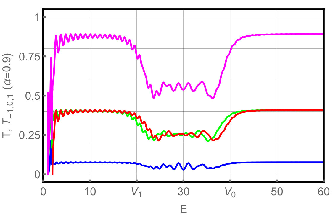 Figure 1
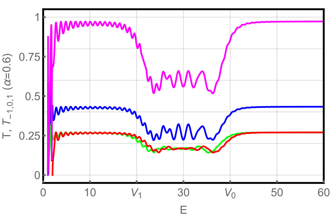 Figure 2
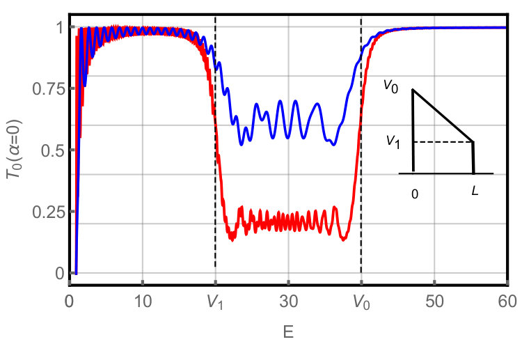 Figure 3
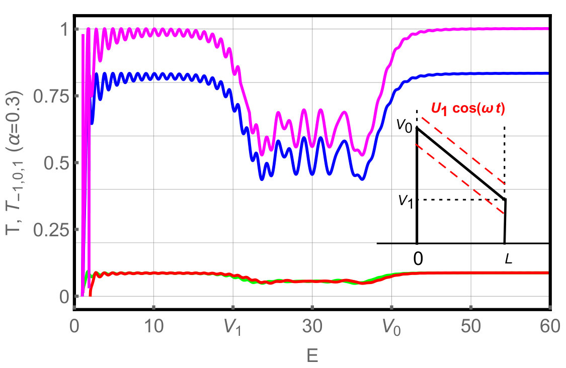 Figure 4
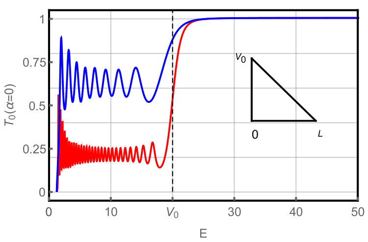 Figure 5
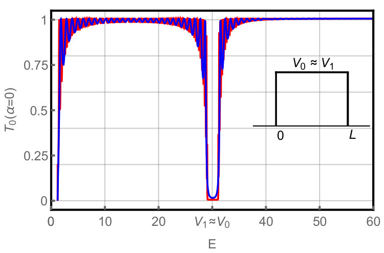 Figure 6
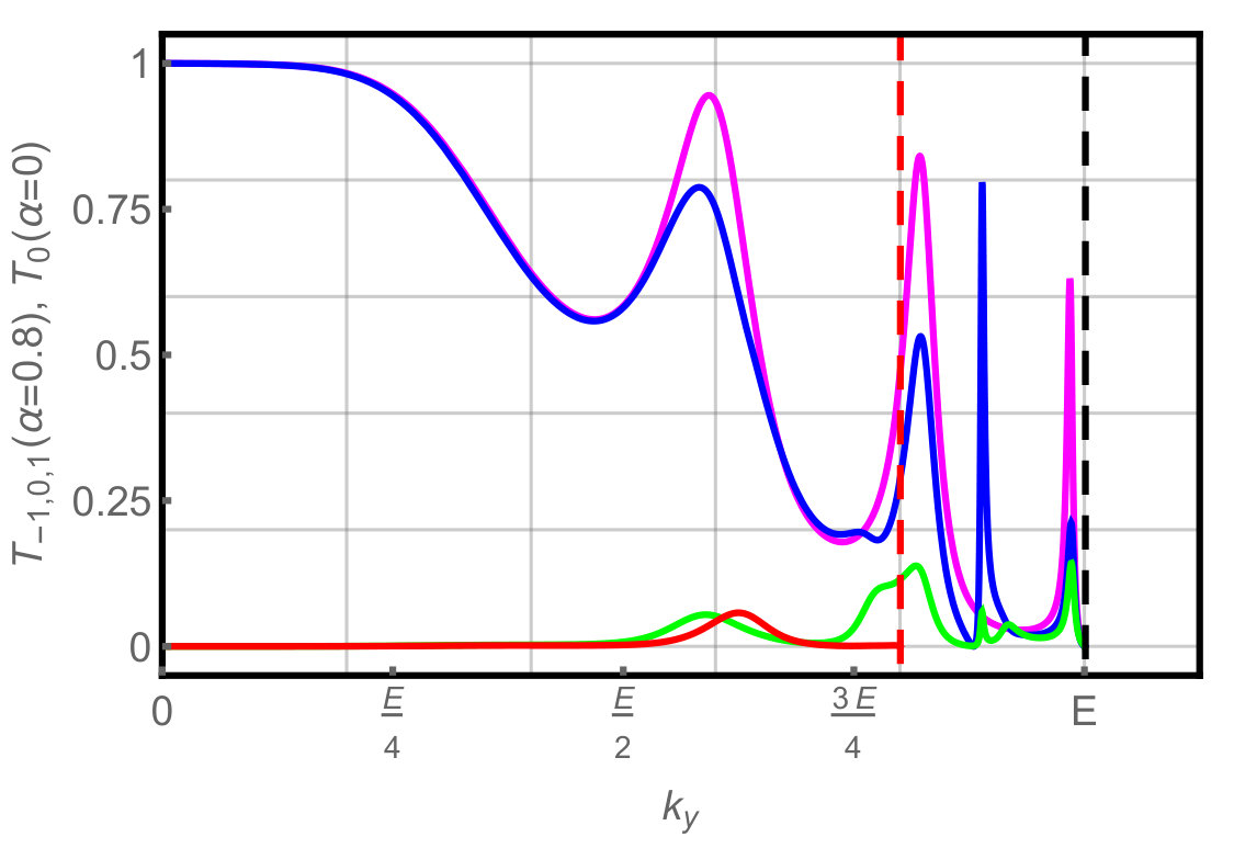 Figure 7
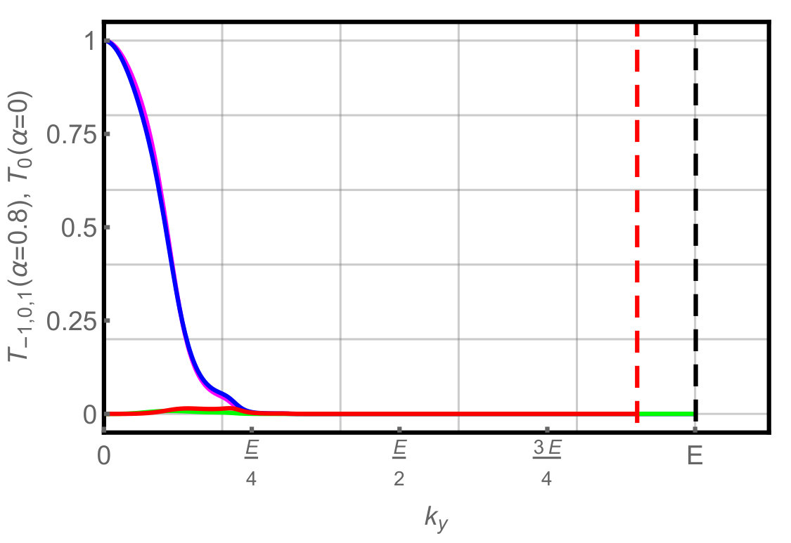 Figure 8
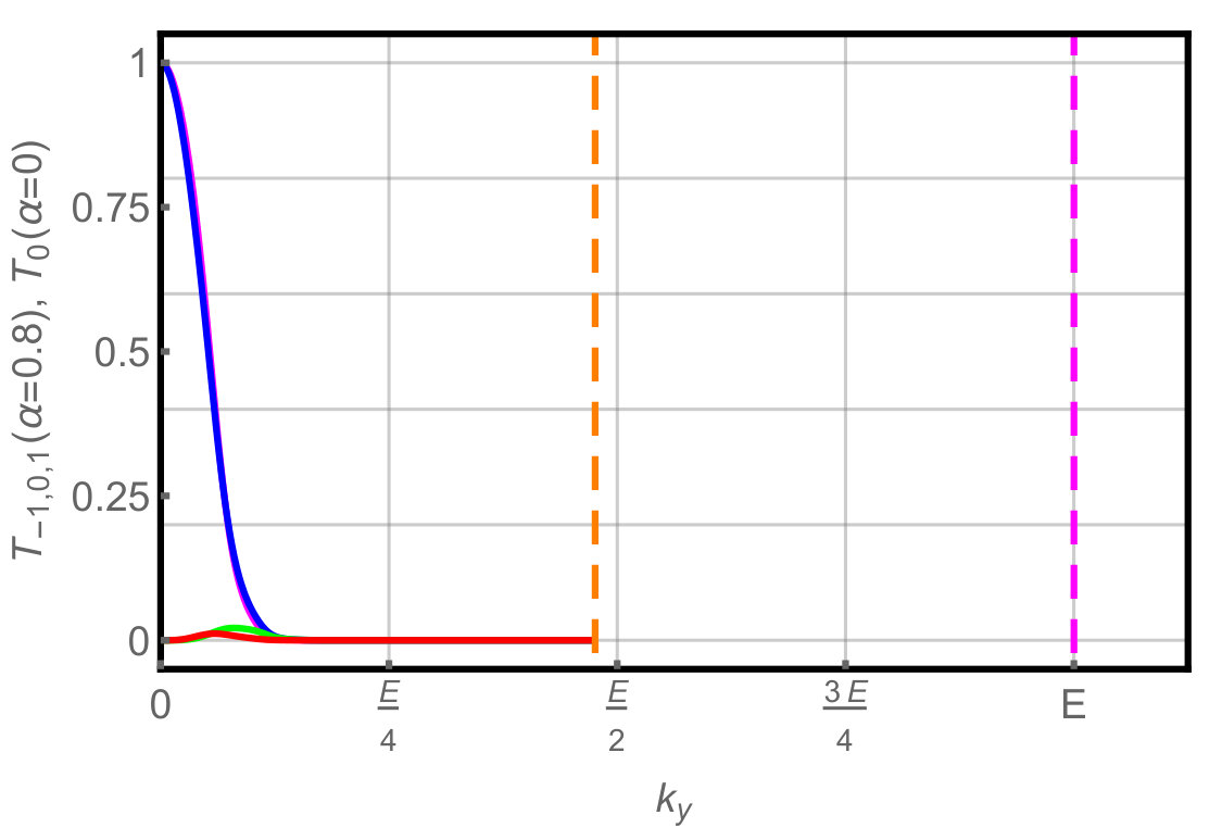 Figure 9
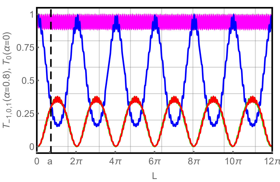 Figure 10
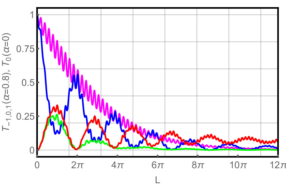 Figure 11
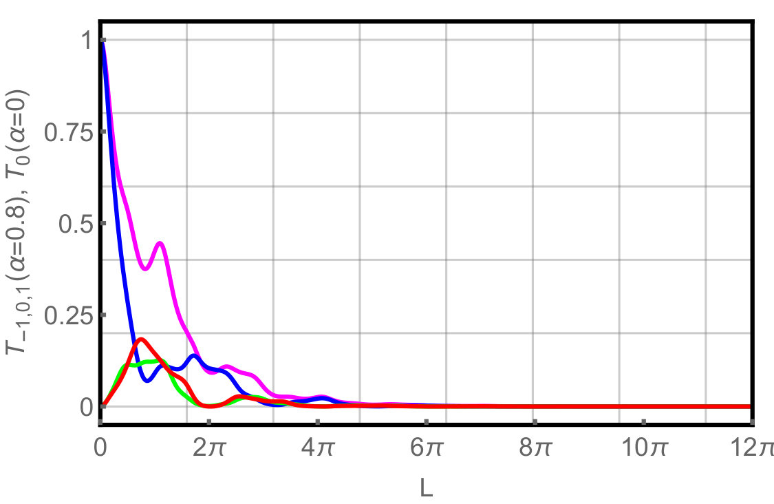 Figure 12
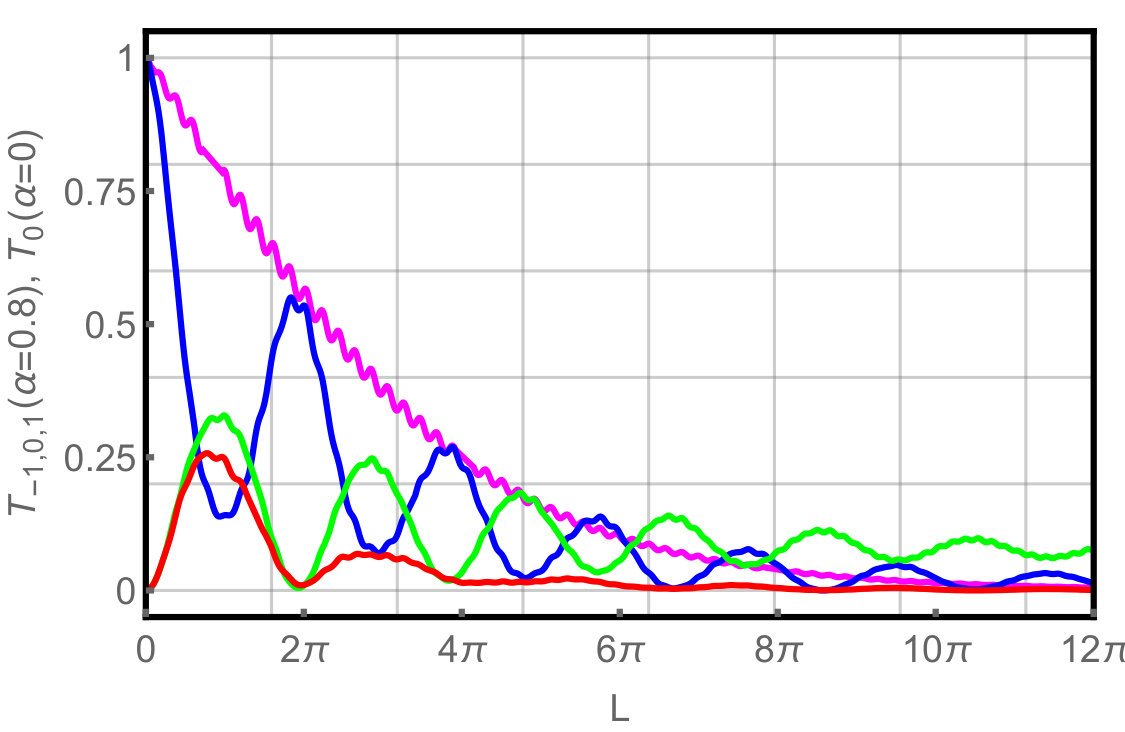 Figure 13
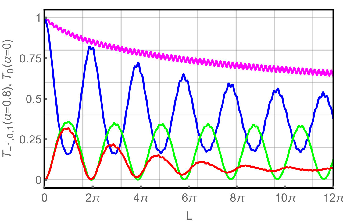 Figure 14
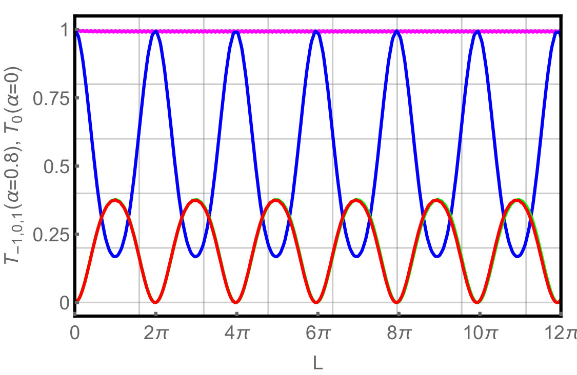 Figure 15
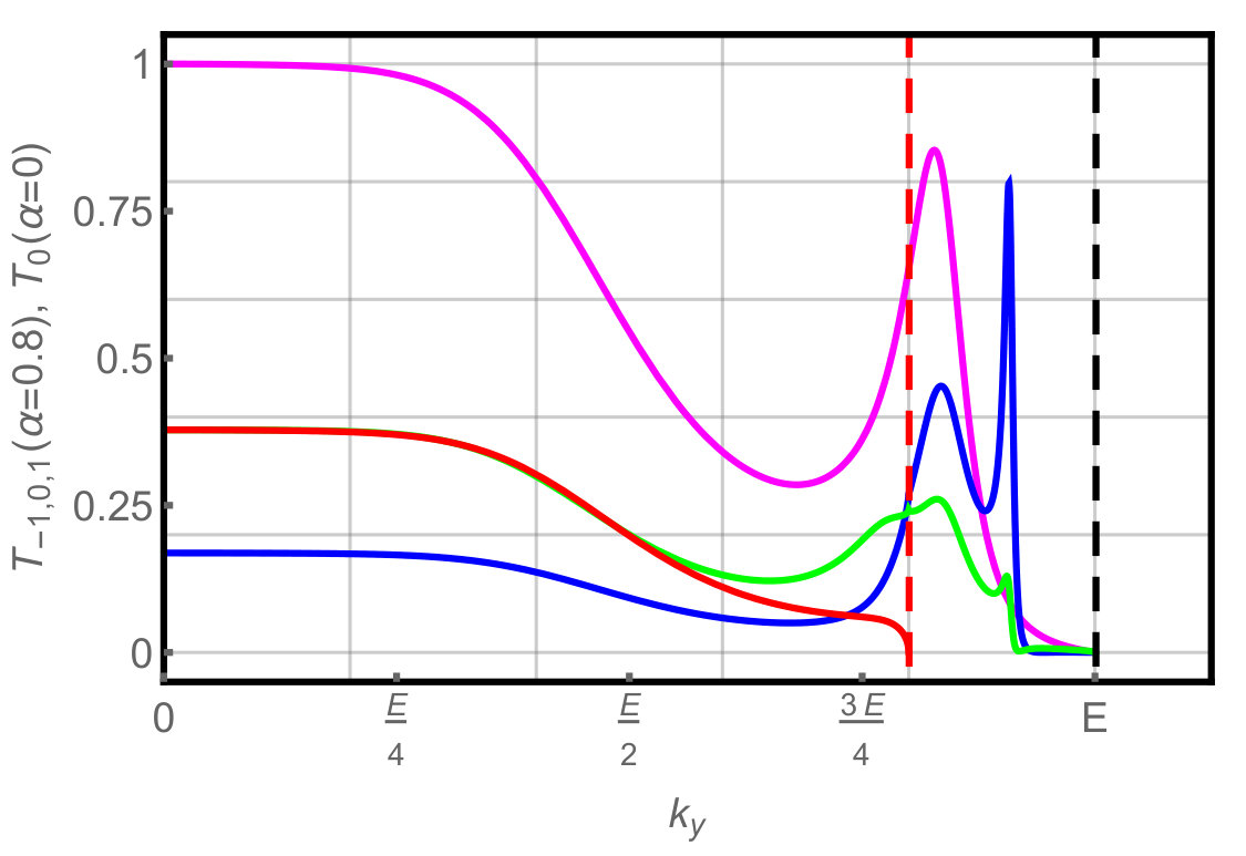 Figure 16
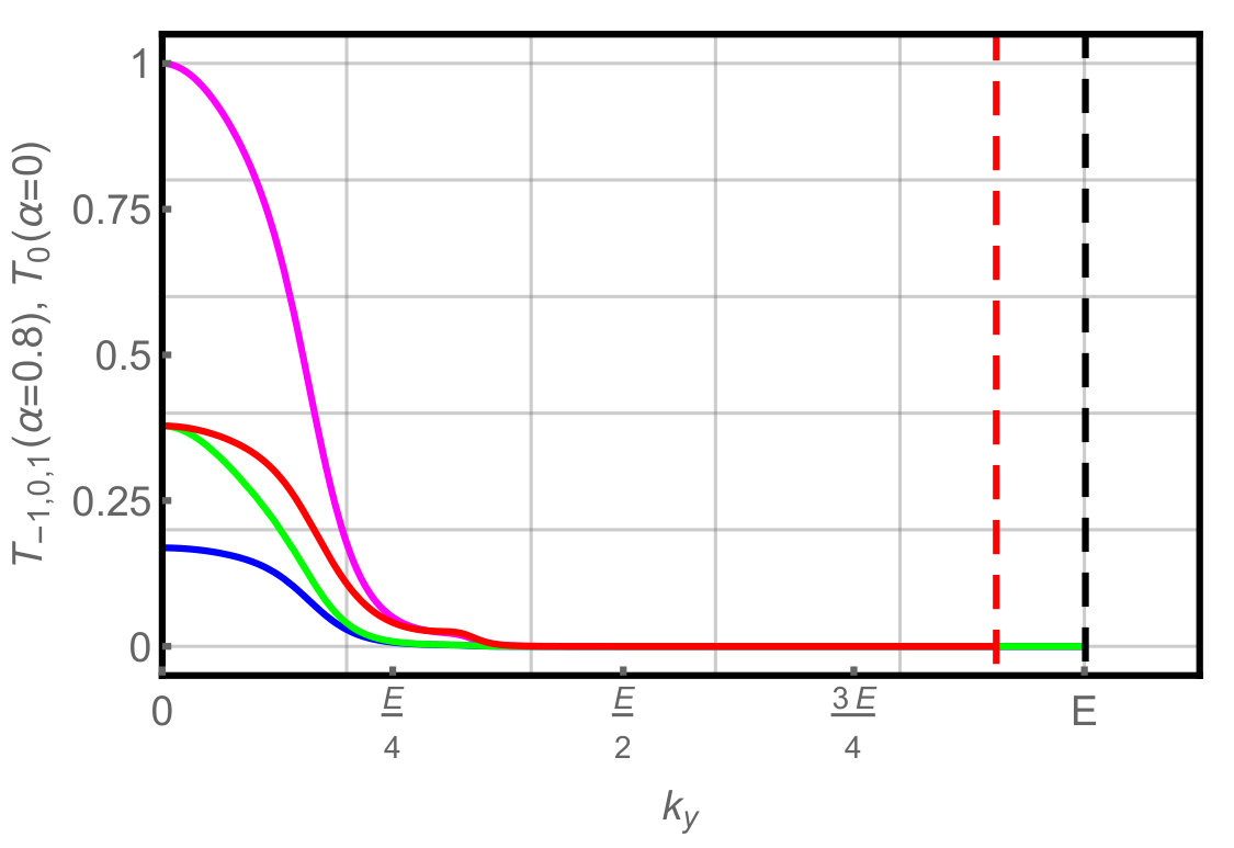 Figure 17
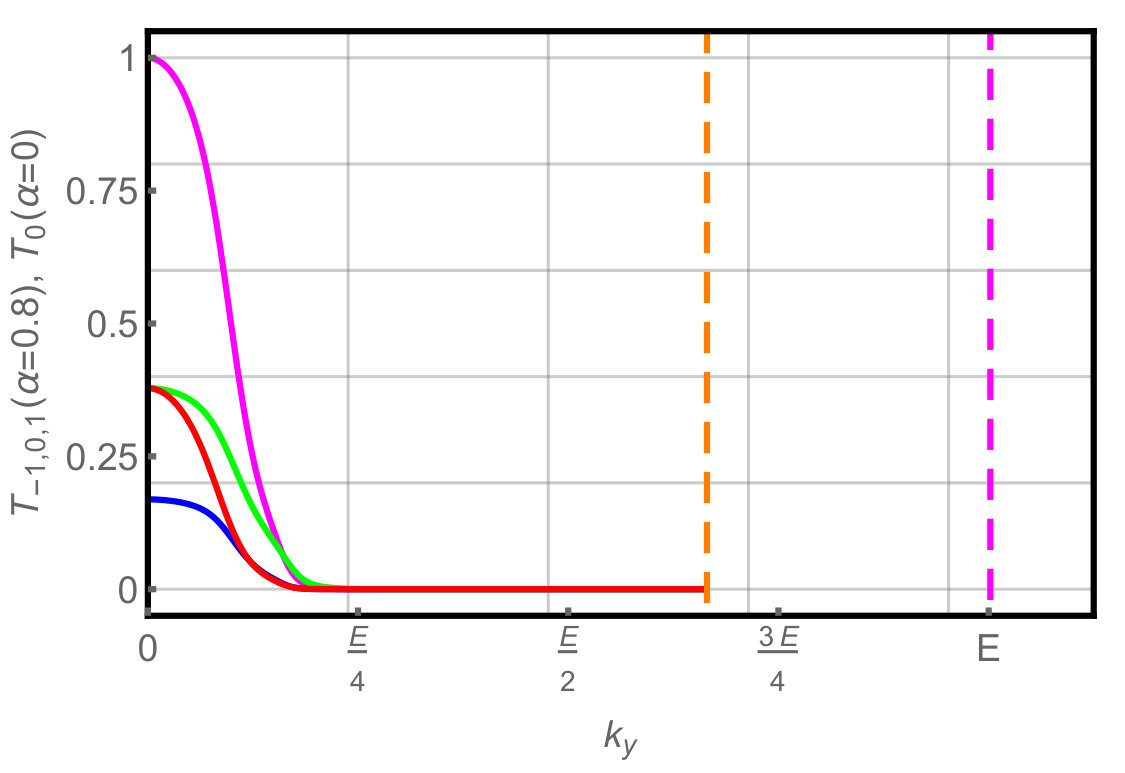 Figure 18
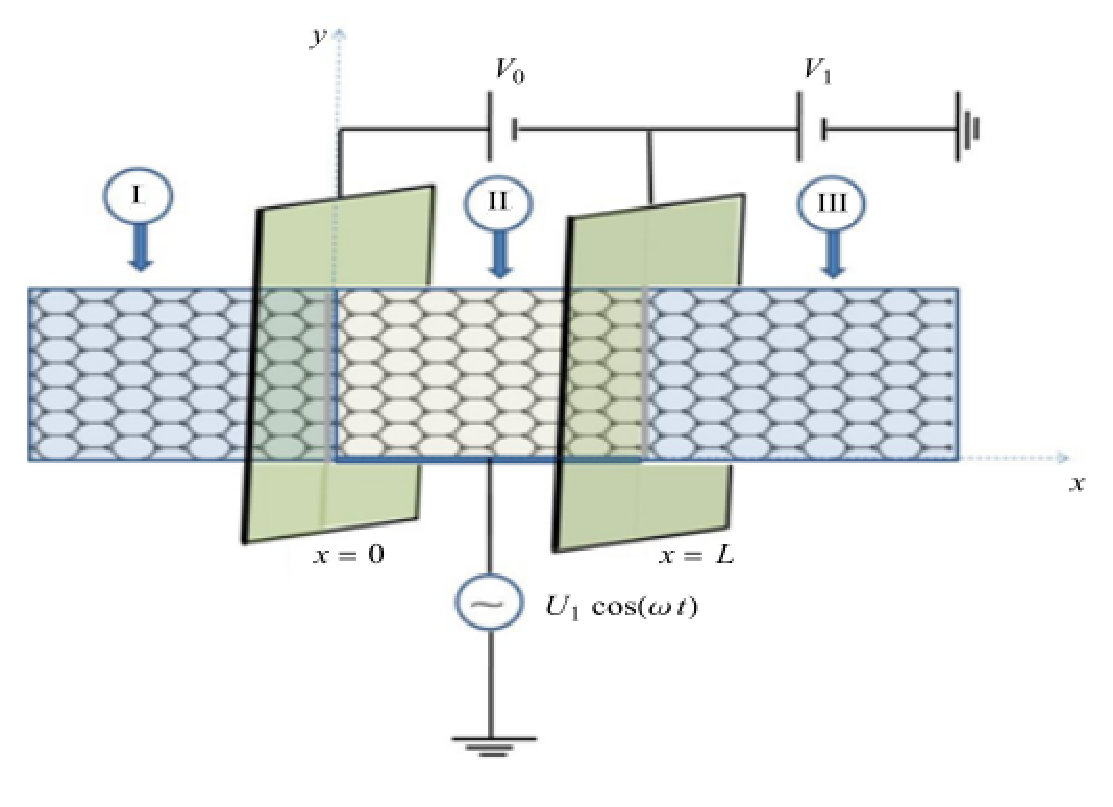 Figure 19
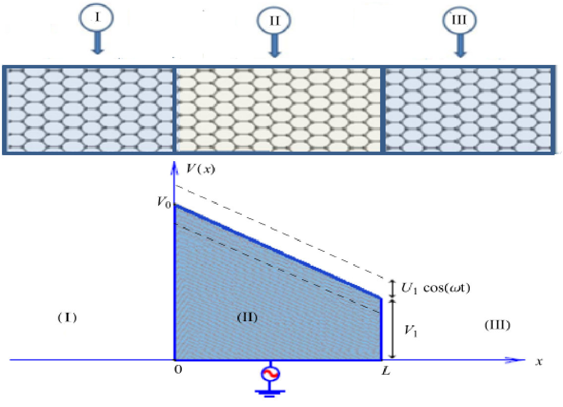 Figure 20
Peer Reviews
No public reviews on file for this paper yet. If you reviewed it on a platform where reviews are public (OpenReview, ICLR, NeurIPS, ICML), you can paste yours below so the community can read it here.
Videos
No videos yet. Explain this paper in a talk, walkthrough, or lecture? Add one.
Taxonomy
TopicsQuantum Information and Cryptography · Quantum optics and atomic interactions · Quantum Mechanics and Applications
Transmission in Graphene through Time-oscillating Linear Barrier
El Bouâzzaoui Choubabi
Laboratory of Theoretical Physics, Faculty of Sciences, Chouaïb Doukkali University,
Ahmed [email protected]
Laboratory of Theoretical Physics, Faculty of Sciences, Chouaïb Doukkali University,
Saudi Center for Theoretical Physics, Dhahran, Saudi Arabia
Miloud Mekkaoui
Laboratory of Theoretical Physics, Faculty of Sciences, Chouaïb Doukkali University,
Transmission probabilities of Dirac fermions in graphene under linear barrier potential oscillating in time are investigated. Solving Dirac equation we end up with the solutions of the energy spectrum depending on several modes coming from the oscillations. These will be used to obtain a transfer matrix that allows to determine transmission amplitudes of all modes. Due to numerical difficulties in truncating the resulting coupled channel equations, we limit ourselves to low quantum channels, i.e. , and study the three corresponding transmission probabilities.
PACS numbers: 72.10.-d; 73.63.-b; 72.80.Rj
Keywords: Graphene, time-oscillating linear potential, Dirac equation, transmission modes.
1 Introduction
Graphene is a stable planar monolayer of densely crystallized carbon atoms in a two-dimensional honeycomb lattice [1]. Since its realization in , graphene has generated an immense interest in studying their mechanical, electronic, optical, thermal and chemical properties [2, 3, 4]. The electronic properties are justified by a relativistic Hamiltonian resulted from Tight-Binding model framework at low energy to the neighborhoods of the six Dirac points at the Brillouin zone corners in the reciprocal lattice. These are represented by two inequivalent points and corresponding to the two atoms and constituting the pattern in the direct lattice. In addition, the fermions in graphene behave as chiral massless particles with a "light speed" equal to the crystal velocity Fermi with a gapless linear dispersion relation near Dirac points. This allows graphene to be a candidate for manufacturing the carbon-based nanoelectronic devices.
Quantum transport in periodically driven quantum systems is an important subject not only of academic value but also for device and optical applications. In particular, quantum interference within an oscillating time-periodic electromagnetic field gives rise to additional sidebands at energies in the transmission probability originating from the fact that electrons exchange energy quanta carried by photons of the oscillating field, being the frequency of the oscillating field. The standard model in this context is that of a time-modulated scalar potential in a finite region of space. It was studied earlier by Dayem and Martin [5] who provided the experimental evidence of photon assisted tunneling in experiments on superconducting films under microwave fields. Later on, Tien and Gordon [6] provided the first theoretical explanation of these experimental observations. Further theoretical studies were performed later by many research groups, in particular Buttiker investigated the barrier traversal time of particles interacting with a time-oscillating barrier [7]. Wagner [8] gave a detailed treatment on photon-assisted tunneling through a strongly driven double barrier tunneling diode. He also studied the transmission probability of electrons traversing a quantum well subject to a harmonic driving force [9] where transmission side-bands have been predicted. Grossmann [10], on the other hand, investigated the tunneling through a double-well perturbed by a monochromatic driving force which gave rise to unexpected modifications in the tunneling phenomenon. Very recently, theoretical studies have suggested that an analog of topological-insulating behavior can be induced in graphene by a time-dependent electric potential [11, 12, 13, 14, 15, 16]. This can be realized by exposing graphene to circularly polarized electromagnetic radiation of wavelength much larger than the physical sample size, such that only the electric field has significant coupling to the electron degrees of freedom [17].
In [18] we have solved the 2D Dirac equation describing graphene in the presence of a linear vector potential. The discretization of the transverse momentum due to the infinite mass boundary condition reduced our 2D Dirac equation to an effective massive 1D Dirac equation with an effective mass equal to the quantized transverse momentum. We have used both a numerical Poincaré map approach, based on space discretization of the original Dirac equation, and a direct analytical method to study tunneling phenomena through a biased graphene strip. It is showed that the numerical results generated by the Poincaré map are in complete agreement with the analytical results. In [19], we have analyzed the energy spectrum of a graphene sheet subject to a magnetic field and a single barrier oscillating in time. The corresponding transmission is studied as function of the incident energy and potential parameters. In particular, it is showed that the time-periodic electrostatic potential generates additional sidebands at energies in the transmission probability originating from the photon absorption or emission within the oscillating barrier.
Based on our previous work [18, 19], we consider a graphene sheet subjected to the oscillating linear barrier potential along the -direction while the carriers are free in the -direction. More precisely, the barrier height of oscillates sinusoidally with the amplitude and frequency . After getting the energy spectrum, we match all wavefunctions to end with a transfer matrix that allow to determine the transmission probabilities for all Floquet side-bands. Since we have many energy modes we focus only on three channels and describe numerically the corresponding transmissions in terms of different physical parameters of our system.
The manuscript is organized as follows. In section 2, we present the theoretical model describing a graphene sheet in the presence of a linear barrier potential oscillating in time. Subsequently, we explicitly determine the eigenvalues and eigenspinors for each region composing our system. The transmission probabilities for all energy modes will be determined using the transfer matrix approach in section 3. In section 4, we numerically present and discuss the transmissions for three channels under suitable conditions of the physical parameters characterizing our system. We conclude our results in the final section.
2 Theoretical formulation
We consider a system composed of three regions (Figure 1) where in regions (I, III) there is only pristine graphene and the intermediate region II is subjected time-harmonic potential of amplitude and driving frequency as well as linear potential generated by the two flat armatures sited at interfaces and . The armatures are identical, with the same surface spaced by a distance , and are perpendicular to the graphene sheet. The condenser (two flat armatures) is biased by a potential difference . We assume that the dimensional requirement allows the condenser to be considered as infinite in order to neglect the edge effects. In the condenser, the electric field prevailing between the two armatures comes from superposition of the electric fields created by each armature, the resultant field remains perpendicular to the armatures. Since such field spatially derives of a potential so the equipotential surfaces are parallel to the armatures and vary gradually linear between the two potentials reported in the armatures. We assume that the graphene sheet passes through grooves at the centers of armatures without disturbing the system (Figure 1) in such a way that the intermediate region of the sheet is subjected to a linear inter-armatures potential (Figure 2) given by
[TABLE]
Note that our system is made of massless Dirac fermions moving along the -direction and being free in the -direction. We assume that the graphene sheet is characterized by very large length scale (-direction) and width (-direction). In input region I, at the interface , the incident fermions of energy and angle with respect to the -direction are reflected with energies and incident angles . In output region III, at the interface , after transmission the fermions have the same energies with transmission angle .
The Hamiltonian system can be written as
[TABLE]
where is the Fermi velocity, are the usual Pauli matrices and is the unit matrix (hereafter we use ). The system has finite width with infinite mass boundary conditions on the wavefunction at boundaries and along the -direction [20, 21]. These result in a quantization of the transverse momentum
[TABLE]
On other hand, the periodic nature of the linear potential necessitates that the solutions of the Dirac fermions are Floquet states. Therefore, we write the eigenspinors as and then from the eigenvalue equation we obtain
[TABLE]
which can be integrated to end up with the solution
[TABLE]
By introducing the expansion in terms of the -th order Bessel function of the first kind , we can write the eigenspinors as
[TABLE]
corresponding to the eigenvalues including the Floquet side-bands
[TABLE]
where we have set . Taking into account of the energy conservation, the eigenspinors that describe the fermions in the -th region can be expressed as a linear combination of those at energies . Thus we have
[TABLE]
and the spinor will be determined by considering each region . Indeed, in region I, solving the time-dependent Dirac equation we can easily get the solution at energy for the incident fermions
[TABLE]
where , is the angle that the incident fermions make with the -direction, and are the and -components of the fermion wave vector, respectively. Because of the oscillation in time of , then the reflected and transmitted waves have components at all energies . Consequently the eigenspinors for reflected fermions are
[TABLE]
and correspond to the eigenvalues
[TABLE]
where is the amplitude of reflection and because the modulation amplitude is in this case. , sign refers to the conduction and valence bands of region I. The number can be obtained from (17)
[TABLE]
Finally combing all to obtain the eigenspinors in region I
[TABLE]
For region II a linear combination of eigenspinors at energies has to be taken and therefore we have
[TABLE]
which can be written in terms of the parabolic cylinder function [18] such that the first component is given by
[TABLE]
corresponding to the energies
[TABLE]
where , , and are constants. The second component takes the form
[TABLE]
The components of the spinor solution of the Dirac equation (2) in region II can be derived from (21) and (23) as
[TABLE]
where we have defined the functions and
[TABLE]
For region III , the eigenspinors for transmitted fermions read as
[TABLE]
where is the amplitude transmission, which can be mapped in terms of the null vector as
[TABLE]
In the forthcoming analysis, we will see how to use the above solutions of the energy spectrum to deal with different issues. In fact, we will employ them to explicitly determine the transmission probabilities for all energy modes.
3 Transmission through oscillating linear barrier
Using the orthogonality of and the continuity of eigenspinors at boundaries (, ), to end up with a set of equations for , , , ,
[TABLE]
Since Dirac fermions pass through a region subjected to time-oscillating linear potential, transitions from the central band to sidebands (channels) at energies occur as fermions ex-change energy quanta with the oscillating field. This procedure is most conveniently expressed in the transfer matrix formalism, such as
[TABLE]
where the total transfer matrix and transfer matrices , that couple the wave function in the -th region to the wave function in the -th region, are
[TABLE]
by setting the quantities
[TABLE]
where the null matrix is denoted by and is the unit matrix. We are considering fermions propagating from left to right with energy , then, , and is the null vector, whereas and are the vectors of transmitted and reflected waves respectively. From the above considerations, one can easily obtain the relation
[TABLE]
The minimum number of sidebands that need to be considered is determined by the strength of the oscillation, . Then the infinite series for can be truncated to consider a finite number of terms starting from up to . Furthermore, analytical results are obtained if we consider small values of and include only the first two sidebands at energies along with the central band at energy . This gives the result
[TABLE]
where and denotes the inverse matrix . Then for , it remains only the transmission for central bands, which gives exactly the result obtained in our previous work [18]
[TABLE]
On the other hand, we can use the reflected and transmitted currents to explicitly determine the transmission and reflection probabilities corresponding to our system. These are defined as
[TABLE]
describes the scattering of fermions with incident energy in the region I into the sideband with energy in region III. Thus, the rank of the transfer matrix increases with the amplitude of the time-oscillating potential. To evaluate (66), we use the Hamiltonian system to show that the current density takes the form
[TABLE]
and now using the solutions of the energy spectrum for each region to end up with the incident, reflected and transmitted currents
[TABLE]
Injecting them into (66) to obtain
[TABLE]
Due to numerical difficulties, we truncate (48) retaining only terms corresponding to the central and first sidebands, namely , which are
[TABLE]
To explore the above results and go deeply in order to underline our system behavior, we will introduce the numerical analysis. For this, we will focus only on few channels and choose different configurations of the physical parameters.
4 Numerical results
In Figure 3, we present the transmission probability versus incident energy . Figure 3LABEL:sub@FigCh01:100 shows the general behavior of the transmission probability of a linear barrier limited by two values of potential (, ) for and , respectively. We observe that the transmission is forbidden below the energy , which behaves like an effective mass [22, 23]. For energies the transmission shows oscillations and gives rise to the Klein paradox, i.e. (Klein zone). In the range of energy , the transmission decreases from until a minimum value where it oscillates and after increases by passing from to reach a maximal value at . However for energy our system shows a classical behavior. To give comparison and show the relevance of our finding, we plots two cases according to choice of the barrier heights . Indeed, Figure 3LABEL:sub@FigCh01:101 illustrates a particular case of a linear barrier (, ) studied in our previous work [18] where transmission corresponding to the Klein zone is omitted and transmission oscillates around a minimum, then it behaves in the same way as shown in 3LABEL:sub@FigCh01:100. Figure 3LABEL:sub@FigCh01:102 presents the case of a simple square barrier where the Klein zone is conserved and transmission corresponding to energies is replaced by another in range without oscillations [24]. Finally, we observe that Figures 3 highlight the effect of the barrier width on transmission, as long as increases the minimal transmission of the intermediate zones decreases and the number of oscillations increases.
In Figures 4 we present the three channel transmissions together with total one (summation over three channels) versus incident energy for , and . These concern the central transmission band (blue color), two first sidebands (red color), (green color), and total (magenta color)
[TABLE]
Since the time-oscillating linear barrier vibrates sinusoidally and longitudinally along the propagating -direction of Dirac fermions, with amplitude and frequency , we notice that this causes a change in the effective mass from to . For low values of the central transmission band is dominant compared to those of lateral 4LABEL:sub@FigCh02:200. As long as increases the central transmission band decreases while the two first sidebands increase. In Figure 4LABEL:sub@FigCh02:201 we have co-dominance of the three bands but in Figure 4LABEL:sub@FigCh02:202 the two first sidebands dominate. We observe that the total transmission decreases if increases. Since is barrier height dependent, the decreasing of might be caused by the missing modes.
Figure 5 shows transmission probabilities and as function of barrier width under suitable conditions. We observe that have a periodicity of except . In Figure 5LABEL:sub@FigCh03:301 and for , transmissions maintain sinusoidal oscillations where are almost equal throughout the periodicity of . Moreover, we notice that for , and , is dominating but for the role changes to and for or are co-dominant. Throughout the variation of , alternately takes values close to unity. Figure 5LABEL:sub@FigCh03:302 presents and for where the transmissions are waning in oscillation as long as increases. For we have the dominance of until . Beyond this value, dominates and the two transmissions are maintained with the increase of , but vanishes at and decays sinusoidally and vanishes at . In Figure 5LABEL:sub@FigCh03:303 and for , we see that all transmission probabilities decay and vanish before . The transmission probabilities in Figure 5LABEL:sub@FigCh03:304 with are similar to those of Figure 5LABEL:sub@FigCh03:302 with , except that the roles of and are inverted. In Figure 5LABEL:sub@FigCh03:305 for all transmissions start to behave in similar way as in Figure 5LABEL:sub@FigCh03:301. In Figure 5LABEL:sub@FigCh03:306 for , and are similar to those seen in Figure 5LABEL:sub@FigCh03:301, the difference is that those of Figure 5LABEL:sub@FigCh03:306 are smooth and thin compared to those in the Figure 5LABEL:sub@FigCh03:301.
Figure 6 shows the transmission probabilities as function of wave vector under suitable conditions. To describe such Figure we divide the interval of into two regions: \Big{\{}R_{1}=]0,k_{y_{1}}[, (with : dashed red line, : dashed black line)\Big{\}} corresponding to Figures (6LABEL:sub@FigCh04:401, 6LABEL:sub@FigCh04:402, 6LABEL:sub@FigCh04:404, 6LABEL:sub@FigCh04:405) and \Big{\{}R_{3}=]0,k_{y_{3}}[, (with : dashed orange line, : dashed magenta line)\Big{\}} corresponding to Figures (6LABEL:sub@FigCh04:403, 6LABEL:sub@FigCh04:406). We observe that for any value of energy, always there is the condition . In and there is manifestation of all transmission modes, but in the mode is missing, and in all modes are forbidden. In (Figure 6LABEL:sub@FigCh04:401), is the first dominant, followed by , which are co-dominant at the beginning and finish by dominance of with respect to . Finally the central band dominates only just before . In (Figure 6LABEL:sub@FigCh04:401), , , show peaks (one peak, two peaks, two peaks) respectively, the first peak of dominates the first peak of that also dominates the first peak of and the second peak of dominates the second peak of . At the beginning of (Figure 6LABEL:sub@FigCh04:404), (, are co-dominant between them and dominate together the two transmissions which are also co-dominant between them. After , each of the four transmissions generates a first peak, where that of is greater than that of , which also greater than that of . The transmissions in (Figure 6LABEL:sub@FigCh04:404) behave in the same way as those in (Figure 6LABEL:sub@FigCh04:401), except towards the end of region one has a generation of a supplementary peak for each transmission with . In (Figure 6LABEL:sub@FigCh04:402), (Figure 6LABEL:sub@FigCh04:403), (Figure 6LABEL:sub@FigCh04:405), and (Figure 6LABEL:sub@FigCh04:406), each transmission probability has one peak. We observe that there are orders: in (Figure 6LABEL:sub@FigCh04:402), in (Figure 6LABEL:sub@FigCh04:403), in (Figure 6LABEL:sub@FigCh04:405) and (Figure 6LABEL:sub@FigCh04:406).
5 Conclusion
We have considered a system composed of three regions of graphene where the intermediate one was subjected to a linear potential barrier oscillating in time with driving frequency along -direction. The infinite mass boundary condition were used to quantize the wave vector along -direction. Due to separability of the eigenspinors we have applied the Floquet theorem to obtain the energy side-bands. By solving the eigenvalue equation, the solutions of the energy spectrum for each region were derived. Moreover, it is showed that the barrier in time generated an infinite modes giving rise to several energy modes.
Subsequently, the transport properties of the present system through transmission probabilities was studied using the transfer matrix approach. Indeed, after matching the eigenspinors at interfaces we have calculated the corresponding transmission and reflections coefficients. There were used together with the current density to explicitly determine the transmission and reflection probabilities as function of the physical parameters. For numerical limitation, we have showed that how the transmission probabilities for the central band () and two first sidebands () are affected by various physical parameters such that incident energy , barrier width and transverse wave vector . These were supported by offering different plots exhibiting the transmission behavior for three side-bands .
In summary, our numerical results support the assertion that quantum interference has an important effect on fermions through graphene based linear barrier driven by time-oscillations. Since most optical applications in electronic devices are based on interference phenomena then we expect that the results of our computations might be of interest to designers of graphene-based electronic devices.
Acknowledgments
The generous support provided by the Saudi Center for Theoretical Physics (SCTP) is highly appreciated by all authors.
Author contribution statement
All authors contributed equally to the paper.
The reference list from the paper itself. Each links out to its DOI / PubMed record.
- 1[1] K. S. Novoselov, A. K. Geim, S. V. Morozov, D. Jiang, Y. Zhang, S. V. Dubonos, I. V. Grigorieva, and A. A. Firsov, Science 306, 666 (2004).
- 2[2] K. S. Novoselov, A. K. Geim, S. V. Morozov, D. Jiang, M. I. Katsnelson, I. V. Grigorieva, S. V. Dubonos, and A. A. Firsov, Nature 438, 197 (2005).
- 3[3] A. H. Castro Neto, F. Guinea, N. M. R. Peres, K. S. Novoselov, and A. K. Geim, Rev. Mod. Phys. 81, 109 (2009).
- 4[4] C. W. Beenakker, Rev. Mod. Phys. 80, 1337 (2008).
- 5[5] A. H. Dayem and R. J. Martin, Phys. Rev. Lett. 8, 246 (1962).
- 6[6] P. K. Tien and J. P. Gordon, Phys. Rev. 129, 647 (1963).
- 7[7] M. Moskalets and M. Buttiker, Phys. Rev. B 66, 035306 (2002).
- 8[8] M. Wagner, Phys. Rev. A 51, 798 (1995).