A bulk-interface correspondence for equatorial waves
Cl\'ement Tauber, Pierre Delplace, Antoine Venaille

TL;DR
This paper demonstrates a topological framework for understanding equatorial waves in fluid dynamics, showing that Kelvin and Yanai waves can be interpreted as topologically protected modes along an interface, with potential applications to coastal waves.
Contribution
It introduces a regularized shallow water model with an odd-viscous term to assign topological invariants to each hemisphere, enabling a bulk-interface correspondence for equatorial waves.
Findings
Kelvin and Yanai waves are shown as exponentially trapped modes along the equator.
The model provides an exactly solvable example of bulk-interface correspondence.
It offers a topological interpretation for transition modes in fluid flows.
Abstract
Topology is bringing new tools for the study of fluid waves. The existence of unidirectional Yanai and Kelvin equatorial waves has been related to a topological invariant, the Chern number, that describes the winding of -plane shallow water eigenmodes around band crossing points in parameter space. In this previous study, the topological invariant was a property of the interface between two hemispheres. Here we ask whether a topological index can be assigned to each hemisphere. We show that this can be done if the shallow water model in -plane geometry is regularized by an additional odd-viscous term. We then compute the spectrum of a shallow water model with a sharp equator separating two flat hemispheres, and recover the Kelvin and Yanai waves as two exponentially trapped waves along the equator, with all the other modes delocalized into the bulk. This model provides an exactly…
Click any figure to enlarge with its caption.
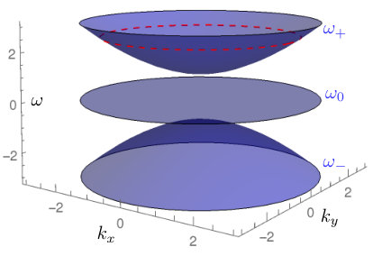 Figure 1
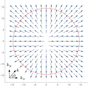 Figure 2
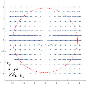 Figure 3
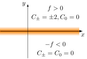 Figure 4
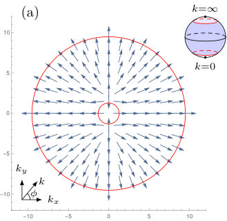 Figure 5
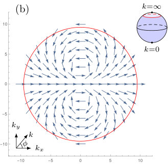 Figure 6
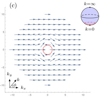 Figure 7
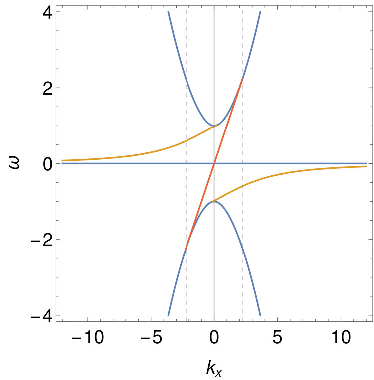 Figure 8
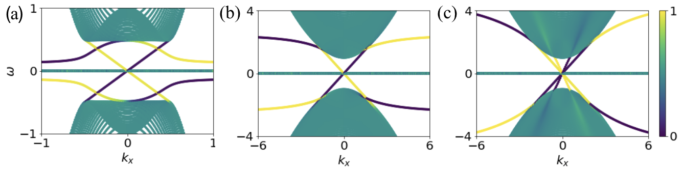 Figure 9
Peer Reviews
No public reviews on file for this paper yet. If you reviewed it on a platform where reviews are public (OpenReview, ICLR, NeurIPS, ICML), you can paste yours below so the community can read it here.
Videos
No videos yet. Explain this paper in a talk, walkthrough, or lecture? Add one.
A bulk-interface correspondence for equatorial waves
C. Tauber\aff1
P. Delplace \aff2
A. Venaille \aff2
\aff1 Institute for Theoretical Physics, ETH Zürich, Wolfgang-Pauli-Str. 27, CH-8093 Zürich, Switzerland \aff2 Univ Lyon, Ens de Lyon, Univ Claude Bernard, CNRS, Laboratoire de Physique, F-69342 Lyon, France
Abstract
Topology is bringing new tools for the study of fluid waves. The existence of unidirectional Yanai and Kelvin equatorial waves has been related to a topological invariant, the Chern number, that describes the winding of -plane shallow water eigenmodes around band crossing points in parameter space. In this previous study, the topological invariant was a property of the interface between two hemispheres. Here we ask whether a topological index can be assigned to each hemisphere. We show that this can be done if the shallow water model in -plane geometry is regularized by an additional odd-viscous term. We then compute the spectrum of a shallow water model with a sharp equator separating two flat hemispheres, and recover the Kelvin and Yanai waves as two exponentially trapped waves along the equator, with all the other modes delocalized into the bulk. This model provides an exactly solvable example of bulk-interface correspondence in a flow with a sharp interface, and offers a topological interpretation for some of the transition modes described by [Iga, Journal of Fluid Mechanics 1995]. It also paves the way towards a topological interpretation of coastal Kelvin waves along a boundary, and more generally, to an understanding of bulk-boundary correspondence in continuous media.
keywords:
Topological Fluid Mechanics, Shallow Water Model, Equatorial Waves, Bulk-boundary correspondence
1 Introduction
Tools from topology developed over the last decades in condensed matter physics have recently shed new light on our understanding of fluid waves, from the design of microfluidic devices (Souslov et al., 2017), to acoustic waves (Yang et al., 2015), to planetary atmospheres (Delplace et al., 2017; Perrot et al., 2018), as well as in active matter flows (Shankar et al., 2017). It has been realized that important and robust information on the spectrum of a linear operator is encoded into the eigenmodes of this operator in unbounded geometry, with constant coefficients. This information is revealed by the winding of the eigenmodes parameterized over a closed surface. This winding is a topological invariant, the Chern number, that can be explicitly computed. For instance, Delplace et al. (2017) showed that inertia-gravity waves in the rotating shallow water model exhibit such a topological property in -space, with the Coriolis parameter, and the wavenumber. More precisely, a Chern number of was found for the positive frequency inertia-gravity waves as they enclose the origin in parameter space, while the zero-frequency (geostrophic) modes carry a vanishing Chern number.
One spectacular manifestation of these singularities occurs when one computes the spectrum of the same operator, now assuming that the one of the parameters varies spatially. In the shallow water model, such computation have for instance been performed by Matsuno (1966) on the equatorial beta plane, assuming linear variations of the Coriolis parameter in the (meridional) direction. He discovered the existence of two branches in the dispersion relation that transit between different wave bands when the wavenumber in the (zonal) direction is varied: the equatorial Kelvin wave, and the mixed Rossby-gravity wave, now known as the Yanai wave. These modes are more localized along the equator than the others, and are unidirectional. The gradient of planetary vorticity also supports the propagation of low frequency planetary Rossby waves, that lift part of the degeneracy of geostrophic modes. However, contrary to the Kelvin and the Yanai waves, the Rossby waves remain in the geostrophic band. Thus, in the equatorial beta plane, when the zonal wavenumber is varied from negative to positive values, the positive frequency inertia-gravity wave band has a net gain of two modes (Delplace et al., 2017). The correspondence between a topological invariant, the first Chern number, that describes degeneracy points for bulk waves in parameter space, on the one hand, and the number of modes that transit from one band to another in the equatorial beta-plane on the other hand, is reminiscent of the Atiyah-Singer index theorem (Faure, 2019; Bal, 2018) and could be referred to as a topological spectral flow correspondence. This correspondence has been proven useful to interpret molecular spectra (Faure & Zhilinskii, 2000), or Lamb-like waves trapped along an interface of density stratification (Perrot et al., 2018), among other applications in physics (Nakahara, 2003).
There exists, however, the possibility for a stronger bulk-interface correspondence, when a topological index can be assigned to each wave band on each side of the interface, rather than to a band-crossing point in parameter space. The bulk-interface correspondence then predicts the number of unidirectional edge states trapped along the interface between the two regions as a consequence of the mismatch between the topological indices of two wavebands across the interface. In condensed matter, thanks to an underlying lattice structure, this bulk-interface correspondence naturally follows from a bulk-boundary correspondence that relates a topological index of the bulk with the number of uni-directional edge modes propagating along a boundary (Hatsugai, 1993; Graf & Porta, 2013). In this context the interface is recovered by gluing together the boundaries of two topologically distinct systems. It is thus natural to ask whether equatorial Kelvin and Yanai waves can also be understood as topological interface states between two distinct topological systems. In other words, can a single hemisphere be interpreted as a topological media on its own? Here we use odd viscous terms to assign a well-defined topological invariant to each hemisphere, building on previous work by Volovik (1988); Souslov et al. (2019), and show that a bulk-interface correspondence is satisfied at the equator.
This example of the linearized rotating shallow water model constitutes an exactly solvable and physically relevant example well suited to clarify ongoing issues related to bulk-interface correspondence in continuous media (Faure, 2019; Bal, 2018), in a case where the interface is sharp. It also offers a novel interpretation of the equatorial waves as two edge states propagating along a sharp equator separating two flat hemispheres that are topologically distinct, with an explicit computation of the spectrum that is complementary to the beta plane case considered by Matsuno (1966), and to the interpretation in terms of transition modes (Iga, 1995), who used arguments based on the conservation of zeros in eigenfunctions.
Finally, this case of a sharp equator for the Coriolis parameter provides a first step towards an understanding of the more complicated case of a sharp boundary for the flow domain, that includes the case of coastal Kelvin waves. In the presence of a boundary, Iga (1995) found that coastal Kelvin waves can be removed from the spectrum just by changing the boundary conditions along the wall. This seems to contradict the expected topological robustness of the boundary modes. It is then natural to ask whether this conclusion is robust to the addition of odd-viscosity (Souslov et al., 2019). We will indeed confirm Iga’s result in that case, which raises an apparent paradox on the applicability of bulk-edge correspondence in fluids.
2 Linearized rotating shallow water equations with odd viscosity
We consider the rotating shallow water equations linearized around a state of rest in Cartesian geometry, with an additional odd viscosity term of amplitude (Avron, 1998)
[TABLE]
where are the two (depth independent) velocity components of the flow in the plane , the interface elevation relative to the mean depth , the Coriolis parameter that may depends on spatial coordinates. The horizontal variations of interface height corresponds to pressure gradients, as the thin layer of fluid satisfies hydrostatic balance. Time unit have been chosen such that the shallow water phase speed is , with the standard gravity.
It was realized two decades ago that a two-dimensional system with broken time reversal symmetry at a microscopic level must include an ’odd viscosity’ term Avron (1998). This term has the same effect on the flow evolution as the Coriolis force, except that its strength depends on the wavenumber. It may be thought of as the first order correction (in ) to the inviscid dynamics that (i) breaks time reversal symmetry (ii) preserves isotropy (iii) does not dissipate energy. The existence of odd-viscous terms is prevented by Onsager reciprocity relations only when the microscopic dynamics is time reversible. This is the case for most classical fluids. However, rotating flows are not time-reversal symmetric. Thus, if subgrid-scales dynamics of a rotating systems are modeled by analogy with molecular effects, an odd viscosity term must be included. Such odd viscosity are actually reminiscent of skew diffusion operators, that have already been proven very useful to model the effect of baroclinic instability in coarse resolution oceans models (Vallis, 2017).
Here, the odd-viscosity term will be essential to assign a topological invariant to the flow model when the Coriolis parameter is prescribed, by regularizing pathological features in bundles of eigenmodes at large wavenumbers. The addition of such terms was also proposed recently by Wiegmann (2013) to describe a fluid of point vortices and by Banerjee et al. (2017); Souslov et al. (2019) for a flow model similar to shallow water equations, motivated by plasma and active matter applications. In the latter work, regularization is also discussed. Moreover this regularization procedure is well-known in a condensed matter context and probably goes back to Volovik (1988) for the Dirac Hamiltonian in two dimensions (see also Bal (2018) for a more general description of this problem). In our case we consider as a (arbitrarily small) constant, and will check that known results are recovered in the the limit . This contrasts with the effect of usual viscosity in three-dimensional turbulence, with the occurrence of anomalous dissipation in the limit of weak viscosity.
Another (complementary) way of removing singularities at large wavenumbers is to consider lattice models, such as the discrete models used for numerical simulations (Delplace et al., 2017). In that case, the admissible wavenumbers are defined on a Torus (called the Brillouin zone in condensed matter), and it is possible to compute the Chern number for the bundle of discretized -plane shallow water eigenmode parameterized on this torus. We leave the study of such discrete models to future work, putting here emphasis on continuous models.
3 Bulk Waves in the f-plane
The bulk problem is defined by the case where the flow takes place in an horizontal unbounded plane with a given . This is the standard -plane approximation. We look at normal modes of the form . The previous system becomes
[TABLE]
where . The band eigenvalues are (see Figure 1 left)
[TABLE]
The middle band is flat, and corresponds to odd-geostrophic modes (pressure terms are balanced by Coriolis and odd-viscous terms). The upper band is an interpolation between two parabolas: when and when , and similarly for the lower one. Those modes correspond to odd-Poincaré (or odd-inertia gravity) waves. Importantly, those bands are separated by a range of forbidden frequencies as long as : the system is gaped. As we shall see it is possible to define a topological invariant, the first Chern number, for each band only in presence of odd-viscosity: .
3.1 Topology of the upper band
Each eigenmode of (4) is defined up to a phase that one can arbitrarily choose locally (gauge freedom), namely for each point of the plane . When such modes are defined onto a closed surface, the existence of a smooth phase everywhere is not guaranteed. In that case, it is always possible to remove a phase singularity at a given point by a suitable gauge choice, but this singularity has to appear somewhere else over the closed surface. The impossibility to define globally a continuous phase is a topological property of the mode, captured by an integer-valued index, the first Chern number. In our case, the difficulty to study these phase singularities originates from the fact that the parameter space is not a closed surface, but the plane . Defining a meaningful topological property for the modes thus requires a compactification of the problem. Even though the compactification of a plane to a (Riemann) sphere is a standard procedure, it is not guaranteed that the eigenmodes defined on the plane can be smoothly mapped on the sphere. In particular, we will show that another kind of singularity of the eigenmodes, appearing at infinity in the plane may prevent the compactification, and thus the definition of the topological property. However, this issue can be overcome thanks to the odd-viscosity term.
At this step, it is judicious to switch to cylindrical coordinates . In particular the bands are -invariant. A normalized (hence non-vanishing) family of eigenvectors associated to is
[TABLE]
up to a phase that can be chosen arbitrarily (gauge freedom). These eigenmodes are regular (single-valued) on the punctured plane . We now ask the following questions: 1) can we extend the regularity property for and ? 2) If yes, can we do it simultaneously? To answer these questions, first notice that
[TABLE]
where is the sign of . is then multivalued, or singular, at 0. But this singularity can be removed using gauge freedom. We define , implying so that is single-valued, or regular on . The problem has been compactified at [math]. Similarly,
[TABLE]
where . The singularity of at can also be cured using gauge freedom. We define , implying so that is regular on the punctured plane where the origin is removed . The problem has been compactified at , in the sense that all the infinite directions are equivalent so that we can consider them as a limiting single point. Importantly, this is not possible without odd-viscosity (). Indeed
[TABLE]
so that the singularity is impossible to remove by the gauge freedom: the problem is not compactifiable at . This is illustrated in Figure 1.
So far the answer to question 1 is positive, but we defined two families and that differ by the choice of a phase, illustrated in Figure 2. The answer to question 2 is captured by the Chern number. The latter is well defined as a topological invariant for compact manifolds only. Here we identify with the two-sphere (see Figure 2), for example through the stereographic projection, although we do not need any explicit transformation. The computation of the topological Chern number is now very standard through the integral of the geometrical Berry curvature (Nakahara, 2003). The Berry curvature is the curl of a Berry connection, that allows one to compare two adjacent normalized eigenmodes in parameter space. For the Berry connection is and the Berry curvature is , independent of . The connection depends on the phase of the eigenmodes, but the curvature is gauge independent.
On one has and thus . The Chern number is the flux of the Berry curvature through the whole (compactified) plane, namely
[TABLE]
Splitting , respectively the disk an its complementary, we apply Stokes theorem on each part and are left with a contribution at the border . Explicitly
[TABLE]
Souslov et al. (2019) reached a similar conclusion for the bulk topology when computing the integral of the Berry curvature over the whole plane , and this result can be recovered for the Dirac Hamiltonian in arbitrary dimension Bal (2018). Note that if we start with the latter derivation leads to , but this is not a Chern number anymore, even if the Berry curvature integrated on the non-compact manifold is finite.
3.2 Topology of the lower and middle bands
The Chern number of the lower band is by the symmetry of the system , leading immediately to . Finally the normalized family of eigenvectors associated to is
[TABLE]
In particular and so that is regular on the whole compactified plane : it is a global continuous section on a compact manifold. Thus . Again, notice that when one has so that the problem is not compactifiable at .
3.3 Summarizing
If and have the same sign , then the Chern number for the three wave bands are and . If and have opposite sign, then . We now compute the wave spectrum when two hemispheres are glued together, with a given value of odd viscosity . According to the bulk-interface correspondence, and whatever the sign of , we expect that 2 unidirectional edge states should fill each frequency gaps between the flat band of geostrophic modes and the inertia-gravity wave bands.
4 Interface: an equator between two flat hemispheres
We consider a sharp interface at between two hemispheres that can now be interpreted as two distinct topological phases (see Figure 3(left)). On the upper half-plane is constant and positive, on the lower one . The parameter is constant and positive on the whole plane. To simplify the computations below we assume .
The translation invariance is preserved in the longitudinal direction, we look for normal modes , the latter vector being a function of variable and parameters and . Dropping the tilde, it is ruled by
[TABLE]
There is a redundancy in the system as is completely determined by and from (13). This can be eliminated, leading to a two dimensional problem of order two:
[TABLE]
At the interface we impose the continuity of and as well as their first derivative
[TABLE]
which implies the same for . We look for the solutions that are localized near the interface, in the sense that they vanish away from it, when . We first solve the problem in each half-plane by decomposing
[TABLE]
and similarly for , then glue the solutions at the interface through (18) and count the remaining degrees of freedom, leading to a number of interface modes. This number is algebraic, its sign being determined by . The result is given in Figure 3 with modes in each gap. We now explain how to reconstruct it.
4.1 The compactified Kelvin wave
It is easy to see that in the whole plane implies . In this section we only assume and look for non-trivial . By (16) we infer , and is ruled by (17), a homogeneous equation of order 2. The solution depends on the relative sign of and .
Case 1: . On the upper half-plane the solution is of the form
[TABLE]
that is always well defined as long as . Notice that (as well as and ) depends on and . For to vanish at we have either or . Here for all and only for , so that
[TABLE]
In the lower half-plane, one has similarly
[TABLE]
but this time we select the positive roots, so that vanishes when . Here and for all so that . From the interface condition (18) we infer two relations between , and for whereas for . More precisely
[TABLE]
We are left with one degree of freedom , a positive dispersion relation that is moreover compactified: the solution exists only for . Note that as . Moreover, in that limit , and . For , so that (23) becomes, after renormalizing ,
[TABLE]
It is remarkable that the limit coincides with the classical (non-compactified) Kelvin wave solution obtained when , in which case the order of the partial differential equation is lowered.
Case 2: . In that case have the same expression but their sign change. A similar inspection leads to for and vanishes otherwise, and for . The gluing condition implies , so that .
4.2 The compactified Yanai wave
In this section we assume and . In that case is entirely fixed by through equation (16), and one can moreover combine (16) and (17) to get a fourth order homogeneous equation for . In the upper half-plane it reads
[TABLE]
The corresponding algebraic equation always admits real solutions as long as , given by with
[TABLE]
In order to get a non trivial mode at the interface, we need both and . This implies
[TABLE]
In the region where oscillatory solutions exist: they are the normal modes from the bulk which are still allowed in the interface setting. This region corresponds to the projection of the bulk bands from (5) for all values of . Thus (27) delimits the gaped region in the interface setting. In this region one has four real solution to (25)
[TABLE]
and similarly for , , where we replace by in the expression of (26). By construction and regardless of or . Consequently,
[TABLE]
Moreover and where
[TABLE]
inferred from (16). The four free parameters and are constrained by the four gluing conditions (18), so that a non-trivial solution exists only if where
[TABLE]
There is no simple expression for the dispersion relation such that , however the latter gives an implicit relation between and , namely
[TABLE]
that can be computed numerically. This way we obtain the Yanai wave of Figure 3: one in each gap. An expansion around shows the behavior , so that the dispersion relation connects (asymptotically) the middle band to the upper band at . On the other hand for a finite value of , an expansion around leads to : the compactified Yanai waves is an inertial wave in this limit, as in Iga (1995) where . For this mode the rank of is 3 so that we only have one free parameter among and : we have Yanai mode in each gap.
The last case with is rather tedious, but it can be checked that no extra mode appear in this case. This is done in supplementary material.
5 Bulk-boundary correspondence and boundary conditions
To emphasize the relevance of the interface studied above we briefly discuss the sharp boundary problem. Figure 4 shows the spectrum of odd-shallow water waves computed numerically with Dedalus (2016) on a channel (or infinite strip) with sharp walls: , where and have the same sign. The boundary conditions are either: , (no slip) or , (stress-free).
Like for the interface, we recover the region of the (projected) bulk bands as well as edge modes in the gaped region, this time localized on each wall. In the following we focus on one of them (e.g ). In Figure 4(a) the number of modes crossing a fixed frequency line in the gap is 2, in agreement with the Chern number of the upper band (Souslov et al., 2019). However this number becomes 1 either when is too close to the middle band or when is smaller: in that case the other mode never crosses the spectral gap windows (Figure 4(b)). Moreover, when changing the boundary condition, the total number of modes surprisingly jumps from 2 to 3 in Figure 4(c).
Thus it seems that the bulk-edge correspondence is not always satisfied for the sharp boundary problem since the number of edge modes depends on the choice of parameters and boundary conditions. On the other hand our interface setting with a canonical choice of gluing condition provides a remarkable case where the bulk-interface correspondence is fully satisfied: the number of modes localized at the interface inside the spectral region matches with the Chern number of the upper band.
6 Discussion and Conclusion
The most representative difference of our study with the original description of equatorial waves by Matsuno (1966) is that we consider a profile with a sharp gap at the equator and constant in each hemisphere, rather than linear variations of the Coriolis parameter with latitude (). In this celebrated equatorial beta plane configuration, all the modes are trapped along the equator, and described by Hermite functions (Matsuno, 1966). Here, in the case of a sharp interface, only the Yanai-like and Kelvin-like waves are exponentially trapped modes; the other modes are all delocalized. In addition, there is no Rossby wave. These properties are caused by the hypothesis of a constant value of in each hemisphere. If we keep the hypothesis of a sharp equator but add back a constant gradient of Coriolis parameter into the problem, topological properties are preserved, but (i) the degeneracy of geostrophic modes is lifted, with the emergence of Rossby waves (ii) all the modes are localized at the equator (like for Hermite functions), even if the Kelvin and Yanai waves remain more localized than the others, which can be understood by counting the zeros of eigenfunctions (Iga, 1995). Using arguments based on the conservation of these zeros, (Iga, 1995) explained the global shape of equatorial wave spectra computed by Matsuno. In particular, he found that the Yanai wave can be interpreted as an inertial wave. Our study brings a complementary point view, showing the topological origin of these properties, as the outcome of gluing two hemispheres with different topological indices. Our analysis also suggests that Yanai waves should be qualified as mixed geostrophic-gravity waves rather than mixed Rossby-gravity waves, as they exist even in the absence of Rossby waves. This result relied on the introduction of a regularization parameter, but we recover the spectrum of the original problem when the regularization coefficient tends to zero: there is no singular limit in the sharp interface case.
To summarize, (i) it has been possible to assign a topological index to each hemisphere through the introduction of odd-viscous term, as in Souslov et al. (2019). (ii) (Souslov et al., 2019) showed a range of parameters and boundary conditions for which the correspondence between the number of unidirectional edge states filling the frequency gap and the bulk Chern number were satisfied. Building on previous work by Iga (1995), we noticed that the number of edge states that transit from one band to another in fact depends on the choice of the boundary condition, even in the presence of odd-viscosity. This new observation raises the question of the existence of a bulk-boundary correspondence for fluids in particular, and for continuous media in general. (iii) We have considered the simpler case of a sharp interface separating the two hemispheres. This interface case bypasses the need to discuss boundary conditions, as the natural physical choice is to impose continuity of the fields and their derivatives. We have found in that case explicit analytical solutions exhibiting exactly two unidirectional modes in each gap confined along the equator, accordingly with the bulk-interface correspondence. Remarkably, this simple case provides a solvable example of a bulk-interface correspondence in fluids, in a configuration where the interface in infinitely sharp. This paves the way towards an understanding of the bulk-edge correspondence in continuous media with boundaries. We will explain in a companion paper that the apparent paradox between the number of edge states and the bulk Chern number can indeed be explained, beyond the particular case of the shallow water model.
Acknowledgements.
C. T. is grateful to Gian Michele Graf and Hansueli Jud for many insightful discussions. P. D. and A.V. were partly funded by ANR-18-CE30-0002-01 during this work, and thank L.-A. Couston for help with Dedalus.
Supplementary material: checking the possible remaining modes at the interface
The last case to study is and , equations (16) and (17) become
[TABLE]
from which we infer
[TABLE]
where
[TABLE]
with the last sign on the right hand side refers to . The roots are the one from (20) and (22) and furthermore
[TABLE]
where refers to .
Case 1: . One has for all and for , so that for and vanishes otherwise. On the lower half-plane and for all so that . The gluing condition (18) implies so that , which is forbidden by assumption (equivalently we are back to the Kelvin solution). There is no extra interface mode in that case.
Case 2: . One has for all and for whereas and for all , so that
[TABLE]
with for . Similarly
[TABLE]
with for since in that case, see (20). For the gluing condition (18) implies so that which is forbidden by assumption. For the four free parameter and are constrained by the four gluing conditions (18). There exist a non-trivial solution only if with
[TABLE]
One can check numerically that along this occurs only twice, and exactly at the crossing with the Yanai wave dispersion relation. This ensures the continuity of the latter and confirms that there is no other mode in that case.
The reference list from the paper itself. Each links out to its DOI / PubMed record.
- 1Avron (1998) Avron, J.E. 1998 Odd viscosity. Journal of statistical physics 92 (3-4), 543–557.
- 2Bal (2018) Bal, G. 2018 Continuous bulk and interface description of topological insulators. ar Xiv preprint ar Xiv:1808.07908 .
- 3Banerjee et al. (2017) Banerjee, D., Souslov, A., Abanov, A. G & Vitelli, V. 2017 Odd viscosity in chiral active fluids. Nature Communications 8 (1), 1573.
- 4Dedalus (2016) Dedalus, Project 2016 http://ascl.net/1603.015 , http://dedalus-project.org .
- 5Delplace et al. (2017) Delplace, P., Marston, J.B. & Venaille, A. 2017 Topological origin of equatorial waves. Science p. eaan 8819.
- 6Faure (2019) Faure, F. 2019 Manifestation of the topological index formula in quantum waves and geophysical waves. https://arxiv.org/abs/1901.10592 .
- 7Faure & Zhilinskii (2000) Faure, F. & Zhilinskii, B. 2000 Topological Chern indices in molecular spectra. Physical review letters 85 (5), 960.
- 8Graf & Porta (2013) Graf, G. M. & Porta, M. 2013 Bulk-edge correspondence for two-dimensional topological insulators. Communications in Mathematical Physics 324 (3), 851–895.